Enhancing Waste-to-Energy and Hydrogen Production through Urban–Industrial Symbiosis: A Multi-Objective Optimisation Model Incorporating a Bayesian Best-Worst Method

Abstract

A surging demand for sustainable energy and the urgency to lower greenhouse gas emissions is driving industrial systems towards more eco-friendly and cost-effective models. Biogas from agricultural and municipal organic waste is gaining momentum as a renewable energy source. Concurrently, the European Hydrogen Strategy focuses on green hydrogen for decarbonising the industrial and transportation sectors. This paper presents a multi-objective network design model for urban–industrial symbiosis, incorporating anaerobic digestion, cogeneration, photovoltaic, and hydrogen production technologies. Additionally, a Bayesian best-worst method is used to evaluate the weights of the sustainability aspects by decision-makers, integrating these into the mathematical model. The model optimises industrial plant locations considering economic, environmental, and social parameters, including the net present value, energy consumption, and carbon footprint. The model’s functionalities are demonstrated through a real-world case study based in Emilia Romagna, Italy. It is subject to sensitivity analysis to evaluate how changes in the inputs affect the outcomes and highlights feasible trade-offs through the exploration of the $ϵ$-constraint. The findings demonstrate that the model substantially boosts energy and hydrogen production. It is not only economically viable but also reduces the carbon footprint associated with fossil fuels and landfilling. Additionally, it contributes to job creation. This research has significant implications, with potential future studies intended to focus on system resilience, plant location optimisation, and sustainability assessment.

1. Introduction

In 2019, global atmospheric emissions were approximately 59 ± 6.6 GtCO₂eq, marking a significant surge in CO₂ levels to 410 parts per million, a peak not witnessed since pre-industrial times [1]. This alarming increase underscores the urgent necessity for climate change countermeasures, particularly through renewable energy adoption, as highlighted in the European Renewable Energy Directive (RED 2018/2001/EU), which sets an ambitious target of at least 42.5% renewable energy by 2030. The European Green Deal further advocates for the escalated use of recycled materials in industrial sectors to nurture a green, sustainable economy, and to enhance cleaner and more efficient transport systems, which are responsible for a quarter of emissions.

Currently, urban areas are estimated to account for about half of the world’s waste production and roughly 80% of GHG emissions. Each year, approximately 740 Mt of municipal solid waste (MSW) is disposed of in landfills, representing 37% of the global MSW total. Utilising waste management techniques can significantly reduce waste volume, lower pollutant generation, and decrease the spatial footprint needed for waste processing facilities compared to landfills. Additionally, employing anaerobic digesters (ADs) not only contributes to managing waste but also produces digestate, a valuable by-product that can be used as an agricultural fertiliser [2]. The Emilia-Romagna region in northern Italy, known for its rich agricultural background and robust industrial sector, produced 2,839,452 tonnes of urban waste in 2021. The most commonly collected materials were organic and green waste (19% and 6% potentially recoverable). The region also generated 451,423 tonnes of waste from agriculture and forestry, with 99,894 tonnes earmarked for disposal [3]. Waste-to-energy (WtE) technologies are being examined for their potential to effectively recover energy from waste materials [4]. Among these, anaerobic digestion stands out as a WtE technology offering numerous benefits for solid waste management and agriculture. Anaerobic digestion generates biogas, which can be utilised to produce renewable energy while simultaneously reducing waste volume. Biogas can be employed for heat and power generation [5], thereby diminishing reliance on fossil fuels and fostering a more economical and sustainable energy supply [6]. Furthermore, ADs yield a nutrient-rich digestate, serving as a natural fertiliser to improve soil quality and crop yields, reducing dependency on chemical fertilisers [7].

A particular focus in Emilia-Romagna is the development of green hydrogen for both mobility and energy production. The primary challenge in this endeavour lies in the economic viability, given the substantial initial and operational costs. A gradual transition is envisioned, starting with the integration of hydrogen into existing natural gas infrastructures, moving towards electrolysis powered by renewable electricity sources, particularly for heavy transport and industries that are difficult to decarbonise. Effective management of municipal and rural waste, along with establishing a proficient hydrogen supply chain, are, therefore, pivotal areas of interest for stakeholders in the region. Hydrogen is a versatile medium for energy storage, transportation, and electricity production. Currently, the majority of the world’s hydrogen is produced from natural gas and coal [8], with renewables contributing a mere 2% to the total output [9]. The transition to a sustainable energy system by 2050 necessitates a shift towards low-carbon hydrogen [10]. The power-to-hydrogen process converts extra electricity into hydrogen using electrolysis, breaking water molecules into O₂ and H₂. When this electricity is derived from renewable sources, the resultant hydrogen, termed “green hydrogen”, has a substantially lower global warming potential compared to conventional coal gasification and reforming methods [11]. The biomass–electricity–electrolysis pathway is, thus, seen as having superior environmental benefits [12,13]. Green hydrogen also has the potential to drive low-carbon mobility, fostering synergies between industrial sectors and communities [14].

Industrial symbiosis (IS) focuses on resource exchange between companies and has evolved over time. Originally defined over two decades ago within the broader concept of industrial ecology (IE), recent interpretations incorporate modern industrial aspects like mutual learning and life-cycle analysis [15,16]. The process of establishing IS is divided into three phases: exploration of potential collaborations, a critical phase of organisation and development, and finally, the realisation of symbiosis through investments in exchange facilities [17,18]. This approach not only fosters new business opportunities but also enhances supply chain resilience by increasing network connectivity and exchange density, thereby optimising waste management and adding value to waste exchanges [19]. The urban–industrial symbiosis (UIS) concept, as an innovative strategy, promotes sustainable development and efficient resource utilisation across industrial, urban, and rural areas [20]. This approach, facilitated by geographical proximity, enhances trust and reduces logistical challenges, leading to decreased resource consumption, waste, and greenhouse gas emissions, and achieving economic and environmental benefits [21].

The model proposes the creation of an energy-based UIS system that converts biomass into biogas, heat, electricity, and hydrogen through electrolysis. The model aims to assist in planning the use of by-products, particularly fertilisers produced during the anaerobic digestion process, to optimise the economic and environmental impacts of the entire system, with a particular emphasis on the development of a hydrogen supply chain.

This paper includes a concise literature review in Section 2, problem description and formulation in Section 3, a detailed case study in Section 4, followed by results and a sensitivity analysis in Section 5, trade-offs analysis and discussion in Section 6, and provides concluding remarks in Section 7.

2. Literature Review

In recent years, WtE methodologies have become increasingly important for waste management and sustainable energy production. A key tool in this field is mixed integer linear programming (MILP), known for its flexibility in integrating various decision factors and parameters. MILP models are primarily used for designing waste supply chain networks, focusing on waste allocation, and optimising the number, capacities, and locations of waste treatment plants to balance economic, environmental, and social impacts.

Several studies have made notable contributions using MILP, as presented in

Table 1. Summary of the literature of waste-to-energy supply chain networks.

Reference	Source					Output					Objective (s)
	MSW	RW	FW	PV	WP	P	H	H2	F	BF	Eco	Env	Soc
Kim et al. [22]			X							X	X
Gondal and Sahir [23]		X						X			X
Balaman and Selim [24]		X				X	X		X		X	X
Patrizio et al. [25]		X				X	X			X	X
Wu et al. [26]		X	X							X	X
Mayerle and de Figueiredo [27]		X				X	X		X		X
Woo et al. [28]		X	X					X			X
López-Díaz et al. [29]		X								X	X
Silva et al. [30]		X								X	X		X
Han and Kim [31]				X	X	X				X
Bijarchiyan et al. [32]		X				X	X		X		X		X
Maha et al. [33]		X		X		X		X			X
Thiriet et al. [34]	X					X	X				X
Rahimi et al. [35]		X				X			X		X
Abbasi et al. [36]	X					X	X				X	X
This Study	X	X		X		X	X	X	X		X	X	X

Notes: MSW: Municipal Solid Waste, RW: Rural Waste, FW: Forestry Waste, PV: Photovoltaic System, WP: Wind Power, P: Power, H: Heat, H2: Hydrogen, F: Fertiliser, BF: Biofuel, Eco: Economic, Env: Environmental, Soc: Social.

. Kim et al. [22] developed a comprehensive optimisation model for selecting and sizing fuel conversion technologies, focusing on biomass source location, processing plant decisions, and logistics to maximise profit. Gondal and Sahir [23] highlighted the potential of Pakistan’s agrarian economy as a significant source of biomass for hydrogen production. The study introduces an integrated renewable hydrogen model that utilises biomass feedstocks, demonstrating its effectiveness in generating hydrogen. Balaman and Selim [24] optimised biomass-to-energy supply chain networks at regional level in Turkey. Their MILP model considered economic and environmental criteria to identify the optimal number, capacities, and locations of biogas plants and biomass storages. Patrizio et al. [25] explored the potential of agricultural biogas in Italy for power generation, heat cogeneration, and biomethane use in transport and grid injection, using the BeWhere model for optimal location and technology mix assessment.

Wu et al. [26] addressed the optimisation of biomethane production systems location and resource allocation. Their study employs a mixed integer nonlinear programming model to minimise supply chain costs, encompassing construction, transportation, and labour. The model integrates elements like local farms, collection hubs, and biomethane reactors. Mayerle and de Figueiredo [27] focused on supply chain network design for anaerobic digestion and energy generation using animal waste. Addressing the high transportation costs of animal biomass, a methodology was developed to optimise logistics and reduce biogas loss. Woo et al. [28] introduces a MILP model aimed at minimising total annual costs by optimising a biomass-to-hydrogen supply chain. This involves biomass inventories, gasification plants, hydrogen storage, and fuelling stations. López-Díaz et al. [29] investigated the impact of bio-refining supply chains on regional water resources. Their optimisation framework considers the entire bio-refining system, including biomass production, processing, fresh water usage, and wastewater discharge, while integrating economic and environmental objectives. The study places special emphasis on the optimal use of water resources and the selection of feedstocks, cultivation sites, and processing facilities.

Silva et al. [30] tackled biogas plant location for animal waste treatment from dairy farms, considering economic and social factors. Their study introduces a multi-objective MILP model that focuses on minimising initial investment, operation, and maintenance costs, transportation costs, and social rejection. Han and Kim [31] offer a comprehensive method for strategic investment in renewable energy systems, integrating wind, solar, and biomass sources. Using MILP, the study focuses on optimal investment timing and allocation for various energy facilities and demands. Bijarchiyan et al. [32] modelled a biomass-to-bioenergy supply chain using ADs maximising economic profits and positive social externalities. Maha et al. [33] developed an optimisation model for a hydrogen supply chain in Johor, using oil palm biomass and solar energy for hydrogen and electricity production.

Thiriet et al. [34] described an approach to design a network of distributed micro-scale ADs for the valorisation of urban bio-waste. Their MILP model aimed to minimise the total payload distances involved in transporting waste and digestate. Rahimi et al. [35] designed an electricity production supply chain from animal manure, minimising supply chain costs. They determined the best locations for establishing facilities, optimal capacity levels, and material flow. In the context of MSW management, Abbasi et al. [36] considered MSW management, comparing anaerobic digestion and incineration processes to minimise environmental impact while maximising profits.

These studies collectively demonstrate the versatility and effectiveness of MILP in optimising WtE systems, balancing economic viability with environmental sustainability. However, there is a growing need for a new, more comprehensive model that intertwines MSW and agricultural biomass waste. This model should ideally incorporate agrivoltaic systems (which couple agriculture and solar power generation) and encompass the production of power, heat, and hydrogen. The development of a multi-objective optimisation model is essential, one that targets not only economic profitability but also strives to establish a low-carbon supply chain. Additionally, this model must take into account social impacts, ensuring that the solutions proposed are not only efficient and sustainable but also socially responsible and acceptable. Such an integrative approach would represent a significant advancement in the field, addressing the multifaceted challenges of modern waste management and energy production. Here are three key points summarising the contribution of this research:

• Creating a novel model that combines MSW and agricultural biomass waste with agrivoltaic systems, addressing multiple aspects of waste and energy management in a unified approach;
• Balancing economic profitability, environmental sustainability (specifically low-carbon supply chains), and social impacts, ensuring a comprehensive and responsible approach to WtE systems;
• Designing a system that simultaneously addresses the production of power, heat, and hydrogen, showcasing a versatile and efficient solution in sustainable energy.

3. Material and Methods

The proposed model is focused on designing a WtE system for organic waste, utilising AD as a key component. In this section, we outline the challenge of creating a WtE system and offer a mathematical representation of the multi-tiered, interconnected biogas–hydrogen network.

3.1. Problem Definition

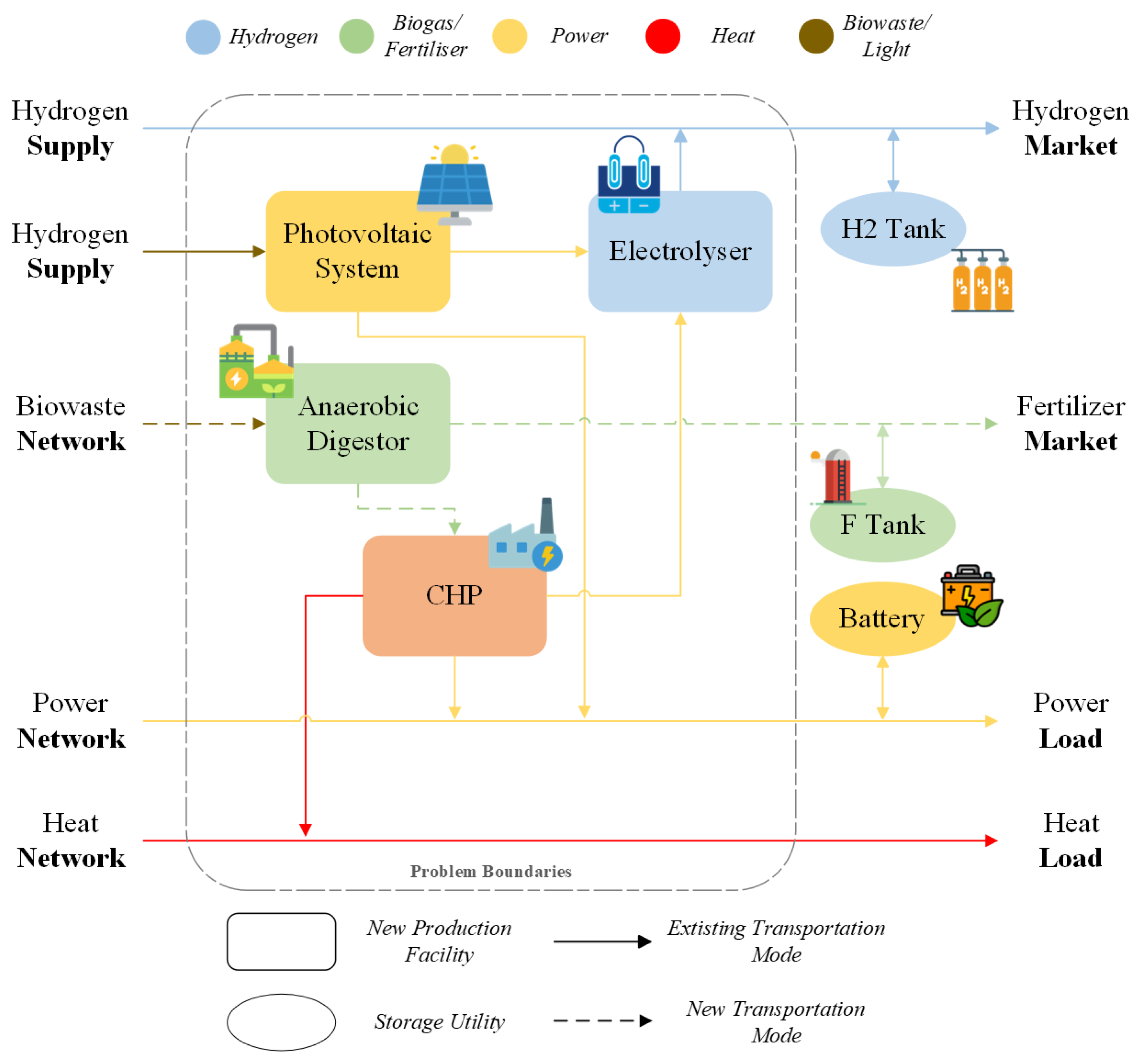
We now turn to the issue of waste-to-energy (WtE) and hydrogen supply chain management. Our proposed model examines a multi-layered network, encompassing nodes for MSW and livestock manure, ADs, solar photovoltaic systems, cogeneration units, electrolysis stations, and relevant storage facilities, as illustrated in Figure 1. The model aims to assist in making strategic decisions regarding the ideal placement of ADs, photovoltaic systems (PVs), combined heat and power plants (CHPPs), and electrolysis units, along with determining their optimal capacities and storage solutions over a set time frame. Furthermore, the model guides decision-makers in managing transportation routes for various materials, including manure, the organic fraction of solid waste, produced biogas, heat, electricity, and hydrogen throughout the network. This is performed with the objective of optimising total costs, reducing GHG emissions, and fostering job creation, thereby adhering to the three pillars of sustainability.

The network begins with the collection of MSW and livestock manure from diverse urban and rural areas. The organic components of this waste are processed in ADs, where they undergo decomposition by microorganisms in an oxygen-free environment. This process yields biogas, a renewable energy source, and digestate, a nutrient-rich fertiliser for agriculture. Concurrently, PVs in selected areas convert sunlight into electricity, which can be used immediately or stored in batteries. The biogas from ADs is utilised in CHPPs, generating electricity and heat. Additionally, electricity from both solar PVs and CHPPs is employed in electrolysis units to produce hydrogen and oxygen from water. This hydrogen, a clean energy source, is stored for future use. The outputs are then stored and distributed as needed, employing a mix of different capacity trucks, along with existing grids and pipelines.

Before running the model, we made several assumptions to ensure its accuracy and relevance to real-world scenarios. These assumptions were chosen based on the level of detail that has been found useful for addressing similar problems in the existing literature.

• Biowaste supply, treated as deterministic across time periods, includes categories like cattle slurry, cattle manure, and the organic/green fraction of municipal wastes.
• Parameters for major facilities encompassing conversion efficiency, capacity, lifetime, investment, and operating costs are given.
• Parameters for hydrogen and fertiliser tanks involving capacity are given.
• Distances between locations are given by regional data.

3.2. Mathematical Model

3.2.1. Objective Functions

Concerns about sustainability are increasingly pushing supply chain managers to make more effective decisions. Human activities have a detrimental effect on natural resources and the environment. The considered approach seeks to mitigate the negative effects of human activities. UIS aims to balance economic benefits through innovative energy business models, reduce emissions from traditional linear economic activities, and generate social benefits by creating jobs. The goal is to assess sustainability from three perspectives: economic, social, and environmental. All relevant sets, parameters, and variables are reported in Appendix A.

The first objective function seeks to maximise the system’s overall economic net present value. This covers the expenses of installing ADs, CHPPs, PVs, and electrolysers, as well as the costs of operating and maintaining them, transporting feedstock and biogas, and producing hydrogen. The revenues are generated from the sale of electricity, heat, hydrogen, and fertiliser produced within the system.

$$\begin{array}{c}\hfill Z_1=-TIC-\sum _{t\in T}\left(AO{C}_t-AT{R}_t\right)\frac{1}{{(1+r)}^t}\end{array}$$

(1)

Equation (2) calculates the total initial cost ($TIC$), which includes the investment costs for installing ADs, CHPPs, electrolysers, and PVs. The cost of each facility type is weighted by its respective capacity and whether it is built or not (indicated by the binary variables).

$$\begin{array}{c}\hfill TIC=\sum _{k\in K}\left(\sum _{a\in A}ic{a}_k^{AD}b{a}_{ak}+\sum _{c\in C}ic{c}_k^{HP}b{c}_{ck}+\sum _{e\in E}ic{e}_k^{EL}b{e}_{ek}+\sum _{p\in P}ic{p}_k^{PV}b{p}_{pk}\right)\end{array}$$

(2)

Equation (3) calculates the annual operating costs ($AOC$), accounting for the operational expenses, transportation costs of feedstock and biogas, and the time value of money. It includes the costs of operating and maintaining the installed facilities and the costs related to transportation, all discounted to their present value.

$$\begin{array}{c}\hfill AO{C}_t=TIC·op+\left(\sum _{f\in F}\sum _{a\in A}\frac{x_{fa}^t}{ca{p}^{TR}}{d}_{fa}+\sum _{a\in A}\sum _{c\in C}\frac{y_{ac}^t}{ca{p}^{TR}}{t}_{ac}\right)·tc\end{array}$$

(3)

The annual total revenue ($ATR$) in Equation (4) calculates the yearly income generated from selling electricity, heat, hydrogen, and fertiliser produced within the system. It considers the quantities of these products sold and their respective unit prices, all discounted to their present value.

$$\begin{array}{cc}\hfill AT{R}_t& =pa\sum _{a\in A}{f}_a^t+pp\sum _{c\in C}\left(e_c^t-\sum _{e\in E}{z}_{ce}^t\right)\hfill \\ & +pp\sum _{p\in P}\left(s_p^t-\sum _{e\in E}{l}_{pe}^t\right)+ph\sum _{c\in C}{q}_c^t+pe\sum _{e\in E}{w}_e^t\hfill \end{array}$$

(4)

The secondary objective $Z_2$ encapsulated within Equation (5) is to minimise the environmental impacts within the supply chain. This goal is pursued through an assessment and minimisation of $\mathrm{C}{\mathrm{O}}_{\mathrm{2}}$ emission factors. Primary focal points include emissions stemming from road transportation linking feedstock sources to AD facilities, and the subsequent transit between AD and CHPP nodes $\left(ETF\right)$. Additionally, it incorporates emissions attributable to the operational processes within these production units $\left(EBE\right)$. $Z_2$ quantifies the environmental advantages derived from diminished natural gas usage (primary non-renewable energy carrier) and the application of fertilisers generated as by-products among the network.

$$\begin{array}{c}\hfill Z_2=ETF+EBE+EUF-EFP-ENG\end{array}$$

(5)

Equation (6) calculates the total emissions from transporting feedstock and biogas. It uses $e{f}^T$, the emission factor for truck transportation, and includes two main components: emissions from transporting feedstock $\left(x_{fa}^t\right)$ from each source f to each AD a, factoring in the distance $d_{fa}$ and the truck capacity $\left(ca{p}^{TR}\right)$, and the emissions from transporting biogas $\left(y_{ac}^t\right)$ from each AD a to each CHPP c, considering the distance $\left(t_{ac}\right)$ and truck capacity.

$$\begin{array}{c}\hfill ETF=\sum _{t\in T}e{f}^T\left(\sum _{f\in F}\sum _{a\in A}\frac{x_{fa}^t}{ca{p}^{TR}}{d}_{fa}+\sum _{a\in A}\sum _{c\in C}\frac{y_{ac}^t}{ca{p}^{TR}}{t}_{ac}\right)\end{array}$$

(6)

Equation (7) focuses on the emissions resulting from the exploitation of biomass in AD plants and biogas in CHPPs. It uses $e{f}^A$, the emission factor for biomass exploitation in AD plants, and $e{f}^C$, the emission factor for biogas exploitation in CHPPs. The equation calculates emissions based on the amount of feedstock $\left(x_{fa}^t\right)$ used in AD plants and the amount of biogas $\left(y_{ac}^t\right)$ used in CHPPs.

$$\begin{array}{c}\hfill EBE=\sum _{t\in T}\left(e{f}^A\sum _{f\in F}\sum _{a\in A}{x}_{fa}^t+e{f}^C\sum _{a\in A}\sum _{c\in C}{y}_{ac}^t\right)\end{array}$$

(7)

Equation (8) calculates the emissions from feedstock that are not exploited and end up being landfilled. It uses $e{f}^W$, the emission factor for landfilling unexploited feedstock. The calculation is based on the total feedstock availability $\left(f{s}_f^t\right)$ at each source f minus the amount of feedstock $\left(x_{fa}^t\right)$ used by ADs.

$$\begin{array}{c}\hfill EUF=e{f}^W\sum _{t\in T}\sum _{f\in F}\left(f{s}_f^t-\sum _{a\in A}{x}_{fa}^t\right)\end{array}$$

(8)

Equation (9) accounts for the emissions associated with fertiliser production. It uses $e{f}^F$, the emission factor for fertiliser production, and calculates emissions based on the amount of fertiliser $\left(f_a^t\right)$ produced from ADs.

$$\begin{array}{c}\hfill EFP=e{f}^F\sum _{t\in T}\sum _{f\in F}{f}_a^t\end{array}$$

(9)

Equation (10) addresses emissions from natural gas consumption and electricity generation. It uses $e{f}^{NG}$, the emission factor for natural gas consumption. The calculation includes emissions from electricity generated at CHPPs $\left(e_c^t\right)$ and by PVs $\left(s_p^t\right)$.

$$\begin{array}{c}\hfill ENG=e{f}^{NG}\sum _{t\in T}\left(\sum _{c\in C}{e}_c^t+\sum _{p\in P}{s}_p^t\right)\end{array}$$

(10)

The third objective function $Z_3$ in Equation (11) focuses on maximising job creation associated with new facilities in the supply chain, highlighting its economic and social benefits. This objective fosters socio-economic development by generating employment opportunities across various stages of the supply chain, including AD, CHPP, and electrolyser facilities.

$$\begin{array}{cc}\hfill Z_3& =\sum _{k\in K}(\sum _{a\in A}j{c}_k^{AD}b{a}_{ak}+\sum _{c\in C}j{c}_k^{HP}b{c}_{ck}\hfill \end{array}$$

$$\begin{array}{c}\hfill +\sum _{e\in E}j{c}_k^{EL}b{e}_{ek}+\sum _{p\in P}j{c}_k^{PV}b{p}_{pk})\end{array}$$

(11)

3.2.2. Constraints

The constraints of the optimisation problem can be divided into multiple stages based on the components and functions of the system. Constraint (12) ensures that the feedstock quantity delivered to each AD a in time period t does not overcome the available biomass at each source node i, in line with the feedstock availability parameter $f{s}_f^t$. The constraint (13) ensures compliance with the AD plants’ capacity limits, where the feedstock transported from source f to AD a must align with the maximum capacity level $ca{p}_k^{AD}$ of the AD. Meanwhile, the constraint (14) restricts the ADs to installing only one capacity level per site, ensuring that each AD a adheres to a singular capacity choice within the set k.

$$\begin{array}{ccc}\hfill \sum _{a\in A}{x}_{fa}^t& \le f{s}_f^t\hfill & \hfill \hspace{1em}\hspace{1em}\hspace{1em}\hspace{1em}\forall f\in F,t\in T\end{array}$$

(12)

$$\begin{array}{ccc}\hfill \sum _{f\in F}{x}_{fa}^t& \le \sum _{k\in K}ca{p}_k^{AD}b{a}_{ak}\hfill & \hfill \hspace{1em}\hspace{1em}\hspace{1em}\hspace{1em}\forall a\in A,t\in T\end{array}$$

(13)

$$\begin{array}{ccc}\hfill \sum _{k\in K}b{a}_{ak}& \le 1\hfill & \hfill \hspace{1em}\hspace{1em}\hspace{1em}\hspace{1em}\forall a\in A\end{array}$$

(14)

The constraints (15) and (16) are designed to align biogas and fertiliser outputs with the feedstock inputs at each AD plant. Specifically, these constraints ensure that the production rates of biogas (${\lambda }^B$) and fertiliser (${\lambda }^F$) at each AD a match the amount of feedstock processed within each time period t.

$$\begin{array}{ccc}\hfill f_a^t& =\sum _{f\in F}{\lambda }^F{x}_{fa}^t\hfill & \hfill \hspace{1em}\hspace{1em}\hspace{1em}\hspace{1em}\forall a\in A,t\in T\end{array}$$

(15)

$$\begin{array}{ccc}\hfill \sum _{c\in C}{y}_{ac}^t& =\sum _{f\in F}{\lambda }^B{x}_{fa}^t\hfill & \hfill \hspace{1em}\hspace{1em}\hspace{1em}\hspace{1em}\forall a\in A,t\in T\end{array}$$

(16)

Constraint (17) quantifies the electricity output from PV p during each time period t. This calculation incorporates key parameters: the annual solar radiation (${\Psi }_p$), indicating the solar energy received over a year; the capacity ratio (${\eta }^{PV}$), reflecting the operational efficiency of the PVs; and the total area of solar panels (${\Theta }_k$) installed.

$$\begin{array}{ccc}\hfill s_p^t& \le {\Psi }_p{\eta }^{PV}\sum _{k\in K}{\Theta }_{k}b{p}_{pk}\hfill & \hfill \hspace{1em}\hspace{1em}\hspace{1em}\hspace{1em}\forall p\in P,t\in T\end{array}$$

(17)

$$\begin{array}{ccc}\hfill \sum _{k\in K}b{p}_{pk}& \le 1\hfill & \hfill \hspace{1em}\hspace{1em}\hspace{1em}\hspace{1em}\forall p\in P\end{array}$$

(18)

The constraint (19) states that the electricity sent to each electrolyser must be limited to the amount produced by the CHPP. Additionally, the constraint (20) manages the flow of electricity from PVs to electrolysers, aligning it with the PVs’ output. This integration of renewable energy sources is crucial for sustainable hydrogen production. The total amount of electricity consumed does not exceed the capacity of each electrolyser and the hydrogen production rate is consistent with the electricity input and electrolyser conversion efficiency (constraints (21) and (23)). Moreover, the constraint (22) limits the range of capacity levels for installation of the electrolyser e.

$$\begin{array}{ccc}\hfill \sum _{e\in E}{z}_{ce}^t& \le e_c^t\hfill & \hfill \hspace{1em}\hspace{1em}\hspace{1em}\hspace{1em}\forall c\in C,t\in T\end{array}$$

(19)

$$\begin{array}{ccc}\hfill \sum _{e\in E}{l}_{pe}^t& \le s_p^t\hfill & \hfill \hspace{1em}\hspace{1em}\hspace{1em}\hspace{1em}\forall p\in P,t\in T\end{array}$$

(20)

$$\begin{array}{ccc}\hfill \sum _{c\in C}{z}_{ce}^t+\sum _{p\in P}{l}_{pe}^t& \le \sum _{k\in K}ca{p}_k^{EL}b{e}_{ek}\hfill & \hfill \hspace{1em}\hspace{1em}\hspace{1em}\hspace{1em}\forall e\in E,t\in T\end{array}$$

(21)

$$\begin{array}{ccc}\hfill \sum _{k\in K}b{e}_{ek}& \le 1\hfill & \hfill \hspace{1em}\hspace{1em}\hspace{1em}\hspace{1em}\forall e\in E\end{array}$$

(22)

$$\begin{array}{ccc}\hfill w_e^t& ={\eta }^E\sum _{c\in C}{z}_{ce}\hfill & \hfill \hspace{1em}\hspace{1em}\hspace{1em}\hspace{1em}\forall e\in E,t\in T\end{array}$$

(23)

The constraint (24) guarantees that the total biogas consumption does not exceed the operational capacity k of each CHPP c. Additionally, the constraint (25) regulates the range of capacity levels that can be installed at each CHPP, ensuring that only one capacity level is chosen per unit. The constraint (26) calculates the heat output $\left(q_c^t\right)$ of each CHPP, taking into account the lower heating value of biogas $\left(\alpha \right)$ and the heat conversion efficiency $\left({\eta }^H\right)$ for each time period t. Similarly, the constraint (27) assesses the electricity generation $\left(e_c^t\right)$, utilising the electrical conversion efficiency $\left({\eta }^P\right)$.

$$\begin{array}{ccc}\hfill \sum _{a\in A}{y}_{ac}^t& \le \sum _{k\in K}ca{p}_k^{HP}b{c}_{ck}\hfill & \hfill \hspace{1em}\hspace{1em}\hspace{1em}\hspace{1em}\forall c\in C,t\in T\end{array}$$

(24)

$$\begin{array}{ccc}\hfill \sum _{k\in K}b{c}_{ck}& \le 1\hfill & \hfill \hspace{1em}\hspace{1em}\hspace{1em}\hspace{1em}\forall c\in C\end{array}$$

(25)

$$\begin{array}{ccc}\hfill q_c^t& ={\eta }^H\sum _{a\in A}\alpha y_{ac}^t\hfill & \hfill \hspace{1em}\hspace{1em}\hspace{1em}\hspace{1em}\forall c\in C,t\in T\end{array}$$

(26)

$$\begin{array}{ccc}\hfill e_c^t& ={\eta }^P\sum _{a\in A}\alpha y_{ac}^t\hfill & \hfill \hspace{1em}\hspace{1em}\hspace{1em}\hspace{1em}\forall c\in C,t\in T\end{array}$$

(27)

Finally, the constraints (28)–(40) represent variable-type constraints.

$$\begin{array}{ccc}\hfill x_{fa}^t& \ge 0\hfill & \hfill \hspace{1em}\hspace{1em}\hspace{1em}\hspace{1em}\forall f\in F,a\in A,t\in T\end{array}$$

(28)

$$\begin{array}{ccc}\hfill y_{ac}^t& \ge 0\hfill & \hfill \hspace{1em}\hspace{1em}\hspace{1em}\hspace{1em}\forall a\in A,c\in C,t\in T\end{array}$$

(29)

$$\begin{array}{ccc}\hfill z_{ce}^t& \ge 0\hfill & \hfill \hspace{1em}\hspace{1em}\hspace{1em}\hspace{1em}\forall c\in C,e\in E,t\in T\end{array}$$

(30)

$$\begin{array}{ccc}\hfill l_{pe}^t& \ge 0\hfill & \hfill \hspace{1em}\hspace{1em}\hspace{1em}\hspace{1em}\forall p\in P,e\in E,t\in T\end{array}$$

(31)

$$\begin{array}{ccc}\hfill f_a^t& \ge 0\hfill & \hfill \hspace{1em}\hspace{1em}\hspace{1em}\hspace{1em}\forall a\in A,t\in T\end{array}$$

(32)

$$\begin{array}{ccc}\hfill e_c^t& \ge 0\hfill & \hfill \hspace{1em}\hspace{1em}\hspace{1em}\hspace{1em}\forall c\in C,t\in T\end{array}$$

(33)

$$\begin{array}{ccc}\hfill q_c^t& \ge 0\hfill & \hfill \hspace{1em}\hspace{1em}\hspace{1em}\hspace{1em}\forall c\in C,t\in T\end{array}$$

(34)

$$\begin{array}{ccc}\hfill w_e^t& \ge 0\hfill & \hfill \hspace{1em}\hspace{1em}\hspace{1em}\hspace{1em}\forall e\in E,t\in T\end{array}$$

(35)

$$\begin{array}{ccc}\hfill s_p^t& \ge 0\hfill & \hfill \hspace{1em}\hspace{1em}\hspace{1em}\hspace{1em}\forall p\in P,t\in T\end{array}$$

(36)

$$\begin{array}{ccc}\hfill b{a}_{ak}& \in \{0,1\}\hfill & \hfill \hspace{1em}\hspace{1em}\hspace{1em}\hspace{1em}\forall a\in A,k\in K\end{array}$$

(37)

$$\begin{array}{ccc}\hfill b{c}_{ck}& \in \{0,1\}\hfill & \hfill \hspace{1em}\hspace{1em}\hspace{1em}\hspace{1em}\forall c\in C,k\in K\end{array}$$

(38)

$$\begin{array}{ccc}\hfill b{e}_{ek}& \in \{0,1\}\hfill & \hfill \hspace{1em}\hspace{1em}\hspace{1em}\hspace{1em}\forall e\in E,k\in K\end{array}$$

(39)

$$\begin{array}{ccc}\hfill b{p}_{pk}& \in \{0,1\}\hfill & \hfill \hspace{1em}\hspace{1em}\hspace{1em}\hspace{1em}\forall p\in P,k\in K\end{array}$$

(40)

3.3. Solution Approach

The multi-objective optimisation model will employ a scalarisation technique (i.e., weighted sum) with the Bayesian best-worst method for an a priori articulation of preferences. This method requires users to specify the relative significance of each objective function.

3.3.1. Linear Normalisation Technique

Normalisation is widely recognised as the most robust method for transforming objective functions, irrespective of their initial range. This technique ensures consistent comparability by adjusting different scales to a standard range [37]. The goal of linear normalisation is to transform data into a new scale that typically ranges from 0 to 1. It is built on the concept of the ideal $\left(I_j\right)$ and nadir/anti-ideal $\left(A{I}_j\right)$ solutions to represent the best and worst feasible outcomes for each objective j. $I_j$ denotes the ideal solution, characterised by the highest (maximum) values for benefit-oriented objectives and the lowest (minimum) values for cost-oriented objectives. In contrast, $A{I}_j$ represents the anti-ideal solution, signifying the lowest values for the benefit objectives and the highest for the cost objectives. All values $n_j\left(x\right)$ will be transformed to align with the benefit-type objective function framework, where higher values are deemed more favourable.

$$\begin{array}{ccc}\hfill n_j\left(x\right)& =\frac{f_i\left(x\right)-A{I}_j}{I_j-A{I}_j}\hfill & \hfill \hspace{1em}\hspace{1em}\hspace{1em}\hspace{1em}\mathrm{\text{Benefit-type}}\end{array}$$

(41)

$$\begin{array}{ccc}\hfill n_j\left(x\right)& =\frac{A{I}_j-f_i\left(x\right)}{A{I}_j-I_j}\hfill & \hfill \hspace{1em}\hspace{1em}\hspace{1em}\hspace{1em}\mathrm{\text{Cost-type}}\end{array}$$

(42)

3.3.2. Bayesian Best-Worst Method (B-BWM)

The basis of the Bayesian best-worst method (BWM) is comparison of the best and worst criteria with all other pertinent criteria for a particular problem. Compared to other pairwise comparison methods, such as AHP (analytic hierarchy process) and ANP (analytic network process), BWM stands out due to its need for fewer data comparisons [38]. BWM stands out from other multi-criteria decision-making (MCDM) methods due to three key advantages. First, it starts by identifying the best and worst criteria, which assists decision-makers in setting their evaluation priorities. Second, the comparison vectors based on these two polar criteria effectively reduce biases from expert opinions. Finally, this methodology proves to be more efficient than other MCDM techniques in both data and time consumption.

The following are the major stages for B-BWM deployed in the current study [39]:

• Fixing $C=\{c_1,\dots ,c_n$, where n denotes the total number of sustainability dimensions $(n=3)$.
• Choosing the best $\left(C_B\right)$ and the worst $\left(C_W\right)$ imperatives from the set of C. This step is performed by each evaluator individually.
• Conducting a pair-wise comparison vector between the best over the other $\left(BO\right)$. Each expert uses a 1–9 scale to construct the pair-wise comparison vector between the best and the other imperatives. The $BO$ vector is written as $A_B=(a_{B1},\dots ,a_{Bn})$. $a_{Bj}$ shows how much more important the best imperative is than the others.
• Conducting a pair-wise comparison vector between the others over the worst imperative $\left(OW\right)$. In the same way, each evaluator rates the impact of the other imperatives on the worst through a 1–9 scale. The resultant $A_W=(a_{W1},\dots ,a_{Wn})$. $a_{Wj}$ expresses how much more important the other imperatives are than the worst one.
• Finding the optimal and the aggregated weight. This stage determines each optimal weight $z^{1:K}$ as well as the total optimal weight $z^{agg}$ given $A_B^{1:K}$ are identified, which accounts for all the evaluators.

4. Case Study

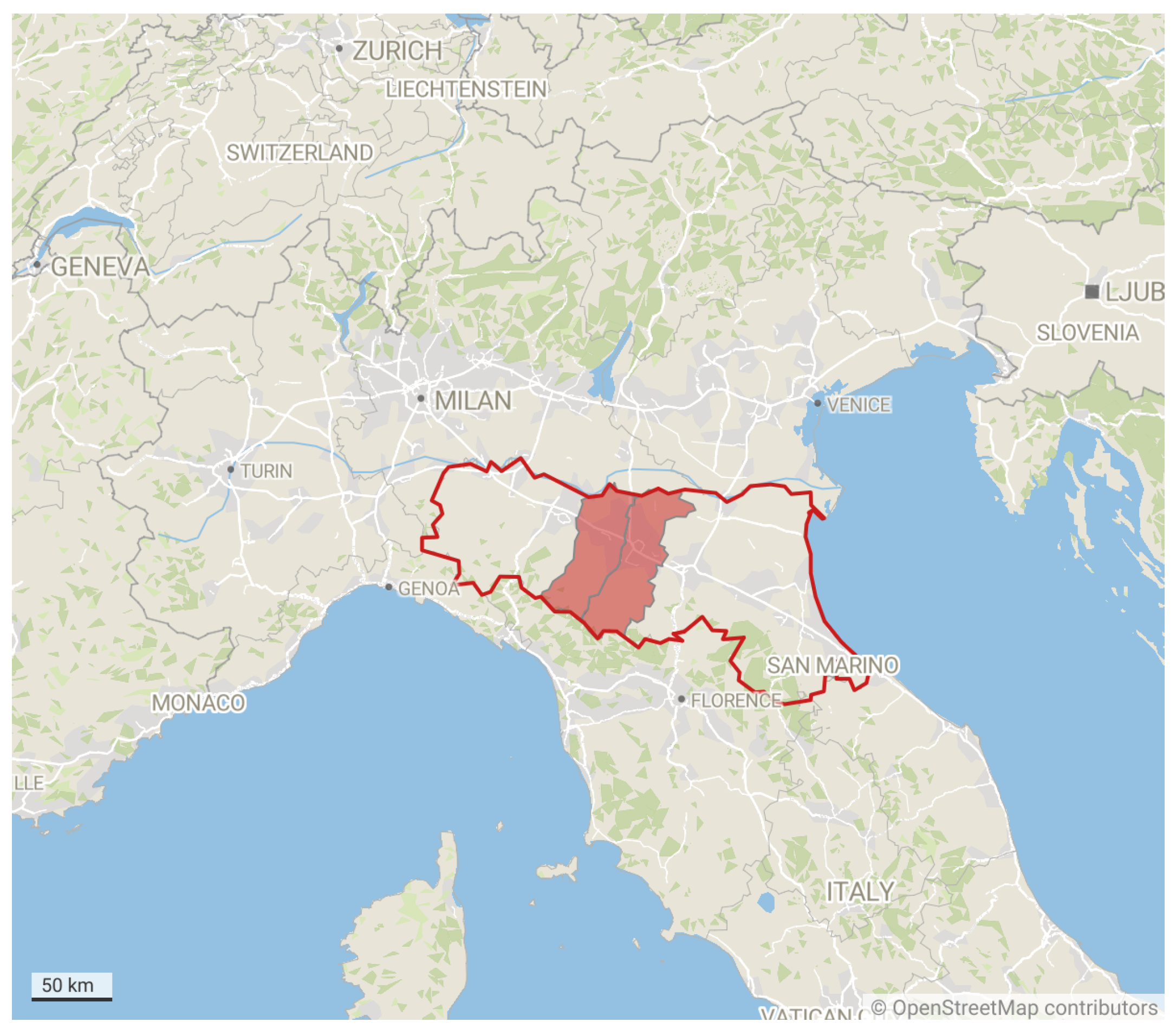
Our case study is situated in the countryside between Modena and Reggio Emilia (Figure 2). This distinctive region is interesting for the following key reasons: (1) The region has significant potential for biogas production, especially from agri-food sector waste, which is plentiful in Emilia-Romagna due to Parmigiano-Reggiano cheese and farming [40]. (2) The region’s agricultural activities generate a substantial amount of biomass, including crop residues, animal manure, food and agro-industrial wastes, and organic waste [41]. (3) Emilia-Romagna has adopted a Regional Energy Plan (REP) to 2030, aiming at greenhouse gas (GHG) emissions reduction, energy consumption control, and enhanced use of bioenergy. This plan, along with Italy’s incentives for renewable energy initiatives, enhances the supply chain’s economic viability [42]. The REP forecasts a notable growth in biogas production, with the possibility of expanding the current installed capacity of 234 MW to 320 MW [40].

This study spans a 10-year time horizon and utilises feedstock composed of agricultural waste and biomass sourced from local communities. The annual amount of this feedstock is determined by calculating the recoverable organic and green fraction of waste from various towns, using per capita waste data, adding sewage and manure data from nearby cow farms. Consequently, each source provides quantities varying between 300 and 9000 t/y (feedstock availability is reported in

Table 2. Amount of feedstocks in each location and period (in t/y).

Source	T1 2	T2	T3	T4	T5	T6	T7	T8	T9	T10
F1 1	3715	3550	3630	3710	3595	3715	3895	3955	3885	3820
F2	1415	1425	1480	1370	1355	1425	1490	1475	1500	1405
F3	770	875	830	800	865	835	890	820	825	855
F4	685	695	730	680	730	695	715	715	710	675
F5	690	635	705	695	675	635	705	635	655	685
F6	4510	4510	4520	4495	4500	4540	4530	4535	4550	4505
F7	490	495	495	460	510	470	505	490	480	510
F8	325	325	330	325	325	335	325	335	320	340
F9	375	350	360	355	375	340	335	345	355	345
F10	340	335	355	340	340	345	340	345	340	350
F11	3940	3955	4195	4195	4140	4125	4170	4160	3825	4005
F12	595	615	625	665	625	640	580	630	640	600
F13	580	625	625	610	605	595	585	565	570	610
F14	445	460	455	420	445	470	480	480	455	465
F15	560	570	575	575	560	565	590	570	570	550
F16	330	335	360	365	345	355	335	350	350	345
F17	2325	2355	2350	2350	2340	2355	2345	2350	2365	2350
F18	320	315	330	310	325	330	325	330	330	350
F19	8810	8820	8815	8820	8810	8805	8810	8815	8820	8810
F20	290	270	265	275	285	285	280	255	285	285

¹ F: Feedstock Source. ² T: Time Period.

).

Three increasing in size PVs are taken into account. It is assumed that all these PVs share the same electricity generation efficiency of 0.14. Information regarding the yearly solar radiation for these facilities is sourced from the PVGIS database [43]. We consider 10 potential sites for anaerobic digestors to process the feedstock. These sites are selected considering their proximity to feedstock sources. Each potential site can host an AD with a capacity ranging from 30,000 to 75,000 t/y. The investment cost for building an AD ranges from EUR 500,000 to EUR 3,000,000, depending on the capacity and site-specific installation costs [44]. The model assumes a biogas yield of 150 Sm₃/t and a fertiliser yield of 200 kg/t of feedstock. The biogas produced by the digestors can be used to generate heat and electricity in cogeneration units. Processing 1000 tonnes of organic waste using an AD typically creates about 20 direct jobs in the sectors of waste collection and management. Furthermore, it leads to an additional 15 jobs indirectly, encompassing roles in the supply chain and various support services [45]. CHPPs vary in capacity between 1 to 20 MW. Their investment costs also differ, ranging from EUR 650,000 to EUR 15,000,000, which can be attributed to variations in scale and technological differences. These systems are characterised by an efficiency of 50% for heat conversion and 30% for electricity generation. Our model includes the integration of ten potential sites for alkaline electrolysers (AEL). Currently, AELs represent the most advanced and cost-efficient technology available for hydrogen production. These units are specifically designed to utilise excess electricity generated by cogeneration systems. The capacity of these electrolysers varies, ranging from 500 kW to 5 MW, with a maximum production rate of 5.5 Sm³H₂/kWh. The investment required for these electrolysers falls between EUR 500,000 and EUR 3,000,000 [46].

Table 3. Technical and economic parameters of different level facilities.

			Small	Medium	Large
PV	Area size	m2	2000	5000	8000
	Power Capacity	MW	0.2	0.7	1.1
	Capacity Factor	-	0.14	0.14	0.14
	Capital Cost	M€	0.4	1	1.6
AD	Capacity	t/y	30,000	50,000	75,000
	Biogas Yield	Nm3/t	50	50	50
	Fertiliser Yield	kg/t	100	100	100
	Capital Cost	M€	0.5	1.5	3
	Emission Factor	kgCO2eq/kg	1.90	1.90	1.90
CHPP	Capacity	MW	1	10	20
	Heat Efficiency	-	0.5	0.5	0.5
	Power Efficiency	-	0.3	0.3	0.3
	Capital Cost	M€	0.65	8	15
	Emission Factor	kgCO2eq/kWh	0.14	0.14	0.14
AEL	Capacity	MW	0.5	2.5	5
	Hydrogen Yield	Sm3H2/kWh	5.5	5.5	5.5
	Capital Cost	M€	0.5	1	3

in the document provides a summary of the key input data for the case study. Hydrogen transportation is accounted for considering a heavy duty truck 30 L/km average consumption and 1.7 €/L gas price. The capacity of trucks for transportation is set with specific limits: trucks are assumed to carry a maximum of 14 tons of biomass and up to 3000 Nm³ of biogas. Revenue generation within the supply chain comes from several sources: fertiliser sales at a unit price of 6 EUR/t, electricity at 0.157 EUR/kWh, heat at 0.075 EUR/kWh, and hydrogen at 5 EUR/Sm³ [47,48].

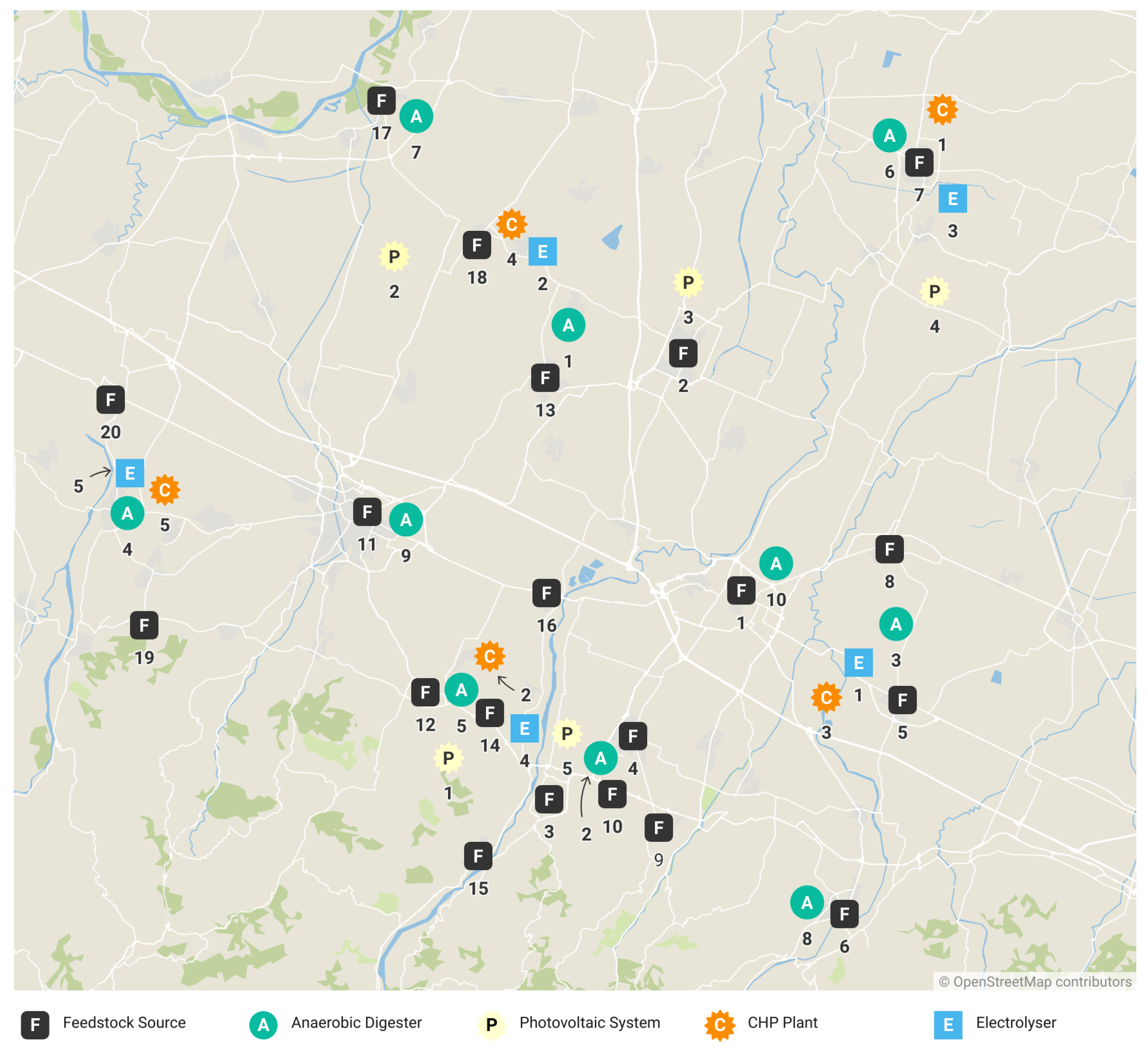
Additionally, the model incorporates emission factors to assess the environmental impact of the supply chain. Various emission factors are included, such as 1.9 kgCO₂eq/kg for anaerobic digestion, 4.20 kgCO₂eq/kgN for fertiliser production, 0.548 kgCO₂eq/kWh for electricity emissions in northern Italy, and 0.137 kgCO₂eq/kWh for cogeneration. In Figure 3, a map is presented of potential facilities sites and feedstock sources. The black “F” symbol represents a feedstock source, the green “A” symbol an AD location, the yellow “P” symbol a PV location, the orange “C” symbol a CHPP location, and the blue “E” symbol an AEL location.

5. Results and Sensitivity Analysis

We will now illustrate how our formulated model is tested using the Emilia Romagna biowaste case study. Model validation is carried out on an Apple M1 Pro with installed 16.00 GB RAM, with a time limit for each run of 3600 s. Initially, we solve each objective function as an individual optimisation model to determine the ideal and anti-ideal solutions based on the case study data (i.e., maximising and minimising each objective function). A linear normalisation technique is employed to transform units of each objective function, obtained from solving the problem, into numerical values that lie between 0 and 1. Subsequently, a weighted sum method is used to convert the multi-objective optimisation model into a single objective function with weighted factors, as depicted in Equation (43). Here, each weight value, w, corresponds to a specific objective function.

$$\begin{array}{c}\hfill min{Z}^{WSM}=-w_1\frac{Z_1-A{I}_1}{I_1-A{I}_1}+w_2\frac{A{I}_2-Z_2}{A{I}_2-I_2}-w_3\frac{Z_3-A{I}_3}{I_3-A{I}_3}\end{array}$$

(43)

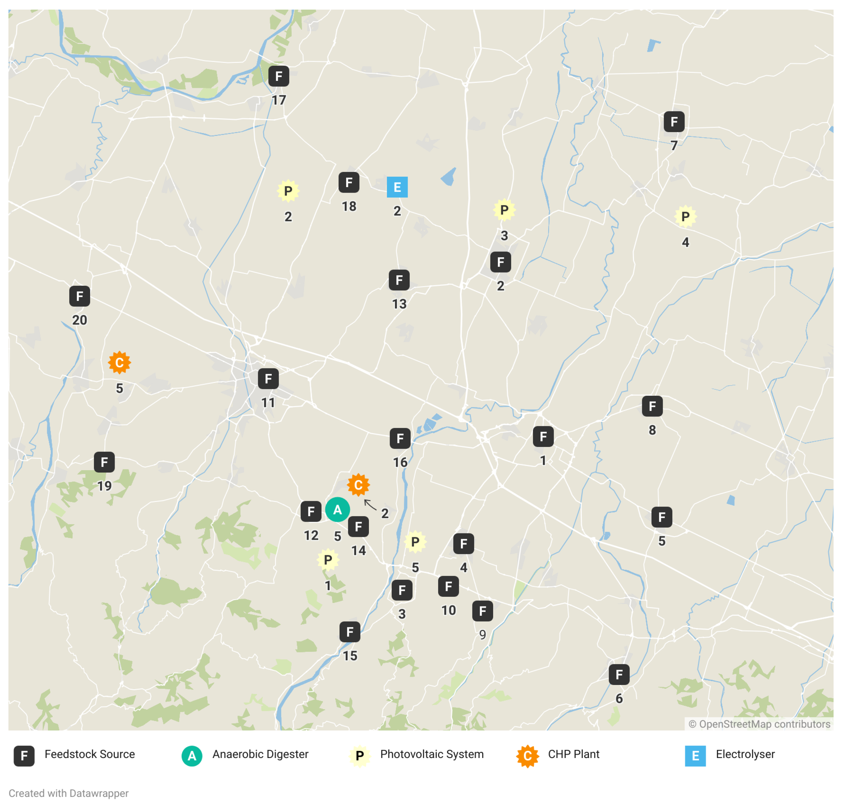
Moreover, the weights are evenly distributed (each set to 1/3) across the economic, social, and environmental dimensions. This allocation underscores the equal significance of each dimension, facilitating the exploration of a hypothetical scenario where all elements are prioritised equally. The results and a map of the selected locations are shown in

Table 4. Key results for each configuration.

	${\mathit{Z}}_1$	${\mathit{Z}}_2$	${\mathit{Z}}_3$	Equal Weights	B-BWM Weights
Ideal Values	637.32 M€	−198.70 ktCO2eq	2660	-	-
(Anti-Ideal Values)	−697.65 M€	0.17 ktCO2eq	-	-	-
Investment Costs	17.65 M€	210.50 M€	313.00 M€	18.15 M€	18.65 M€
Operation Costs	21.69 M€	258.69 M€	384.65 M€	22.31 M€	22.92 M€
Transport Costs	6.13 M€	11.96 M€	-	47.10 M€	60.66 M€
Revenues Total	679.31 M€	238.29 M€	-	679.31 M€	679.31 M€
CF * Transport	0.12 ktCO2eq	0.09 ktCO2eq	-	0.32 ktCO2eq	0.16 ktCO2eq
CF Biogas	2.84 ktCO2eq	2.84 ktCO2eq	-	2.84 ktCO2eq	2.84 ktCO2eq
CF Landfill	-	-	0.17 ktCO2eq	-	-
CF Avoided	−201.62 ktCO2eq	−201.62 ktCO2eq	-	−201.62 ktCO2eq	−201.62 ktCO2eq
Job Employment	276	1947	2660	268	286

* CF: Carbon Footprint.

and Figure 4, following Figure 3 symbols code. In particular, a single AD facility with 50,000 t/y capacity is selected. Additionally, two cogeneration units with a capacity of 1 MW, all five large scale photovoltaic systems, and a single 500 kW electrolyser are selected.

B-BWM is utilised to evaluate the sustainability weights within a collective decision-making framework, where various stakeholders (i.e., managers, public administration, academics), each holding distinct viewpoints, deliberate on which side should be stressed. Best-to-others and others-to-worst tables are presented in

Table 5. B-BWM experts’ judgements.

Expert	Criteria	Vector	Eco	Env	Soc
1	Best: Eco	BtO	1	9	3
	Worst: Env	OtW	9	1	6
2	Best: Eco	BtO	1	6	3
	Worst: Env	OtW	5	1	2
3	Best: Soc	BtO	6	4	1
	Worst: Eco	OtW	1	2	5
4	Best: Env	BtO	3	1	8
	Worst: Soc	OtW	5	9	1
5	Best: Env	BtO	2	1	9
	Worst: Soc	OtW	8	9	1

Notes: BtO: Best-to-Others, OtW: Others-to-Worst.

. The economic dimension is clearly given priority over other dimensions by the first two experts; nevertheless, the second expert exhibits a minor difference in the criteria used. This suggests a balanced approach, valuing economic factors while still giving reasonable weight to environmental and social sustainability. Only the third expert places a strong emphasis on social aspects, indicating a focus on employment-related factors. The final two experts assign significant importance to environmental factors, underscoring a robust commitment to ecological and environmental sustainability.

The social, environmental, and economic aspects of the sustainability paradigm are assigned scores with weights of 0.424, 0.304, and 0.271, respectively, according to the group decision-making analysis. The results in Figure 5 (using the same symbol code as in Figure 3 and Figure 4) suggest the selection of the same AD as previously identified but with the minimal capacity, coupled by an additional facility of medium size. Furthermore, an electrolyser of small size has been chosen at a distinct location. The B-BWM solution highlights the model’s capacity to intricately balance economic, environmental, and social objectives rather than an equal weights solution. Investment costs experience a slight increase under B-BWM conditions (EUR 18.65M) compared with equal weights (EUR 18.15M), indicating a marginal rise in initial investment. Operational costs also experience a slight increase under B-BWM weights (EUR 22.92M versus EUR 22.31M), suggesting that achieving operational efficiency with the B-BWM optimisation incurs a minor cost premium, while transport costs are significantly higher (EUR 60.66M versus EUR 47.10M). Both configurations generate identical revenues (EUR 679.31M) and achieve the same reduction in carbon footprint (−201.62 ktCO₂eq). There is a slight increase in job creation with B-BWM weights (286) compared with equal weights (268), highlighting the social sustainability benefits of the B-BWM-optimised solution, despite the lower allocation weight for B-BWM (0.271 vs. 0.333). The B-BWM-optimised solution balances economic costs, environmental benefits, and social impacts. This approach slightly increases the investment and operational costs but leads to improved sustainability outcomes. In addition, it generates more job positions than equal weights scenario.

When considering the integration of renewable energy sources into UIS models, several critical factors must be addressed. Potential obstacles on the path to implementation warrant careful consideration, including multiple stakeholder engagement and physical constraints. An initial phase of engaging stakeholders and exchanging information will foster robust collaboration between companies and the urban population. This effort should be supported by the involvement of municipal bodies and “facilitators” from industrial districts.

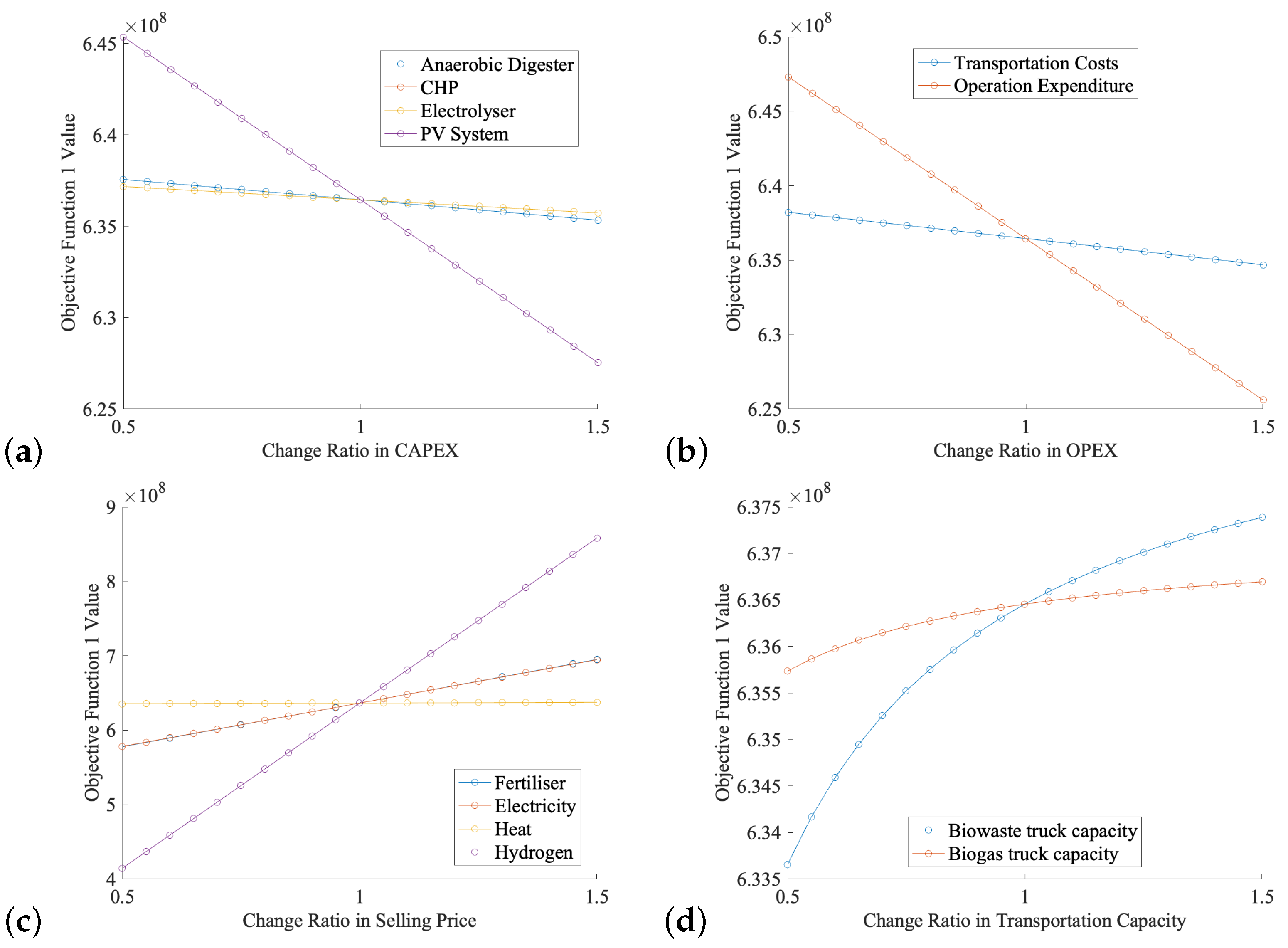
This study focused on examining four critical parameters likely to influence the net present value: capital investment, operational costs, revenue from sales, and transportation capabilities. The objective of the sensitivity analysis was to determine the impact of variations in these parameters on the optimisation results by adjusting them over a predefined range (specifically, from 0.5 to 1.5 times their original values in increments of 0.1). The investigation offered valuable perspectives on the robustness and reactivity of the optimisation model, revealing the impact of various components on the overall outcomes. A cautious assessment of these elements is crucial when determining the economic viability of the project. Figure 6a demonstrates that while investment costs (CAPEX) generally have a moderate impact on the objective function, this is not the case for PVs, which exhibit a significant influence. The sensitivity of PVs indicates a more pronounced response to changes in investment costs, highlighting their crucial role in the overall economic performance of the project. Conversely, Figure 6b depicts the sensitivity of the objective function to alterations in the operation and transport costs. Notably, the objective function’s value exhibits a sharp decline as the operation cost ratio (calculated on a CAPEX basis) expands. Furthermore, Figure 6c examines the effects of changes in the selling prices of commodities produced in the UIS. An increase in the hydrogen price is seen as the most impacting change. Finally, Figure 6d displays a parabolic trend in response to adjustments in the truck capacity for biowaste and biogas. This pattern indicates a diminishing impact on the overall profitability of the project.

Building on the discussed points, it is essential for organisations to make strategic decisions to manage and optimise their investment costs effectively. This involves looking for cost-effective equipment, exploring various suppliers, and negotiating better prices. Moreover, sensitivity to OPEX emphasises the need for efficient operational management to maintain system viability. Additionally, considering geopolitical factors is also important. The selling price of hydrogen is critical and should be monitored closely as market conditions evolve. To reduce operational costs, exploring different transportation options and securing competitive rates is key. Logistics and transportation capacities are pivotal and require strategic planning to ensure they do not become bottlenecks. These steps are crucial for improving cost efficiency and enhancing the effectiveness of waste management processes.

6. Discussion

A significant dependency on weight selection is one of the main drawbacks of weighted sum approaches for resolving multi-objective problems. A linear weighted sum cannot find optimal solutions if the solution functions exhibit a concave trade-off surface [49]. Therefore, an in-depth analysis is performed to investigate the trade-offs between various sets of objective functions. Increasing the importance of one goal function could mean decreasing the efficacy of another. Here, the Pareto front is a useful tool for visualising these inter-dependencies. An efficient frontier is defined as the set of all optimal points [37]. This term indicates a situation in which it is impossible to redistribute resources to benefit one party without harming the benefits of others. The methodology used to solve this model employs an $ϵ$-constraint approach. This technique facilitates the determination of an array of efficient solutions.

$$\begin{array}{cc}\hfill Optimise& o_i\left(\overrightarrow{x}\right)\hfill \end{array}$$

(44)

$$s.t.\left(12\right) - \left(40\right)$$

(45)

$$\begin{array}{cc}\hfill o_j\left(\overrightarrow{x}\right)& \le {ϵ}_{j}j=1,\dots ,kandi\ne j\hfill \end{array}$$

(46)

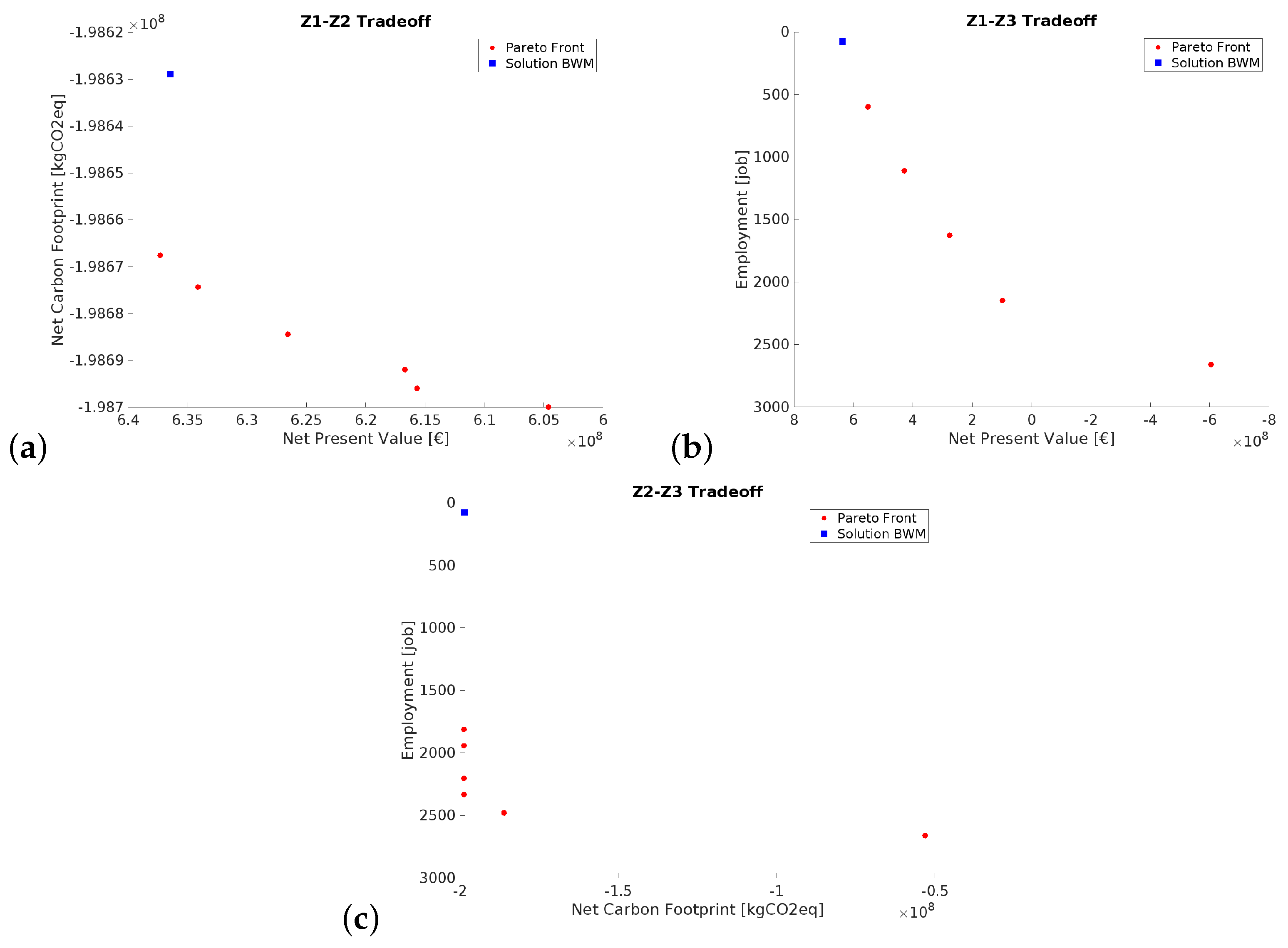
In this research, bi-dimensional graphs are exploited to show trade-offs between various pairs of objective functions, as reported in Figure 7. Figure 7a delineates the trade-off between the economic objective (i.e., net present value) against the social aspect (i.e., expected employment). Figure 7b presents the interplay between the economic (i.e., net present value) and environmental (i.e., carbon footprint) objectives, while Figure 7c examines the interaction between social (expected employment) and environmental (carbon footprint) objectives. As presented, we expect the B-BWM solution to be located in the upper left side of the graph, reflecting the prioritisation of economic, environmental, and social objectives in the assigned weights. Moreover, the axes in these graphical representations are reversed to align the visual depiction with standard interpretations. This manipulation ensures that the direction indicative of preferable outcomes remains consistent across all plots, thereby enhancing the intuitive understanding of the trade-offs being visualised.

In this section, we present specific recommendations for better understanding the trade-offs among economic, environmental, and social objectives. Managers should carefully consider the relative importance of economic, environmental, and social goals in their operational context to guide the optimisation process effectively. The $ϵ$-constraint approach suggests a dependency between the net present value and the carbon footprint; in fact, the B-BWM solution produces very high avoided emissions due to the efficient exploitation of waste. However, the Pareto front, with $Z_1$ as the primary function, demonstrates limited savings even for higher net carbon footprints. Enhancing one objective might compromise another, and thus, aiming for an optimal balance is essential. Prioritising job creation could result in excessive costs, while simultaneously offering limited environmental benefits. The B-BWM-based weighted sum approach represents a sufficiently good and feasible solution for balancing stakeholders’ preferences, as it facilitates job creation without adversely affecting economic and environmental objectives. Simultaneously, it provides a sustainable solution from both environmental and economic perspectives.

7. Conclusions

This study focused on creating a supply chain framework for an energy symbiosis system in Emilia-Romagna, focusing on the conversion of biomass into biogas, heat, electricity, and green hydrogen through electrolysis. This approach promotes sustainable development by leveraging resource exchanges between industrial, urban, and rural sectors. The model also integrates the use of by-products, especially fertilisers from ADs, to enhance both economic and environmental impacts. Key to this model is the development of a hydrogen supply chain, marking a significant step towards sustainable energy systems. This initiative addresses the crucial challenge of economic viability, proposing a gradual transition that starts with hydrogen integration into existing natural gas infrastructures and progresses towards electrolysis powered by renewable sources. This strategy is particularly vital for heavy transport and industries that are challenging to decarbonise. The study underscores the importance of effective municipal and rural waste management and the establishment of a proficient hydrogen supply chain as central to the region’s stakeholders. By capitalising on the benefits of green hydrogen, which contributes significantly less to global warming compared to traditional hydrogen production methods, the model sets a path towards low-carbon mobility and industrial synergy. In UIS settings, renewable energy sources present an opportunity to lower GHG emissions, fight climate change, and foster a more sustainable future. The proposed supply chain model incorporates aspects such as feedstock supply, multi-energy systems, and multiple energy carriers to enhance the efficiency of the biomass-to-energy and biomass–hydrogen networks.

By addressing a multi-objective optimisation problem, the model offers a comprehensive approach to maximise the economic net present value, minimise environmental impact, and boost job creation. The optimisation problem is addressed using a weighted sum method with B-BWM for preference articulation. This method is enhanced by the linear normalisation technique, which standardises the objective function values for comparability. The B-BWM is characterised by its efficiency and reduced bias in decision-making, involving a detailed comparison process between the best and worst criteria. It facilitates sensitivity studies, allowing stakeholders to evaluate the effects of various factors on the final results. The results show that applying the B-BWM to solve the multi-objective optimisation in our case study yields positive economic impacts, with high overall revenues of EUR 679.31M, while keeping costs limited to investments (EUR 18.65M), operations, and transportation. On the other hand, the carbon footprint from landfilling and primary energy production is reduced, considering an increase in biogas production and transportation efficiency. Finally, job employment is boosted by the opening of AD, CHPP, and AEL facilities.

In terms of the limitations of this research, scalarisation methods in multi-objectives may lead to solutions that are biased towards objectives with higher assigned weights. This is why we opted to previously perform a weighting phase with a group decision-making method to balance diverse stakeholders’ perspectives. Additionally, this method might not fully explore the Pareto front, particularly its non-convex regions. This is why we employed a $ϵ$-constrain method to visualise the trade-offs and compare them to our proposed solution. Nonetheless, other a priori multi-objective approaches can be explored. It is important to note that the conducted sensitivity analysis does not consider how variables may change over time; simulation studies in the solution could offer more detailed analysis of system sensitivity. Moreover, due to computational limitations (owing to the high number of parameters), it was not possible to test inter-dependencies.

This study provides valuable insights into the economic, operational, and environmental aspects of the biomass-to-energy and biomass-to-hydrogen supply chain. However, future research could focus on incorporating uncertainty by developing a stochastic model since uncertainty exists for various supply chain echelons (e.g., demand fluctuations, supply interruptions, lead time variability, price volatility, taxation, subsidies, technological innovations, and unforeseen disruptive events like natural disasters). The impact of such uncertainties can significantly disrupt the supply chain, affecting each echelon from feedstock availability to biogas and energy supply. To enhance resilience against these uncertainties, future models would benefit from including proactive and reactive strategies, such as facility fortification, backup supplies, and redundancy. Additionally, incorporating other social and environmental factors would provide a more holistic view of the supply chain dynamics. Social factors may relate to labour conditions and community impact, particularly concerning health and safety. While other environmental factors can integrate life cycle assessment indicators. Employing spatial analysis alongside MCDM approaches could significantly enhance the capabilities for optimal location selection, ensuring a more efficient and sustainable biomass-to-energy supply chain. Finally, analysis of policy scenarios could facilitate improved judgement regarding taxation and the dynamics of technological innovation.

References

- Lee, H.; Calvin, K.; Dasgupta, D.; Krinner, G.; Mukherji, A.; Thorne, P.; Trisos, C.; Romero, J.; Aldunce, P.; Barrett, K.; et al. IPCC, 2023: Summary for Policymakers. In Climate Change 2023: Synthesis Report. Contribution of Working Groups I, II and III to the Sixth Assessment Report of the Intergovernmental Panel on Climate Change; Core Writing Team, Lee, H., Romero, J., Eds.; IPCC: Geneva, Switzerland, 2023; pp. 1–34. [Google Scholar] [CrossRef]
- Silva, M.G.; Przybysz, A.L.; Piekarski, C.M. Location as a key factor for waste to energy plants. J. Clean. Prod. 2022, 379, 134386. [Google Scholar] [CrossRef]
- Lo Monaco, A.; Mallegni, R. La Gestione Dei Rifiuti in Emilia-Romagna: Report 2022; Pazzini Stampatore Editore S.r.l.: Villa Verrucchio, Italy, 2023; Technical Report, Regione Emilia-Romagna, Arpae Emilia-Romagna. [Google Scholar]
- Beyene, H.; Werkneh, A.; Ambaye, T. Current Updates on Waste to Energy (WtE) Technologies: A Review. Renew. Energy Focus 2018, 24, 1–11. [Google Scholar] [CrossRef]
- Rasheed, T.; Anwar, M.; Ahmad, N.; Sher, F.; Khan, S.D.; Ahmad, A.; Khan, R.; Wazeer, I. Valorisation and Emerging Perspective of Biomass Based Waste-to-Energy Technologies and Their Socio-Environmental Impact: A Review. J. Environ. Manag. 2021, 287, 112257. [Google Scholar] [CrossRef]
- Ferraz de Campos, V.; Silva, V.; Cardoso, J.; Brito, P.; Tuna, C.; Silveira, J. A Review of Waste Management in Brazil and Portugal: Waste-to-energy as Pathway for Sustainable Development. Renew. Energy 2021, 178, 802–820. [Google Scholar] [CrossRef]
- Malode, S.; Prabhu, K.; Mascarenhas, R.; Shetti, N.; Aminabhavi, T. Recent Advances and Viability in Biofuel Production. Energy Convers. Manag. X 2021, 10, 100070. [Google Scholar] [CrossRef]
- Khan, I. Waste to Biogas through Anaerobic Digestion: Hydrogen Production Potential in the Developing World—A Case of Bangladesh. Int. J. Hydrogen Energy 2020, 45, 15951–15962. [Google Scholar] [CrossRef]
- Lepage, T.; Kammoun, M.; Schmetz, Q.; Richel, A. Biomass-to-Hydrogen: A Review of Main Routes Production, Processes Evaluation and Techno-Economical Assessment. Biomass Bioenergy 2021, 144, 105920. [Google Scholar] [CrossRef]
- OECD. Global Hydrogen Review 2021; Organisation for Economic Co-Operation and Development; IEA: Paris, France, 2023. [Google Scholar]
- Cho, H.H.; Strezov, V.; Evans, T.J. A Review on Global Warming Potential, Challenges and Opportunities of Renewable Hydrogen Production Technologies. Sustain. Mater. Technol. 2023, 35, e00567. [Google Scholar] [CrossRef]
- Koroneos, C.; Dompros, A.; Roumbas, G. Hydrogen Production via Biomass Gasification—A Life Cycle Assessment Approach. Chem. Eng. Process. Process Intensif. 2008, 47, 1261–1268. [Google Scholar] [CrossRef]
- Wilkinson, J.; Mays, T.; McManus, M. Review and Meta-Analysis of Recent Life Cycle Assessments of Hydrogen Production. Clean. Environ. Syst. 2023, 9, 100116. [Google Scholar] [CrossRef]
- Butturi, M.A.; Gamberini, R. Urban–Industrial Symbiosis to Support Sustainable Energy Transition. Int. J. Energy Prod. Manag. 2020, 5, 355–366. [Google Scholar] [CrossRef]
- Chertow, M.R. Industrial symbiosis: Literature and taxonomy. Annu. Rev. Energy Environ. 2000, 25, 313–337. [Google Scholar] [CrossRef]
- Lombardi, D.R.; Laybourn, P. Redefining industrial symbiosis: Crossing academic-practitioner boundaries. J. Ind. Ecol. 2012, 16, 28–37. [Google Scholar] [CrossRef]
- Mortensen, L.; Kørnøv, L. Critical factors for industrial symbiosis emergence process. J. Clean. Prod. 2019, 212, 56–69. [Google Scholar] [CrossRef]
- Chertow, M.; Ehrenfeld, J. Organizing self-organizing systems: Toward a theory of industrial symbiosis. J. Ind. Ecol. 2012, 16, 13–27. [Google Scholar] [CrossRef]
- Turken, N.; Geda, A. Supply chain implications of industrial symbiosis: A review and avenues for future research. Resour. Conserv. Recycl. 2020, 161, 104974. [Google Scholar] [CrossRef]
- Butturi, M.A.; Gamberini, R. The Potential of Hydrogen Technologies for Low-Carbon Mobility in the Urban–Industrial Symbiosis Approach. Int. J. Energy Prod. Manag. 2022, 7, 151–163. [Google Scholar] [CrossRef]
- Neves, A.; Godina, R.; Azevedo, S.G.; Matias, J.C. A comprehensive review of industrial symbiosis. J. Clean. Prod. 2020, 247, 119113. [Google Scholar] [CrossRef]
- Kim, J.; Realff, M.J.; Lee, J.H.; Whittaker, C.; Furtner, L. Design of biomass processing network for biofuel production using an MILP model. Biomass Bioenergy 2011, 35, 853–871. [Google Scholar] [CrossRef]
- Gondal, I.A.; Sahir, M.H. Model for biomass-based renewable hydrogen supply chain. Int. J. Energy Res. 2013, 37, 1151–1159. [Google Scholar] [CrossRef]
- Balaman, S.Y.; Selim, H. A Network Design Model for Biomass to Energy Supply Chains with Anaerobic Digestion Systems. Appl. Energy 2014, 130, 289–304. [Google Scholar] [CrossRef]
- Patrizio, P.; Leduc, S.; Chinese, D.; Dotzauer, E.; Kraxner, F. Biomethane as transport fuel—A comparison with other biogas utilization pathways in northern Italy. Appl. Energy 2015, 157, 25–34. [Google Scholar] [CrossRef]
- Wu, B.; Sarker, B.R.; Paudel, K.P. Sustainable energy from biomass: Biomethane manufacturing plant location and distribution problem. Appl. Energy 2015, 158, 597–608. [Google Scholar] [CrossRef]
- Mayerle, S.F.; de Figueiredo, J.N. Designing optimal supply chains for anaerobic bio-digestion/energy generation complexes with distributed small farm feedstock sourcing. Renew. Energy 2016, 90, 46–54. [Google Scholar] [CrossRef]
- Woo, Y.B.; Cho, S.; Kim, J.; Kim, B.S. Optimization-Based Approach for Strategic Design and Operation of a Biomass-to-Hydrogen Supply Chain. Int. J. Hydrogen Energy 2016, 41, 5405–5418. [Google Scholar] [CrossRef]
- López-Díaz, D.C.; Lira-Barragán, L.F.; Rubio-Castro, E.; Ponce-Ortega, J.M.; El-Halwagi, M.M. Optimal location of biorefineries considering sustainable integration with the environment. Renew. Energy 2017, 100, 65–77. [Google Scholar] [CrossRef]
- Silva, S.; Alçada-Almeida, L.; Dias, L.C. Multiobjective programming for sizing and locating biogas plants: A model and an application in a region of Portugal. Comput. Oper. Res. 2017, 83, 189–198. [Google Scholar] [CrossRef]
- Han, S.; Kim, J. A multi-period MILP model for the investment and design planning of a national-level complex renewable energy supply system. Renew. Energy 2019, 141, 736–750. [Google Scholar] [CrossRef]
- Bijarchiyan, M.; Sahebi, H.; Mirzamohammadi, S. A Sustainable Biomass Network Design Model for Bioenergy Production by Anaerobic Digestion Technology: Using Agricultural Residues and Livestock Manure. Energy Sustain. Soc. 2020, 10, 19. [Google Scholar] [CrossRef]
- Maha, A.X.Y.; Hoa, W.S.; Hassima, M.H.; Hashima, H.; Liewb, P.Y.; Aslia, U.A.; Muisa, Z.A.; Lingc, G.H.T. Optimization of hydrogen supply chain: A case study in Malaysia. Chem. Eng. Trans. 2020, 78, 85–90. [Google Scholar] [CrossRef]
- Thiriet, P.; Bioteau, T.; Tremier, A. Optimization Method to Construct Micro-Anaerobic Digesters Networks for Decentralized Biowaste Treatment in Urban and Peri-Urban Areas. J. Clean. Prod. 2020, 243, 118478. [Google Scholar] [CrossRef]
- Rahimi, T.; Babazadeh, R.; Doniavi, A. Designing and Planning the Animal Waste-to-Energy Supply Chains: A Case Study. Renew. Energy Focus 2021, 39, 37–48. [Google Scholar] [CrossRef]
- Abbasi, G.; Khoshalhan, F.; Javad Hosseininezhad, S. Municipal Solid Waste Management and Energy Production: A Multi-Objective Optimization Approach to Incineration and Biogas Waste-to-Energy Supply Chain. Sustain. Energy Technol. Assess. 2022, 54, 102809. [Google Scholar] [CrossRef]
- Marler, R.T.; Arora, J.S. Survey of multi-objective optimization methods for engineering. Struct. Multidiscip. Optim. 2004, 26, 369–395. [Google Scholar] [CrossRef]
- Rezaei, J. Best-worst multi-criteria decision-making method. Omega 2015, 53, 49–57. [Google Scholar] [CrossRef]
- Mohammadi, M.; Rezaei, J. Bayesian best-worst method: A probabilistic group decision making model. Omega 2020, 96, 102075. [Google Scholar] [CrossRef]
- Mattias, G.; Elena, T.; Giuseppe, C.; Anna, F.E. Modeling the Ecosystem Service of Agricultural Residues Provision for Bioenergy Production: A Potential Application in the Emilia-Romagna Region (Italy). Ecol. Model. 2021, 451, 109571. [Google Scholar] [CrossRef]
- Greggio, N.; Balugani, E.; Carlini, C.; Contin, A.; Labartino, N.; Porcelli, R.; Quaranta, M.; Righi, S.; Vogli, L.; Marazza, D. Theoretical and Unused Potential for Residual Biomasses in the Emilia Romagna Region (Italy) through a Revised and Portable Framework for Their Categorization. Renew. Sustain. Energy Rev. 2019, 112, 590–606. [Google Scholar] [CrossRef]
- Tamburini, E.; Gaglio, M.; Castaldelli, G.; Fano, E.A. Biogas from Agri-Food and Agricultural Waste Can Appreciate Agro-Ecosystem Services: The Case Study of Emilia Romagna Region. Sustainability 2020, 12, 8392. [Google Scholar] [CrossRef]
- Huld, T.; Müller, R.; Gambardella, A. A new solar radiation database for estimating PV performance in Europe and Africa. Sol. Energy 2012, 86, 1803–1815. [Google Scholar] [CrossRef]
- Cecchi, F.; Battistoni, P.; Pavan, P.; Bolzonella, D.; Innocenti, L. Digestione Anaerobica Della Frazione Organica dei Rifiuti Solidi; Technical Report; ISPRA: Rome, Italy, 2005. [Google Scholar]
- Piadeh, F.; Offie, I.; Behzadian, K.; Rizzuto, J.P.; Bywater, A.; Córdoba-Pachón, J.R.; Walker, M. A critical review for the impact of anaerobic digestion on the sustainable development goals. J. Environ. Manag. 2024, 349, 119458. [Google Scholar] [CrossRef] [PubMed]
- Vidas, L.; Castro, R. Recent Developments on Hydrogen Production Technologies: State-of-the-Art Review with a Focus on Green-Electrolysis. Appl. Sci. 2021, 11, 11363. [Google Scholar] [CrossRef]
- Il Mercato del Compost. Available online: https://www.compost.it/il-compost-e-il-marchio-compost-di-qualita-cic/il-mercato-del-compost/ (accessed on 16 May 2023).
- ARERA. Available online: https://www.arera.it/it/index.htm (accessed on 16 May 2023).
- Cho, J.H.; Wang, Y.; Chen, R.; Chan, K.S.; Swami, A. A survey on modeling and optimizing multi-objective systems. IEEE Commun. Surv. Tutor. 2017, 19, 1867–1901. [Google Scholar] [CrossRef]