Deep Ensembles Based on Stochastic Activations for Semantic Segmentation

Abstract

Semantic segmentation is a very popular topic in modern computer vision, and it has applications in many fields. Researchers have proposed a variety of architectures for semantic image segmentation. The most common ones exploit an encoder–decoder structure that aims to capture the semantics of the image and its low-level features. The encoder uses convolutional layers, in general with a stride larger than one, to extract the features, while the decoder recreates the image by upsampling and using skip connections with the first layers. The objective of this study is to propose a method for creating an ensemble of CNNs by enhancing diversity among networks with different activation functions. In this work, we use DeepLabV3+ as an architecture to test the effectiveness of creating an ensemble of networks by randomly changing the activation functions inside the network multiple times. We also use different backbone networks in our DeepLabV3+ to validate our findings. A comprehensive evaluation of the proposed approach is conducted across two different image segmentation problems: the first is from the medical field, i.e., polyp segmentation for early detection of colorectal cancer, and the second is skin detection for several different applications, including face detection, hand gesture recognition, and many others. As to the first problem, we manage to reach a Dice coefficient of 0.888, and a mean intersection over union (mIoU) of 0.825, in the competitive Kvasir-SEG dataset. The high performance of the proposed ensemble is confirmed in skin detection, where the proposed approach is ranked first concerning other state-of-the-art approaches (including HarDNet) in a large set of testing datasets.

1. Introduction

Semantic segmentation is a computer vision activity that consists in labeling the pixels of an image with the class they belong to. This has very important applications in many fields such as autonomous driving [1] and computer-aided medical diagnosis [2]. In recent years, deep learning techniques have become the most relevant ones to address this problem. An early architecture for semantic segmentation was U-Net [3], which was based on an encoder-decoder structure. However, it failed to precisely classify the borders of the figures, due to the lack of skip-connections in the decoder. After that, many other segmentation networks were proposed and most of them followed more or less the same structure [4,5,6].

In this paper, we propose a novel approach to image segmentation based on ensembles of DeepLabV3+, which is one of the architectures of the DeepLab family. The motivation of the proposed method is the following: it is well known from the literature that ensemble classifiers can be used for improving prediction performance and in this case the accuracy of segmentation. No single model exists that works well for all the segmentation problems, however, the sets of objects segmented by the different methods would not necessarily overlap, which suggested that different algorithms potentially offered complementary information. This led to the possibility of fusing the responses obtained by different approaches to hopefully gain better performance. To design a good ensemble the classifier diversity is the most important property to be considered, i.e. their capability not to make coincident errors. With the motivation of creating diversity in an ensemble, our approach to segmentation consists in creating an ensemble starting from the same architecture, but randomly substituting its activation functions. Given a base segmentation model, which consists of the DeepLabV3+ architecture in our case, first, we evaluate the use of different backbone networks (i.e. ResNet, Xception, EfficentNet, and MobileNet), to select the most suited for the given problem, then we stochastically substitute each ReLU activation function, with a random one extracted from a pool of activations proposed in the literature. We aim to show that we can train a large number of high-performing classifiers that are independent enough from each other to be useful when included in an ensemble.

Here we focus on two applications, in particular on colorectal cancer segmentation and skin detection.

Colorectal Cancer is one of the most dangerous cancers according to the statistics. The early diagnosis is crucial to be able to fully remove it while it is small. The presence of polyps in the colon is highly correlated with the appearance of cancer, hence they must be recognized and removed as soon as possible [7]. However, this is a challenging task even for trained doctors, hence an automatic tool able to recognize them would be very useful in this case. The boundaries of polyps are not always easy to recognize, due to their similarity with surrounding mucosa, besides there might be partial occlusions. Polyps belong to four different classes: adenoma, serrated, hyperplastic, and mixed, which is quite rare. This makes classification and detection even harder.

Skin detection is a completely different task when it comes to applications. It is a useful step for face detection, body tracking, and gesture recognition [8,9,10]. However, the deep learning tools, as well as the challenges, are very similar in polyp segmentation and skin detection. Again, we usually face occlusions and intra-class variance, since images have very different light and the subjects can be very different from each other.

The outbreak of deep learning for computer vision led to an increased effort to improve the classification performances of methods for semantic segmentation on a variety of applications. Nowadays state-of-the-art approaches have performances comparable with human experts in polyp segmentation [2,11,12,13]. However, this application has a long history, and the first methods used classic machine learning techniques. For example, Thambawita et al. [14] trained five models for polyp segmentation including both classical machine learning techniques as well as convolutional networks. Guo et al. [15] proposed a couple of fully convolutional networks to participate at the Gastrointestinal Image ANAlysis (GIANA) in 2017 and 2018 and managed to reach the first and second place in the ranking in two consecutive years. Until recently, methods for polyp segmentation were trained and tested on very small datasets, preventing the networks to generalize enough and also not allowing a good statistical significance of the results. Besides, most of the largest datasets were not publicly released [2,11].

Jha et al. [16] recently made available a new public polyp dataset, named Kvasir-SEG dataset, including 1,000 polyp images annotated by expert endoscopists from the Oslo University Hospital. Jha et al. [17] propose a method based on ResNet and U-Net which reached very promising results in this novel dataset.

Skin detection also saw a huge number of papers dealing with this issue both before and after the deep learning revolution. For example, Phung et al. [18] proposed an approach based on classical machine learning techniques such as histograms analysis and Gaussian mixture classifiers. More recently, Roy et al. [19] proposed a system for hand recognition based on skin segmentation using CNNs. Arsalan et al. [20] used a CNN with skip connections for generic skin recognition, following the modern trends that tend to apply skip connections in neural networks more and more often. Shahriar et al. [21] used skin recognition based on CNN to detect hands, to interpret the sign language. Lumini and Nanni [22] performed extensive experiments using several CNN architectures and concluded that DeepLabv3+ gained the best performance for skin segmentation.

In this paper, we propose a framework for designing ensemble classifiers for semantic segmentation. The main contribution of this work is:

A method for increasing classifier diversity where each neural network is stochastically designed by varying the activation layers to increase the diversity of the ensemble. A selection procedure to include in the final set a pool of K networks selected as the most diverse networks on the given problem. The selection procedure is performed using only training data

Extensive experimentations in two very different segmentation problems confirm the good performance of the ensemble. Our approach has been compared with other state-of-the-art methods in both problems, included the recently proposed HarDNet-MSEG [23] which here is evaluated for the first time in the skin detection problem.

2. Methods

2.1. Deep Learning for Semantic Image Segmentation

Image segmentation is a pixel-based classification problem that performs pixel-level labeling with a set of object categories for all image pixels. Fully Convolutional Networks (FNC) [6] are one of the first attempts to use CNN for segmentation: they were designed by replacing the last fully connected layers of a net with a fully convolutional layer that allows the classification of the image on a per-pixel basis.

A step forward in the design of a segmentation network is done by the encoder-decoder architecture [3] which overcomes the loss of information of FNC due to the absence of deconvolution, by proposing an architecture where a multi-layer deconvolution network is learned. A similar architecture is proposed by U-Net, a U-shape network where the encoder part downsamples the image and increases the number of features, while the opposite decoder part increases the image resolution to the input size [24]. Another encoder-decoder structure is proposed in SegNet [4], which uses VGG [25] as a backbone encoder, coupled to a symmetric decoder structure. In SegNet decoding is performed using max-pooling indices from the corresponding encoder layer, as opposed to concatenating it as in U-Net, thus saving memory and getting a better boundary reconstruction.

The next step to image segmentation is represented by DeepLab [26], a semantic segmentation model designed by Google which achieves dense prediction by simply up-sampling the output of the last convolution layer and computing pixel-wise loss. The novelty is in the use of atrous convolution for up-sampling: it is a dilated convolution that uses a dilation rate to effectively enlarge the field of view of filters without increasing the number of parameters or the amount of computation. The last improvement of the DeepLab family is DeepLabV3+ [27], which combines cascaded and parallel modules of dilated convolutions and is the architecture used in this work.

Several other architectures have been proposed in the literature for image segmentation, including recurrent neural networks, attention-based and generative models. The interested reader can refer to [28] for a recent survey.

Apart from the main architecture of the network, there are a handful of other good design choices that would help to achieve good performance. For example, the choice of a pretrained backbone for the encoder part of the network. Among several CNNs [29] widely used for transfer learning we tested the following models (

Table 1. Summary of CNN models.

Network	Depth	Size (MB)	Parameters (Millions)	Input Size
mobilenetv2	53	13	3.5	224 × 224
resnet18	18	44	11.7	224 × 224
resnet50	50	96	25.6	224 × 224
xception	71	85	22.9	299 × 299
IncR	164	209	55.9	299 × 299
efficientnetb0	82	20	5.3	224 × 224

):

• MobileNet-v2 [30] is a lightweight CNN designed for mobile devices based on depthwise separable convolutions.
• ResNet18 and ResNet50 [31] are two CNNs of the ResNet family, a set of architectures based on the use of residual blocks in which intermediate layers of a block learn a residual function concerning the block input.
• Xception [32] is a CNN architecture that relies solely on depthwise separable convolution layers.
• Inception-ResNet-v2 (IncR,) [33] combines the Inception architecture with residual connections. In the Inception-Resnet block, multiple-sized convolutional filters are combined with residual connections, replacing the filter concatenation stage of the Inception architecture.
• EfficentNet [34], is a family of CNNs designed to scale well with performance. EfficientNetB0 is a simple mobile-size baseline architecture, the other networks of the family are obtained applying an effective compound scaling method for increasing the model size to achieve maximum accuracy gains.

Also, the choice of the loss function influences the way the network is trained. The most used loss function for the task of image segmentation is a pixel-wise cross-entropy loss. This loss treats the problem as a multi-class classification problem at pixel level comparing the class predictions to the actual label. Pixel-wise loss is calculated as the log loss summed over all the classes and averaged over all pixels. This can be a problem if some classes have unbalanced representation in the image, as training can be dominated by the most prevalent class. A possible solution is to use weighting for each class to counteract a class imbalance present in the dataset [6].

Another popular loss function for image segmentation is the Dice loss [35], which is based on the Sørensen-Dice similarity coefficient for measuring overlap between two segmented images. This measure ranges from 0 to 1 where a Dice coefficient of 1 denotes perfect and complete overlap. The Dice loss is used in this work. Other popular loss functions for image segmentation and their usage for fast and better convergence of a model are reviewed in [36].

Moreover, the choice of the activation function can be significant. ReLU is the nonlinearity that most works use in the area, but several works have reported improved results with different activation functions [37]. In Section 2.2, our approach for perturbing models by replacing activation layers is explained.

Finally, data augmentation can help avoid overfitting, since in many applications, the size of the dataset is small compared to the number of parameters in a segmentation deep neural network. We perform experiments with data augmentation, consisting of horizontal and vertical flips and rotations of 90°.

2.2. Stochastic Activation Selection

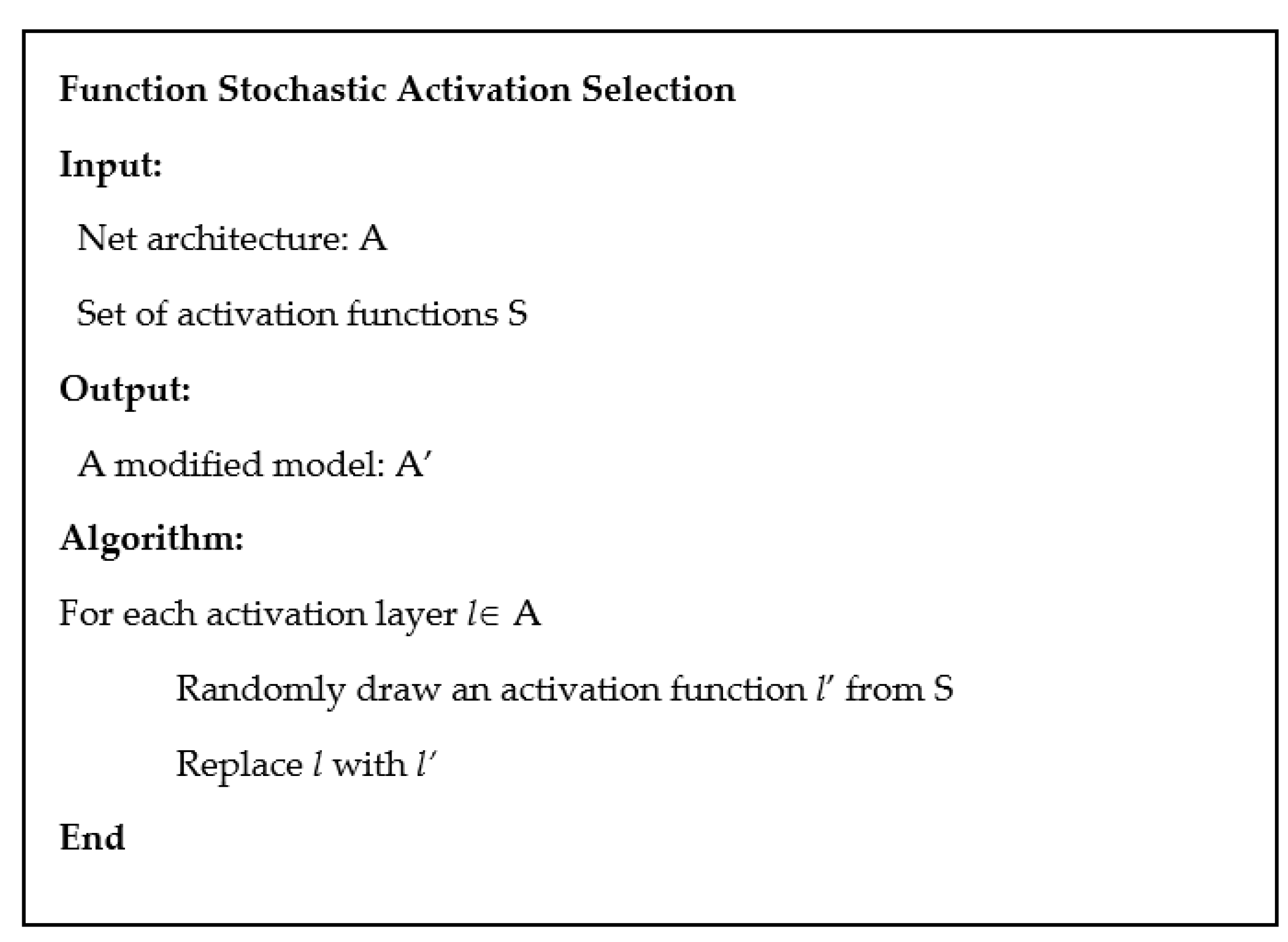
Given a neural network architecture and a pool of different activation functions, Stochastic Activation Selection consists in creating different versions of the same architecture that differ in the choice of the activation layers. This method was first introduced in [37]. The process to create a new network is based on the replacement of each activation layer (ReLU) by a new activation function which can be fixed a priori or randomly selected. This leads to a new network, which in the stochastic version, has different activation layers through the layers. Since this is a random procedure, it yields a different network every time. Hence, we iterate the process multiple times to create many different networks that we use to create an ensemble of neural networks. We train each network independently on the same set of data and then we merge their results using the average rule, which consists in averaging the softmax output of the networks in the ensemble. The pseudo-code of the procedures for stochastic activation selection is reported in Figure 1.

In this paper, we use Deeplabv3+ [27] as neural architecture. The pool of activation functions is made by the following activation functions. ReLU [38] is the most common activation in modern deep learning. Leaky ReLU [39] is a modification of ReLU that has a small positive slope for negative values to avoid zero gradient regions. ELU [40] also has a positive slope for negative values that saturates as the input goes to minus infinity. PReLU [41] is a leaky ReLU whose slopes on negative values are different in every channel and are learnable. S-Shaped ReLU [42] (SReLU), as its name suggests, has the shape of the letter S, since it is equal to the identity function in a compact interval that contains zero and has a learnable slope outside the interval. This introduces further representation power to the activation. Adaptive Piecewise Linear Unit [43] (APLU) goes deeper in this direction since its learnable parameters are all the non-differentiability points and the slopes of a generic piecewise linear function with a fixed number of non-differentiability points. Mexican ReLU [44] (MeLU) (with $k\in \left\{4,8\right\}$) is similar to APLU, since it is a generic piecewise linear function, although non-differentiability points are fixed and the different slopes are obtained by adding triangular function (Mexican hat functions) to leaky ReLU. This allows a more stable training. Gaussian Linear Unit (GaLU) [37] (with $k\in \left\{4,8\right\}$) follows the idea of MeLU but adding Gaussian-like function, PDELU is a smooth function equal to ReLU for positive values and whose slope on positive values is calculated so that its output has zero mean and unit variance if the input follows a Gaussian distribution with zero mean and unit variance [45]. Swish (fixed and learnable) is an activation introduced in [46] using a random search and reinforcement learning to find the “optimal” activation function, Soft Root Sign [47] is similar to PDELU in the sense that is the function that maps a standard Gaussian into a random variable with unit mean-variance. Mish (fixed and learnable) [48] is defined as

$$f\left(x\right)=x·\tan \mathrm{h}\left(\log \left(1+e^{ax}\right)\right)$$

and their authors report very high performances for this function that rapidly goes to minus infinity for small values, as it does not happen often for activation functions. Lastly, Soft Learnable [37] is yet another function that maps Gaussian distributions into zero mean and unit variance distributions.

3. Results on Colorectal Cancer Segmentation

3.1. Datasets, Testing Protocol, and Metrics

All the experiments on colorectal cancer segmentation have been carried out on the Kvasir-SEG dataset [16] which includes 1000 polyp images acquired by a high-resolution electromagnetic imaging system, with a ground-truth consisting of bounding boxes and segmentation masks. For a fair comparison with other approaches as [17,23] we use the following testing protocol: 880 images are used for training and the remaining 120 for testing.

The image sizes varied between 332 × 487 and 1920 × 1072 pixels. For training purposes, the images were resized to the input size of each model, but for performance evaluation, the predicted masks were resized back to the original dimensions (please note that other approaches evaluated performance on the resized version of the images).

We trained our models with an SGD optimizer for 20 epochs, a learning rate of 0.01 with a drop period of 5 and drop factor 0.2, momentum 0.9, L2 regularization 0.005 (see the code for details) using the Dice loss function and data augmentation.

Several metrics were proposed in the literature to evaluate the performance of image segmentation models. We report metrics for segmentation in two classes (foreground/background), which are suited to the polyp segmentation problem. Regardless, they can be easily extended to multiclass problems. The following metrics are the most popular to quantify model performance. All the following definitions hold for single images and are defined pixel-wise:

• Accuracy/precision/recall/F1-score/F2-score can be defined for a bi-class problem (or for each class in the case of multiclass) starting from the confusion matrix (TP, TN, FP, and FN refer to the true positives, true negatives, false positives, and false negatives, respectively) as follows:

  $$Accuracy=\frac{\mathrm{TP}+\mathrm{TN}}{\mathrm{TP}+\mathrm{FP}+\mathrm{FN}+\mathrm{TN}}$$

  (1)

  is the number of pixels correctly classified over the total number of pixels in the image.

  $$Precision=\frac{\mathrm{TP}}{\mathrm{TP}+\mathrm{FP}}$$

  (2)

  is the fraction of the “polyp” that is correctly classified.

  $$Recall=\frac{\mathrm{TP}}{\mathrm{TP}+\mathrm{FN}}$$

  (3)

  is the fraction of the “polyp” predictions that were actually “polyp” pixels.

  $$F1-score=\frac{2·\mathrm{TP}}{2·\mathrm{TP}+\mathrm{FP}+\mathrm{FN}}$$

  (4)

  $$F2-score=\frac{5·Precision·Recall}{4·Precision+Recall}$$

  (5)

  are two measures that try to average precision and recall.
• Intersection over union (IoU): IoU is defined as the area of intersection between the predicted segmentation map A and the ground-truth map B, divided by the area of the union between the two maps:

  $$IoU=\frac{\left|A{{\displaystyle \cap }}^{}B\right|}{\left|A{{\displaystyle \cup }}^{}B\right|}=\frac{\mathrm{TP}}{\mathrm{TP}+\mathrm{FP}+\mathrm{FN}}$$

  (6)
• Dice: The Dice coefficient is defined as twice the overlap area of the predicted and ground-truth maps divided by the total number of pixels. For binary maps, with foreground as the positive class, the Dice coefficient is identical to the F1-score:

  $$Dice=\frac{\left|A{{\displaystyle \cap }}^{}B\right|}{\left|A|+|B\right|}=\frac{2·\mathrm{TP}}{2·\mathrm{TP}+\mathrm{FP}+\mathrm{FN}}$$

  (7)
• All the above-reported metrics range in [0, 1] and must be maximized. The final performance is obtained averaging on the test set the performance obtained for each test image.

3.2. Experiments

The first experiment (

Table 2. Experiments with different backbones in the Kvasir dataset (best results in bold).

Backbone	IoU	Dice	F2	Prec.	Rec.	Acc.
Mobilenetv2	0.734	0.823	0.827	0.863	0.841	0.947
resnet18	0.759	0.844	0.845	0.882	0.856	0.952
resnet50	0.751	0.837	0.836	0.883	0.845	0.952
xception	0.699	0.799	0.792	0.870	0.800	0.943
IncR	0.793	0.871	0.878	0.889	0.892	0.961
efficientnetb0	0.705	0.800	0.801	0.860	0.814	0.944
resnet18-299	0.782	0.863	0.870	0.881	0.883	0.959
resnet50-299	0.798	0.872	0.876	0.898	0.886	0.962
resnet18-352	0.787	0.865	0.871	0.891	0.884	0.960
resnet50-352	0.801	0.872	0.884	0.881	0.900	0.964

) is aimed at comparing the different backbone networks listed in Section 2.1. Since the size of images in the Kvasir dataset was quite large, we also evaluated versions of the ResNet with a larger input size, i.e., 299 × 299 (resnet18-299/resnet50-299) and 352 × 352 (resnet18-352/resnet50-352).

The second experiment (

Table 3. Experiments on ensembles in the Kvasir dataset (best results in bold).

Ensemble Name	IoU	Dice	F2	Prec.	Rec.	Acc.
resnet18_act	0.774	0.856	0.856	0.888	0.867	0.955
resnet18_relu	0.774	0.858	0.858	0.892	0.867	0.955
resnet18_sto	0.780	0.860	0.857	0.898	0.864	0.956
resnet50_act	0.779	0.858	0.859	0.894	0.869	0.957
resnet50_relu	0.772	0.855	0.858	0.889	0.870	0.955
resnet50_sto	0.779	0.859	0.864	0.891	0.877	0.957
resnet50-352_sto	0.820	0.885	0.888	0.915	0.896	0.966
resnet50-352_sel	0.825	0.888	0.892	0.915	0.902	0.967

) aimed at designing effective ensembles by varying the activation functions. Each ensemble is the fusion by the average rule of 14 models (since we used 14 activation functions). The ensemble name is the concatenation of the name of the backbone network and a string to identify the creation approach:

• _act: each network was obtained by deterministically substituting each activation layer with one of the activation functions of Section 2.2 (the same function for all the layers, but a different function for each network)
• _sto: ensembles of stochastic models, whose activation layers were replaced by a randomly selected activation function (which may be different for each layer)
• _sel: ensembles of “selected” stochastic models. The network selection was performed using cross-validation on the training set among 100 resnet50 stochastic models. The selection procedure was based on the idea of sequential forward floating selection (SFFS) [49], a selection method originally proposed for feature selection and used here for selecting the most performing/independent classifiers to be added to the ensemble. SFFS is an iterative method that, at each step, adds to the final ensemble the model that provides the highest incremental of performance to the existing subset of models. Then, a backtracking step is performed to exclude the worst model from the actual ensemble. Since SFFS requires a training phase, we performed threefold cross-validation on the training set. For a fair comparison with other ensembles, we selected a set of 14 networks, which were finally fine-tuned on the whole augmented training set at a larger resolution.
• _relu: an ensemble of original models that differ only for the random initialization before training. It means that all the starting models in the ensemble are the same, except for the initialization. This ensemble is the baseline for comparisons with the approaches above.

Finally, in

Table 4. State-of-the-art approaches in the Kvasir dataset using the same testing protocol (all values are those reported in the reference papers, except for our approaches). The results of many methods are reported in [17]. Please refer to it for the original reference of a given approach. Other results [50,51] using a different protocol are not included in the comparison.

Method	IoU	Dice	F2	Prec.	Rec.	Acc.
resnet50-352	0.801	0.872	0.884	0.881	0.900	0.964
resnet50-352_sel	0.825	0.888	0.892	0.915	0.902	0.967
U-Net [17]	0.471	0.597	0.598	0.672	0.617	0.894
ResUNet [17]	0.572	0.69	0.699	0.745	0.725	0.917
ResUNet++ [17]	0.613	0.714	0.72	0.784	0.742	0.917
FCN8 [17]	0.737	0.831	0.825	0.882	0.835	0.952
HRNet [17]	0.759	0.845	0.847	0.878	0.859	0.952
DoubleUNet [17]	0.733	0.813	0.82	0.861	0.84	0.949
PSPNet [17]	0.744	0.841	0.831	0.89	0.836	0.953
DeepLabv3+ResNet50 [17]	0.776	0.857	0.855	0.891	0.861	0.961
DeepLabv3+ResNet101[17]	0.786	0.864	0.857	0.906	0.859	0.961
U-Net ResNet34 [17]	0.81	0.876	0.862	0.944	0.86	0.968
ColonSegNet [17]	0.724	0.821	0.821	0.843	0.850	0.949
DDANet [52]	0.78	0.858	---	0.864	0.888	---
HarDNet-MSEG [23]	0.848	0.904	0.915	0.907	0.923	0.969

, a comparison with some state-of-the-art results is reported.

4. Result on Skin Detection

4.1. Datasets, Testing Protocol, and Metrics

To evaluate the proposed ensemble for image segmentation, we also performed a test on another relevant segmentation problem: skin detection. Skin segmentation (or detection) is a problem that discriminates regions in images and videos into the two classes “skin” and “nonskin”. Following the testing framework developed in Reference [22], the performance results of the ensemble proposed here were compared to several state-of-the-art approaches on 11 datasets (

Table 5. Summary of the skin detection datasets.

Short Name	Name	#Samples	Ref.
FV	Feeval Skin video DB	8991	[53]
Prat	Pratheepan	78	[54]
MCG	MCG-skin	1000	[55]
UC	UChile DB-skin	103	[56]
CMQ	Compaq	4675	[57]
SFA	SFA	1118	[58]
HGR	Hand Gesture Recognition	1558	[59]
Sch	Schmugge dataset	845	[60]
VMD	5 datasets for human activity recognition	285	[61]
ECU	ECU Face and Skin Detection	4000	[18]
VT	VT-AAST	66	[62]

) for skin segmentation. The training protocol provided that network models were trained only on the first 2000 images of the ECU dataset, while the other skin datasets were used only for testing (including the remaining 2000 images from ECU).

The evaluation and comparison of the state-of-the-art approaches were performed according to the most used performance indicators in skin detection, F1-score, i.e., Dice, which is calculated at the pixel level (and not at the image level) to be independent of the image size in the different datasets (i.e. the values TP, TN, FP, and FN in the confusion matrix are calculated summing the values of all the pixels in the dataset and then the F1-score is calculated as in equation 4).

4.2. Experiments

Table 6. Experiments on skin datasets (F1-score). The last two columns report the average F1-score on all the tested datasets and the rank of Avg (best results in bold).

Method	FV	Prat	MCG	UC	CMQ	SFA	HGR	Sch	VMD	ECU	VT	Avg	Rank
resnet50-224	0.694	0.874	0.862	0.866	0.797	0.939	0.954	0.760	0.608	0.927	0.682	0.815	7
resnet50-352	0.745	0.910	0.880	0.881	0.831	0.948	0.962	0.784	0.727	0.945	0.742	0.850	4
HarDNet-224	0.674	0.890	0.882	0.894	0.819	0.949	0.963	0.792	0.677	0.936	0.756	0.839	3
HarDNet-352	0.667	0.913	0.887	0.902	0.835	0.952	0.968	0.795	0.729	0.946	0.744	0.849	2
resnet50-352_sel	0.742	0.917	0.884	0.910	0.840	0.952	0.968	0.785	0.742	0.949	0.755	0.859	1
FusAct3 [39]	0.790	0.874	0.884	0.896	0.825	0.951	0.961	0.776	0.669	0.933	0.737	0.845	6
FusAct10 [39]	0.796	0.864	0.884	0.899	0.821	0.951	0.959	0.776	0.671	0.929	0.748	0.845	5
SegNet [22]	0.717	0.730	0.813	0.802	0.737	0.889	0.869	0.708	0.328	-	-	-
U-Net [22]	0.576	0.787	0.779	0.713	0.686	0.848	0.836	0.671	0.332	-	-	-
DeepLab [22]	0.771	0.875	0.879	0.899	0.817	0.939	0.954	0.774	0.628	-	-	-

reports the F1-score obtained on the 11 testing sets by the networks and ensemble proposed in this paper compared to some state-of-the-art approaches obtained in each test set. Moreover, the average F1-score and the rank of the method with respect to the average value were calculated. The results of approaches followed by a citation were taken from the related papers and for HarDNet were calculated using the same parameter configuration used for the polyp dataset [23] (a loss function that is a weighted sum of binary cross-entropy and IoU, an Adam optimizer with a learning rate of 0.001 and 100 epochs). As far as our methods are concerned, to avoid overfitting, we maintained for the training on skin detection the same parameter configuration described above for polyp segmentation, including data augmentation. Due to this configuration, the results are quite different from those published in [22] for the same network, but the aim, in this case, was to validate our ensemble without ad hoc tuning per dataset.

Compared with the state-of-the-art results in [22] and [37] (only the best method are reported for sake of space), the proposed ensemble resnet50-352_sel gets the best average performance. Notice that in [22] DeepLabV3+ was compared with several other skin detector methods, reporting the best performance. This is a valuable result since it proves that the good performance reported for the previous problem can be replicated in a very different context.

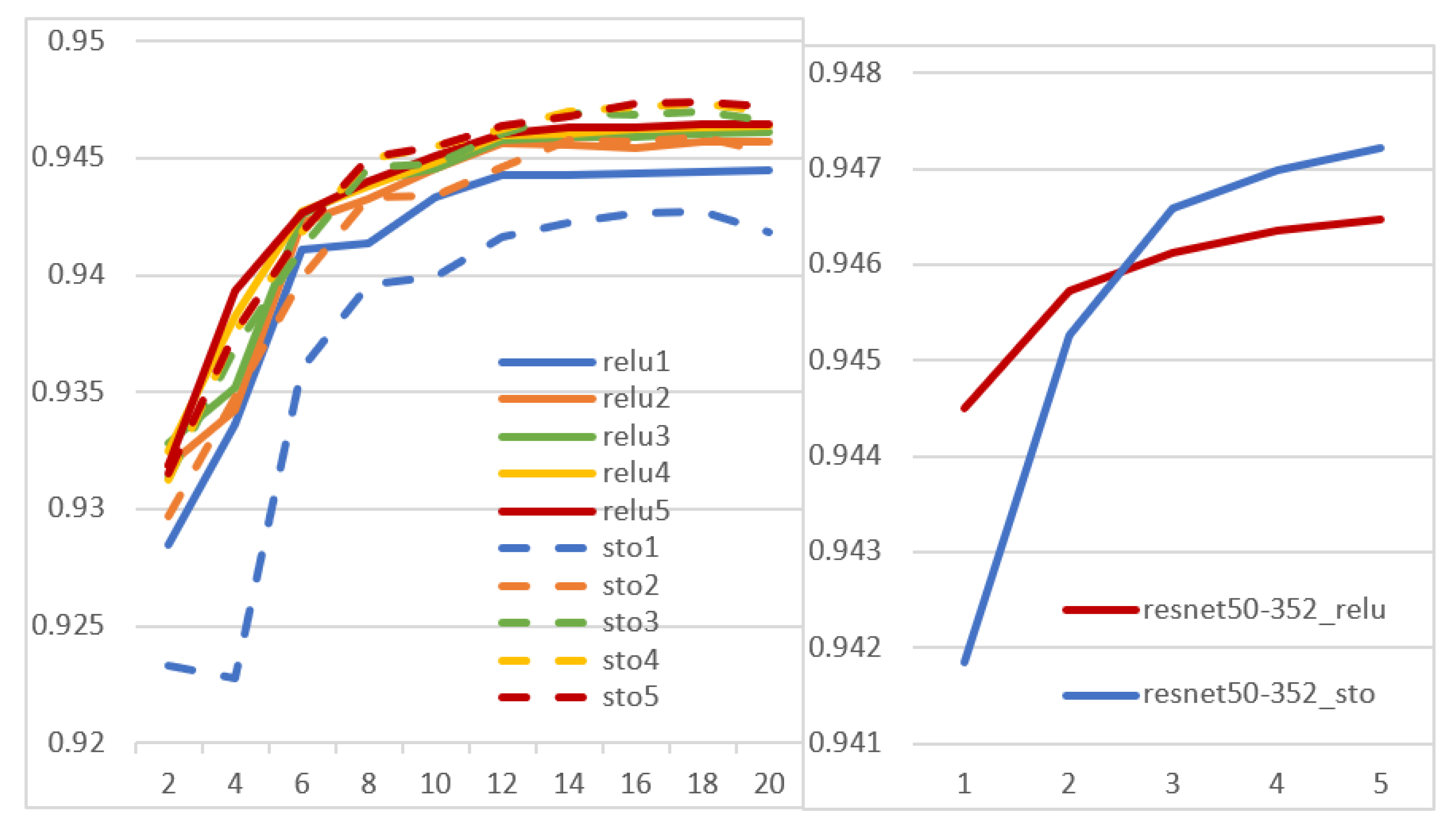
As a final experiment, we studied the performance of ensemble methods by varying the number of networks in the ensemble and the number of training epochs. For the sake of computation time, we considered only resnet50-352_relu vs. resnet50-352_sto, with the aim of studying the effects of stochastic activation selection in the design of ensembles. The graphs in Figure 2 report the performance obtained in the ECU testing set by ensembles of different sizes (each ensemble was obtained by adding a new network to the previous one, without any selection procedure). On the left, the performance of ensembles is reported as a function of the number of training epochs, and on the right, the performance at the final epoch is reported as a function of the number of networks. From both graphs, it is clear that even starting from a lower base performance (sto1 vs. relu1), the stochastic approach gains a higher advantage from the fusion. In the second graph, resnet50-352_sto outperforms resnet50-352_relu starting from Size 3.

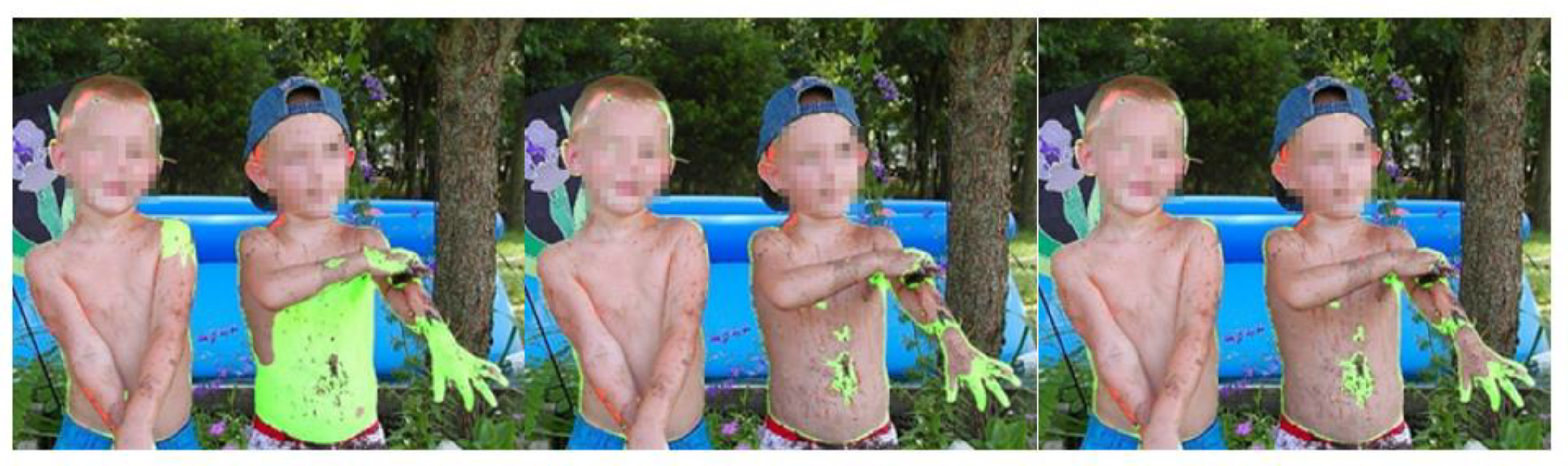
For a visive evaluation of improvements gained varying the size of an ensemble, some visualization results obtained by an ensemble of stochastic resnet50 composed of one, three, and five models are shown in Figure 3 (the image is from ECU).

5. Discussion

Clearly, using larger input sizes boosts the performance of Resnet50, as proved by results in Table 2 for standalone models and Table 3 for ensembles. For ensemble creation, stochastic variation of activation functions (sto) allows a performance improvement with respect to a simple fusion of network based on ReLu activations (relu) or a set of networks differing by the activation function (act). Moreover, the selection procedure (sel) allows for a further improvement. The best performance among the ensembles is obtained by resnet50-352_sel (Table 3).

Our best approach obtains the best performance, except for HarDNet-MSEG [23], a segmentation network based on weighted loss. Notice that our approach strongly outperforms several other deep learning approaches, including the recently published ColonSegNet [17] which works with a larger image size (512).

Of course, we are aware that ensemble methods greatly increase computational costs and complexity with respect to a standalone network. Regardless, since the networks in the ensemble are independent of each other, they can work in parallel. Furthermore, to reduce the computational effort of our approach, we suggest a simple rejection rule. Considering that in a real dataset, the incidence of images presenting polyps is quite low, we can use a first-level rule to reject images not containing polyps based on a single net, then use the ensemble only to gain a more precise segmentation if needed. Preliminary tests, using a very low threshold, suggest that it is possible to set a rule able to discard images not containing lesions without losing precision.

6. Conclusions

Semantic segmentation is a very important topic in medical image analysis and several other applications. In this paper, we aimed to propose and evaluate a novel approach for creating ensembles of CNNs by enhancing diversity among networks with different activation functions. The proposed approach was extensively evaluated on two very different segmentation problems, i.e., polyp segmentation during colonoscopy examinations and skin detection, gaining excellent results.

We compared several convolution neural network architectures, including ResNet, Xception, EfficentNet, MobileNet, HarDNet, and different methods for building ensembles of CNN.

Our reported results show that our best ensemble obtains state-of-the-art performance in both problems (Kvasir-SEG dataset, skin test sets), without ad hoc parameter optimization. To reproduce our results, the MATLAB source code is available at GitHub: https://github.com/LorisNanni (accessed on 5 nov. 2021).

In future work, we plan to deal with the complexity problem of deep neural networks. Deploying large models or big ensembles on the edge is infeasible, since smartphones and IoT sensors are resource-constrained devices; hence, it is vital to focus research also on techniques for compressing large models into a compact one with minimal performance loss. We plan to study the feasibility of reducing the complexity of our ensemble by applying one or more of the following techniques: pruning, quantization, low-rank factorization, and distillation.

References

- Feng, D.; Haase-Schütz, C.; Rosenbaum, L.; Hertlein, H.; Glaeser, C.; Timm, F.; Wiesbeck, W.; Dietmayer, K. Deep multi-modal object detection and semantic segmentation for autonomous driving: Datasets, methods, and challenges. IEEE Trans. Intell. Transp. Syst. 2020, 22, 1341–1360. [Google Scholar] [CrossRef] [Green Version]
- Brandao, P.; Zisimopoulos, O.; Mazomenos, E.; Ciuti, G.; Bernal, J.; Visentini-Scarzanella, M.; Menciassi, A.; Dario, P.; Koulaouzidis, A.; Arezzo, A.; et al. Towards a computed-aided diagnosis system in colonoscopy: Automatic polyp segmentation using convolution neural networks. J. Med. Robot. Res. 2018, 3, 1840002. [Google Scholar] [CrossRef] [Green Version]
- Noh, H.; Hong, S.; Han, B. Learning deconvolution network for semantic segmentation. In Proceedings of the IEEE International Conference on Computer Vision, Santiago, Chile, 7–13 December 2015; pp. 1520–1528. [Google Scholar]
- Badrinarayanan, V.; Kendall, A.; Cipolla, R. SegNet: A Deep Convolutional Encoder-Decoder Architecture for Image Segmentation. IEEE Trans. Pattern Anal. Mach. Intell. 2017, 39, 2481–2495. [Google Scholar] [CrossRef] [PubMed]
- Bullock, J.; Cuesta-Lázaro, C.; Quera-Bofarull, A. XNet: A convolutional neural network (CNN) implementation for medical X-Ray image segmentation suitable for small datasets. In Proceedings of the Medical Imaging 2019: Biomedical Applications in Molecular, Structural, and Functional Imaging, San Diego, CA, USA, 15 March 2019; Volume 10953, p. 109531Z. [Google Scholar]
- Shelhamer, E.; Long, J.; Darrell, T. Fully Convolutional Networks for Semantic Segmentation. IEEE Trans. Pattern Anal. Mach. Intell. 2017. [Google Scholar] [CrossRef]
- Roncucci, L.; Mariani, F. Prevention of colorectal cancer: How many tools do we have in our basket? Eur. J. Intern. Med. 2015, 26, 752–756. [Google Scholar] [CrossRef]
- Rein-Lien, H.; Abdel-Mottaleb, M.; Jain, A.K. Face detection in color images. IEEE Trans. Pattern Anal. Mach. Intell. 2002, 24, 696–706. [Google Scholar] [CrossRef] [Green Version]
- Argyros, A.A.; Lourakis, M.I.A. Real-time tracking of multiple skin-colored objects with a possibly moving camera. In European Conference on Computer Vision; Springer: Berlin/Heidelberg, Germany, 2004; pp. 368–379. [Google Scholar] [CrossRef]
- Han, J.; Award, G.M.; Sutherland, A.; Wu, H. Automatic skin segmentation for gesture recognition combining region and support vector machine active learning. In Proceedings of the 7th International Conference on Automatic Face and Gesture Recognition, Southampton, UK, 10–12 April 2006; pp. 237–242. [Google Scholar]
- Wang, Y.; Tavanapong, W.; Wong, J.; Oh, J.; De Groen, P.C. Part-based multiderivative edge cross-sectional profiles for polyp detection in colonoscopy. IEEE J. Biomed. Health Inform. 2013, 18, 1379–1389. [Google Scholar] [CrossRef]
- Mori, Y.; Kudo, S.; Berzin, T.M.; Misawa, M.; Takeda, K. Computer-aided diagnosis for colonoscopy. Endoscopy 2017, 49, 813. [Google Scholar] [CrossRef] [Green Version]
- Wang, P.; Xiao, X.; Brown, J.R.G.; Berzin, T.M.; Tu, M.; Xiong, F.; Hu, X.; Liu, P.; Song, Y.; Zhang, D.; et al. Development and validation of a deep-learning algorithm for the detection of polyps during colonoscopy. Nat. Biomed. Eng. 2018, 2, 741–748. [Google Scholar] [CrossRef]
- Thambawita, V.; Jha, D.; Riegler, M.; Halvorsen, P.; Hammer, H.L.; Johansen, H.D.; Johansen, D. The medico-task 2018: Disease detection in the gastrointestinal tract using global features and deep learning. arXiv 2018, arXiv:1810.13278. [Google Scholar]
- Guo, Y.B.; Matuszewski, B. Giana polyp segmentation with fully convolutional dilation neural networks. In Proceedings of the 14th International Joint Conference on Computer Vision, Imaging and Computer Graphics Theory and Applications, Prague, Czech Republic, 25–27 February 2019; pp. 632–641. [Google Scholar]
- Jha, D.; Smedsrud, P.H.; Riegler, M.A.; Halvorsen, P.; de Lange, T.; Johansen, D.; Johansen, H.D. Kvasir-SEG: A Segmented Polyp Dataset. In Proceedings of the 26th International Conference on Multimedia Modeling, Daejeon, Korea, 5–8 January 2020. [Google Scholar]
- Jha, D.; Ali, S.; Johansen, H.D.; Johansen, D.; Rittscher, J.; Riegler, M.A.; Halvorsen, P. Real-time polyp detection, localisation and segmentation in colonoscopy using deep learning. IEEE Access 2021, 9, 40496–40510. [Google Scholar] [CrossRef] [PubMed]
- Phung, S.L.; Bouzerdoum, A.; Chai, D. Skin segmentation using color pixel classification: Analysis and comparison. IEEE Trans. Pattern Anal. Mach. Intell. 2005, 27, 148–154. [Google Scholar] [CrossRef] [PubMed] [Green Version]
- Roy, K.; Mohanty, A.; Sahay, R.R. Deep Learning Based Hand Detection in Cluttered Environment Using Skin Segmentation. In Proceedings of the IEEE International Conference on Computer Vision Workshops (ICCVW), Venice, Italy, 22–29 October 2017; pp. 640–649. [Google Scholar]
- Arsalan, M.; Kim, D.S.; Owais, M.; Park, K.R. OR-Skip-Net: Outer residual skip network for skin segmentation in non-ideal situations. Expert Syst. Appl. 2020, 141, 112922. [Google Scholar] [CrossRef]
- Shahriar, S.; Siddiquee, A.; Islam, T.; Ghosh, A.; Chakraborty, R.; Khan, A.I.; Shahnaz, C.; Fattah, S.A. Real-time american sign language recognition using skin segmentation and image category classification with convolutional neural network and deep learning. In Proceedings of the TENCON 2018-2018 IEEE Region 10 Conference, Jeju, Korea, 28–31 October 2018; pp. 1168–1171. [Google Scholar]
- Lumini, A.; Nanni, L. Fair comparison of skin detection approaches on publicly available datasets. Expert Syst. Appl. 2020, 160, 113677. [Google Scholar] [CrossRef]
- Huang, C.-H.; Wu, H.-Y.; Lin, Y.-L. HarDNet-MSEG: A Simple Encoder-Decoder Polyp Segmentation Neural Network that Achieves over 0.9 Mean Dice and 86 FPS. arXiv 2021, arXiv:2101.07172. [Google Scholar]
- Ronneberger, O.; Fischer, P.; Brox, T. U-net: Convolutional networks for biomedical image segmentation. In Proceedings of the Medical Image Computing and Computer-Assisted Intervention—MICCAI 2015, Munich, Germany, 5–9 October 2015. [Google Scholar]
- Simonyan, K.; Zisserman, A. Very Deep Convolutional Networks for Large-Scale Image Recognition. Int. Conf. Learn. Represent. 2015, 1–14. [Google Scholar] [CrossRef] [Green Version]
- Chen, L.C.; Papandreou, G.; Kokkinos, I.; Murphy, K.; Yuille, A.L. DeepLab: Semantic Image Segmentation with Deep Convolutional Nets, Atrous Convolution, and Fully Connected CRFs. IEEE Trans. Pattern Anal. Mach. Intell. 2018, 40, 834–848. [Google Scholar] [CrossRef]
- Chen, L.C.; Zhu, Y.; Papandreou, G.; Schroff, F.; Adam, H. Encoder-decoder with atrous separable convolution for semantic image segmentation. In Proceedings of the 15th European Conference in Computer Vision, Munich, Germany, 8–14 September 2018. [Google Scholar]
- Minaee, S.; Boykov, Y.; Porikli, F.; Plaza, A.; Kehtarnavaz, N.; Terzopoulos, D. Image segmentation using deep learning: A Survey. IEEE Trans. Pattern Anal. Mach. Intelli. 2021. [Google Scholar] [CrossRef]
- Khan, A.; Sohail, A.; Zahoora, U.; Qureshi, A.S. A Survey of the Recent Architectures of Deep Convolutional Neural Networks. Artif. Intell. Rev. 2020, 53, 5455–5516. [Google Scholar] [CrossRef] [Green Version]
- Sandler, M.; Howard, A.; Zhu, M.; Zhmoginov, A.; Chen, L.C. MobileNetV2: Inverted Residuals and Linear Bottlenecks. In Proceedings of the IEEE Computer Society Conference on Computer Vision and Pattern Recognition, Salt Lake City, UT, USA, 18–22 June 2018. [Google Scholar]
- He, K.; Zhang, X.; Ren, S.; Sun, J. Deep Residual Learning for Image Recognition. In Proceedings of the 2016 IEEE Conference on Computer Vision and Pattern Recognition (CVPR), Las Vegas, NV, USA, 27–30 June 2016; pp. 770–778. [Google Scholar]
- Chollet, F. Xception: Deep learning with depthwise separable convolutions. In Proceedings of the 30th IEEE Conference on Computer Vision and Pattern Recognition, Honolulu, HI, USA, 21–26 July 2017. [Google Scholar]
- Szegedy, C.; Ioffe, S.; Vanhoucke, V.; Alemi, A.A. Inception-v4, Inception-ResNet and the Impact of Residual Connections on Learning. Proc. IEEE Int. Conf. Comput. Vis. 2017, 115, 4278–4284. [Google Scholar] [CrossRef] [Green Version]
- Tan, M.; Le, Q.V. EfficientNet: Rethinking model scaling for convolutional neural networks. In Proceedings of the 36th International Conference on Machine Learning, Long Beach, CA, USA, 9–15 June 2019. [Google Scholar]
- Sudre, C.H.; Li, W.; Vercauteren, T.; Ourselin, S.; Jorge Cardoso, M. Generalised dice overlap as a deep learning loss function for highly unbalanced segmentations. In Deep Learning in Medical Image Analysis and Multimodal Learning for Clinical Decision Support; Springer: Cham, Switzerland, 2017. [Google Scholar] [CrossRef] [Green Version]
- Jadon, S. A survey of loss functions for semantic segmentation. In Proceedings of the 2020 IEEE Conference on Computational Intelligence in Bioinformatics and Computational Biology, Viña del Mar, Chile, 27–29 October 2020. [Google Scholar]
- Nanni, L.; Lumini, A.; Ghidoni, S.; Maguolo, G. Stochastic selection of activation layers for convolutional neural networks. Sensors 2020, 20, 1626. [Google Scholar] [CrossRef] [PubMed] [Green Version]
- Glorot, X.; Bordes, A.; Bengio, Y. Deep sparse rectifier neural networks. In Proceedings of the 14th International Conference on Artificial Intelligence and Statistics (AISTATS) 2011, Fort Lauderdale, FL, USA, 26–29 August 2011. [Google Scholar]
- Maas, A.L.; Hannun, A.Y.; Ng, A.Y. Rectifier nonlinearities improve neural network acoustic models. In Proceedings of the in ICML Workshop on Deep Learning for Audio, Speech and Language Processing, Atlanta, GA, USA, 16 June 2013. [Google Scholar]
- Clevert, D.A.; Unterthiner, T.; Hochreiter, S. Fast and accurate deep network learning by exponential linear units (ELUs). In Proceedings of the 4th International Conference on Learning Representations, San Juan, Puerto Rico, 2–4 May 2016. [Google Scholar]
- He, K.; Zhang, X.; Ren, S.; Sun, J. Delving deep into rectifiers: Surpassing human-level performance on imagenet classification. In Proceedings of the IEEE International Conference on Computer Vision, Santiago, Chile, 7–13 December 2015. [Google Scholar]
- Jin, X.; Xu, C.; Feng, J.; Wei, Y.; Xiong, J.; Yan, S. Deep learning with S-shaped rectified linear activation units. In Proceedings of the 30th AAAI Conference on Artificial Intelligence, Phoenix, AZ, USA, 12–17 February 2016. [Google Scholar]
- Agostinelli, F.; Hoffman, M.; Sadowski, P.; Baldi, P. Learning activation functions to improve deep neural networks. In Proceedings of the 3rd International Conference on Learning Representations, San Diego, CA, USA, 7–9 May 2015. [Google Scholar]
- Maguolo, G.; Nanni, L.; Ghidoni, S. Ensemble of Convolutional Neural Networks Trained with Different Activation Functions. Expert Syst. Appl. 2021, 166, 114048. [Google Scholar] [CrossRef]
- Cheng, Q.; Li, H.; Wu, Q.; Ma, L.; King, N.N. Parametric Deformable Exponential Linear Units for deep neural networks. Neural Netw. 2020, 125, 281–289. [Google Scholar] [CrossRef] [PubMed]
- Ramachandran, P.; Zoph, B.; Le, Q. V Searching for Activation Functions. arXiv 2017, arXiv:1710.05941. [Google Scholar]
- Zhou, Y.; Li, D.; Huo, S.; Kung, S.-Y. Soft-Root-Sign Activation Function. arXiv 2020, arXiv:2003.00547. [Google Scholar]
- Misra, D. Mish: A self regularized non-monotonic neural activation function. arXiv 2019, arXiv:1908.08681. [Google Scholar]
- Pudil, P.; Novovičová, J.; Kittler, J. Floating search methods in feature selection. Pattern Recognit. Lett. 1994, 15, 1119–1125. [Google Scholar] [CrossRef]
- Safarov, S.; Whangbo, T.K. A-denseunet: Adaptive densely connected unet for polyp segmentation in colonoscopy images with atrous convolution. Sensors 2021, 21, 1441. [Google Scholar] [CrossRef]
- Branch, M.V.L.; Carvalho, A.S. Polyp Segmentation in Colonoscopy Images using U-Net-MobileNetV2. arXiv 2021, arXiv:2103.15715. [Google Scholar]
- Tomar, N.K.; Jha, D.; Ali, S.; Johansen, H.D.; Johansen, D.; Riegler, M.A.; Halvorsen, P. DDANet: Dual Decoder Attention Network for Automatic Polyp Segmentation. In International Conference on Pattern Recognition; Springer: Cham, Switzerland, 2021; ISBN 9783030687922. [Google Scholar]
- Stöttinger, J.; Hanbury, A.; Liensberger, C.; Khan, R. Skin paths for contextual flagging adult videos. In Advances in Visual Computing; Springer: Berlin/Heidelberg, Germany, 2009. [Google Scholar] [CrossRef]
- Tan, W.R.; Chan, C.S.; Yogarajah, P.; Condell, J. A Fusion Approach for Efficient Human Skin Detection. Ind. Inf. IEEE Trans. 2012, 8, 138–147. [Google Scholar] [CrossRef] [Green Version]
- Huang, L.; Xia, T.; Zhang, Y.; Lin, S. Human skin detection in images by MSER analysis. In Proceedings of the 2011 18th IEEE International Conference on Image Processing, Brussels, Belgium, 11–14 September 2011; pp. 1257–1260. [Google Scholar] [CrossRef]
- Ruiz-Del-Solar, J.; Verschae, R. Skin detection using neighborhood information. In Proceedings of the Proceedings—Sixth IEEE International Conference on Automatic Face and Gesture Recognition, Seoul, Korea, 17–19 May 2004; pp. 463–468. [Google Scholar]
- Jones, M.J.; Rehg, J.M. Statistical color models with application to skin detection. Int. J. Comput. Vis. 2002, 46, 81–96. [Google Scholar] [CrossRef]
- Casati, J.P.B.; Moraes, D.R.; Rodrigues, E.L.L. SFA: A human skin image database based on FERET and AR facial images. In Proceedings of the IX Workshop de Visao Computational, Rio de Janeiro, Brazil, 30 January–1 February 2013. [Google Scholar]
- Kawulok, M.; Kawulok, J.; Nalepa, J.; Smolka, B. Self-adaptive algorithm for segmenting skin regions. EURASIP J. Adv. Signal Process. 2014, 2014, 1–22. [Google Scholar] [CrossRef] [Green Version]
- Schmugge, S.J.; Jayaram, S.; Shin, M.C.; Tsap, L.V. Objective evaluation of approaches of skin detection using ROC analysis. Comput. Vis. Image Underst. 2007, 108, 41–51. [Google Scholar] [CrossRef]
- Sanmiguel, J.C.; Suja, S. Skin detection by dual maximization of detectors agreement for video monitoring. Pattern Recognit. Lett. 2013, 34, 2102–2109. [Google Scholar] [CrossRef] [Green Version]
- Abdallah, A.S.; El-Nasr, M.A.; Abbott, A.L. A new color image database for benchmarking of automatic face detection and human skin segmentation techniques. World Academy of Science, Engineering and Technology, Open Science Index 12. Int. J. Comput. Inf. Eng. 2007, 1, 3782–3786. [Google Scholar]
Figure 1.
Pseudocode of the procedures for stochastic activation selection.
Figure 2.
Performance on the ECU testing set (F1-score): on the left, performance as a function of the training epochs for ensembles of size varying from 1 to 5. On the right is the performance as a function of the ensemble size.
Figure 3.
Visualization results with the model resnet50-352_sto by varying its size. Green indicates missed skin, and red is the wrong prediction.