
Double-Talk Detection-Aided Residual Echo Suppression via Spectrogram Masking and Refinement


Andrew and Erna Viterbi Faculty of Electrical & Computer Engineering, Technion–Israel Institute of Technology, Technion City, Haifa 3200003, Israel
*
Authors to whom correspondence should be addressed.
Acoustics 2022, 4(3), 637-655; https://doi.org/10.3390/acoustics4030039
Submission received: 10 July 2022
/
Revised: 21 August 2022
/
Accepted: 23 August 2022
/
Published: 25 August 2022
(This article belongs to the Special Issue Acoustics, Speech and Signal Processing)
Abstract
:Acoustic echo in full-duplex telecommunication systems is a common problem that may cause desired-speech quality degradation during double-talk periods. This problem is especially challenging in low signal-to-echo ratio (SER) scenarios, such as hands-free conversations over mobile phones when the loudspeaker volume is high. This paper proposes a two-stage deep-learning approach to residual echo suppression focused on the low SER scenario. The first stage consists of a speech spectrogram masking model integrated with a double-talk detector (DTD). The second stage consists of a spectrogram refinement model optimized for speech quality by minimizing a perceptual evaluation of speech quality (PESQ) related loss function. The proposed integration of DTD with the masking model outperforms several other configurations based on previous studies. We conduct an ablation study that shows the contribution of each part of the proposed system. We evaluate the proposed system in several SERs and demonstrate its efficiency in the challenging setting of a very low SER. Finally, the proposed approach outperforms competing methods in several residual echo suppression metrics. We conclude that the proposed system is well-suited for the task of low SER residual echo suppression.
1. Introduction
Modern telecommunication systems often suffer from speech intelligibility degradation caused by an acoustic echo. A typical scenario includes two speakers communicating between a far-end and a near-end point. At the near-end point, a microphone captures both the near-end speaker’s signal and the acoustic echo of a loudspeaker playing the far-end signal [1]. When the far-end speaker speaks, he hears the echo of his voice, thus reducing the quality of the conversation. Therefore, canceling the acoustic echo while preserving near-end speech quality is desired in any full-duplex communication system. Linear acoustic echo cancellers (AECs) are commonly employed to cancel the echo component of the microphone signal and are traditionally based on linear adaptive filters [2]. Linear AECs estimate the acoustic path from the loudspeaker to the microphone. The estimated filters are applied to the far-end reference signal resulting in an estimate of the echo signal as received by the microphone. Then, the estimated near-end signal is obtained by subtracting the estimated echo from the microphone signal. However, due to their linear nature, residual non-linear components of the echo remain at the output of the linear AECs. In most cases, the residual echo still interferes and degrades the near-end speech quality.
In recent years, deep-learning neural networks (DNNs) achieved unprecedented performance in many fields, e.g., computer vision, natural language processing, audio and speech processing, and more. Possessing high non-linear modeling capabilities, DNNs became a natural choice for acoustic echo cancellation. Zhang and Wang [3] employ a bi-directional long short-term memory (BLSTM) [4] recurrent neural network (RNN) operating in the time-frequency (T-F) domain to capture dependency between time frames. The model predicts an ideal ratio mask (IRM) [5] applied to the microphone signal’s spectrogram magnitudes to estimate the near-end signal’s spectrogram magnitudes. Kim and Chang [6] propose a time-domain U-Net [7] architecture with an additional encoder that learns features from the far-end reference signal. An attention mechanism [8] accentuates the meaningful far-end features for the U-Net’s encoder. Westhausen and Meyer [9] combine T-F and time-domain processing by adapting the dual-signal transformation LSTM network (DTLN) [10] to the task of acoustic echo cancellation. Although DNN AECs achieve performance superior to linear AECs and allow for end-to-end training and inference, they are prone to introducing distortion to the estimated near-end signal, especially when the signal-to-echo ratio (SER) is low.
An alternative for end-to-end DNN acoustic echo cancellation is residual echo suppression. In a typical residual echo suppression setting, a linear AEC is followed by a DNN aimed at suppressing the residual echo at the output of the linear AEC. Linear AECs introduce little distortion to the near-end signal. Their estimation of the echo and near-end signals provides the residual echo suppressor (RES) with better features, allowing for better near-end estimation with smaller model sizes. Carbajal et al. [11] propose a simple fully-connected architecture that receives the spectrogram magnitudes of the far-end reference signal and the linear AEC’s outputs and predicts a phase-sensitive filter (PSF) [12] to recover the near-end signal from the linear AEC’s error signal. Pfeifenberger and Pernkopf [13] suggest utilizing an LSTM to predict a T-F gain mask from the log differences between the powers of the microphone signal and the AEC’s echo estimate. Chen et al. [14] propose a time-domain RES based on the well-known Conv-TasNet architecture [15]. They employ a multi-stream modification of the original architecture, where the outputs of the linear AEC are separately encoded before being fed to the main Conv-TasNet. Fazel et al. [16] propose context-aware deep acoustic echo cancellation (CAD-AEC), which incorporates a contextual attention module to predict the near-end signal’s spectrogram magnitudes from the microphone and linear AEC output signals. Halimeh et al. [17] employ a complex-valued convolutional recurrent network (CRN) to estimate a complex T-F mask applied to the complex spectrogram of the AEC’s error signal to recover the near-end signal’s spectrogram. Ivry et al. [18] employ a 2-D U-Net operating on the spectrogram magnitudes of the linear AEC’s outputs. A custom loss function with a tunable parameter allows a dynamic tradeoff between the levels of echo suppression and estimated signal distortion. Franzen and Fingscheidt [19] propose a 1-D fully convolutional recurrent network (FCRN) operating on discrete Fourier transform (DFT) inputs. An ablation study is performed to study the effect of different combinations of input signals on the joint task of residual echo suppression and noise reduction. Although achieving state-of-the-art residual echo suppression performance, none of the above studies focus on the challenging scenario of extremely low SER. Low SER may occur in typical real-life situations such as a conversation over a mobile phone where the loudspeaker plays the echo at a high volume.
In a typical residual echo suppression scenario, one of four situations may occur at each time point: both speakers are silent, only the far-end speaker speaks, only the near-end speaker speaks, and double-talk, where both speakers speak at the same time. When only the near-end speaker speaks, the microphone signal should remain unchanged to keep the near-end speech distortionless. Ideally, the microphone signal should be canceled when only far-end speech is present to remove any echo component. The challenging situation is double-talk, where it is desired to cancel the echo of the far-end speech while keeping the near-end speech distortion to a minimum. Therefore, it is natural to integrate a double-talk detector (DTD) into the system. Linear AECs typically employ a DTD to prevent the cancellation of the near-end speech in double-talk situations [20,21]. Several studies also integrate double-talk detection in deep-learning acoustic echo cancellation or residual echo suppression models. Zhang et al. [22] employ an LSTM, which operates on the spectrogram magnitudes of the microphone and far-end reference signals, and predicts near-end speech presence via a binary mask that is applied to the output of the DNN AEC. Zhou and Leng [23] formulate the problem as a multi-task learning problem where a single DNN learns to perform residual echo suppression and double-talk detection in tandem. The model consists of two output branches: the first branch predicts a PSF and acts as a RES and the second branch detects double-talk. The RES is conditioned on the DTD’s predictions by supplying it with features before the classification. Ma et al. [24] propose to perform double-talk detection with two voice activity detectors (VADs), one for detecting near-end speech and the other for detecting far-end speech. Features from several layers of the VADs are fed to a gated recurrent unit (GRU) [25] RNN that performs residual echo suppression. Ma et al. [26] propose a multi-class classifier that receives the encoded features of the time-domain microphone and far-end signals and classifies each time frame independently of the AEC’s predictions. Zhang et al. [27] also incorporate a VAD as an independent output branch in a residual echo suppression model. While exhibiting high residual echo performance, their results show that adding the VAD does not lead to improved objective metrics. The rest of the works mentioned above do not study the effect of the DTD/VAD on the RES’s performance. Therefore, it is worth studying the effect of DTD and RES integration configurations on the system’s performance, especially in the low SER setting where the echo may entirely screen the near-end speech.
This study proposes a two-stage residual echo suppression deep-learning system focused on the challenging low SER scenario. Our approach is inspired by [28], where a two-stage spectrogram masking and inpainting approach is taken to tackle the low signal-to-noise ratio (SNR) speech enhancement problem. We adopt this approach to the residual echo suppression setting while introducing changes and improvements. The first stage in our system is double-talk detection and spectrogram masking. We propose an architecture with fewer parameters and a faster inference time than the masking stage in [28]. Furthermore, we study several ways of integrating double-talk detection in our model based on previous studies and show that the proposed configuration achieves the most significant improvement in residual echo suppression performance. The second stage in our system is spectrogram refinement. Unlike [28], where the second stage consists of creating holes in the spectrogram and applying spectrogram inpainting to reconstruct the desired signal, we propose instead to perform spectrogram refinement. We optimize the model to maximize the desired speech quality measured by the perceptual evaluation of speech quality (PESQ) [29] score by minimizing the perceptual metric for speech quality evaluation (PMSQE) loss function [30]. We perform an ablation study to show the effectiveness of every component of the proposed system. Furthermore, we train and evaluate the proposed system in several levels of SER and show that it is most effective in the extremely-low SER setting. Finally, we compare the proposed system to several other residual echo suppression systems and show that it outperforms others in several residual echo suppression and speech quality measures.
2. Materials and Methods
In this section, we first formulate the problem of residual echo suppression and denote the different signals. Next, we present the various components of the proposed system. Lastly, we discuss the data used for training and evaluation and provide details about the training procedures.
2.1. Problem Formulation
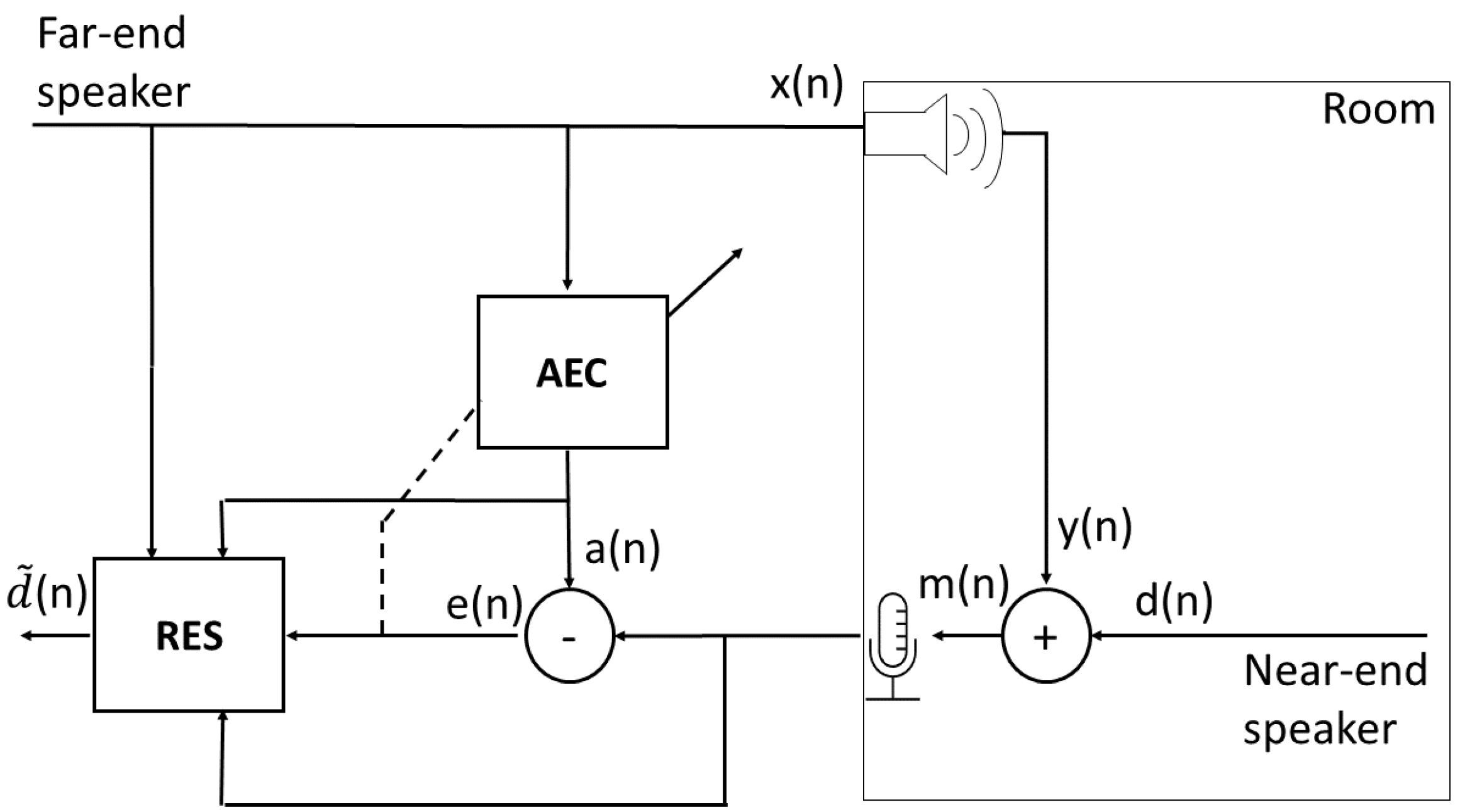
To formulate the problem of residual echo suppression, we denote the different signals as follows: denotes the far-end reference signal at time point n. We denote the echoic loudspeaker signal received by the microphone by and the near-end speaker’s signal by . The microphone signal is denoted by and is given by
The inputs to the linear AEC are and , and its outputs are and , the estimated echo signal and the error signal, respectively. The goal is to enhance to obtain a better estimate of by further suppressing the residual echo. denotes the estimated near-end speaker’s signal at the entire system’s output. Figure 1 depicts the residual echo suppression setup and the different signals. The following sections will refer to the spectrogram magnitudes of the different signals’ short-time Fourier transform (STFT). These will be denoted by capital letters of their respective time-domain signal notation, e.g., is the STFT spectrogram magnitude of , where f and k denote the frequency-bin and time-bin indices, respectively.
2.2. Proposed System
The proposed system comprises three modules: A linear AEC, a double-talk detection and spectrogram masking model, and a spectrogram refinement model. The masking and spectrogram refinement models together form the RES. They are inspired by [28], where a two-stage deep-learning system consisting of spectrogram masking and spectrogram inpainting performs speech enhancement. To better suit the task of residual echo suppression, we present a few changes and improvements, as will be detailed in the following sub-sections.
2.2.1. Linear Acoustic Echo Cancellation
We employ an AEC with the normalized sign-error least mean squares (NSLMS) [31] algorithm for linear acoustic echo cancellation. NSLMS adjusts each filter tap’s weight according to the error signal’s sign. Despite the NSLMS being less common for acoustic echo cancellation than the normalized least mean squares (NLMS), several studies have shown its advantages over the NLMS [32,33]. We employ a subband domain NSLMS that transforms the signals using uniform single-sideband filter banks [34]. Each subband’s filter tap weights are updated according to the update equation
In the above equation, is the step size. The vector is the filter tap weights vector, N is the number of filter taps, and is the transpose operation. The vector is the far-end reference signal vector of length N at time n, and is the signum function. The normalization factor allows the steady-state error of the AEC to be independent of the far-end signal’s power [35].
2.2.2. Double-Talk Detection and Spectrogram Masking
The spectrogram masking model aims to perform a significant portion of the residual echo suppression. The greatest challenge in residual echo suppression is suppressing the echo during double-talk periods while reducing the near-end speech distortion. Therefore, the model may benefit from optimization for double-talk detection in tandem with residual echo suppression.
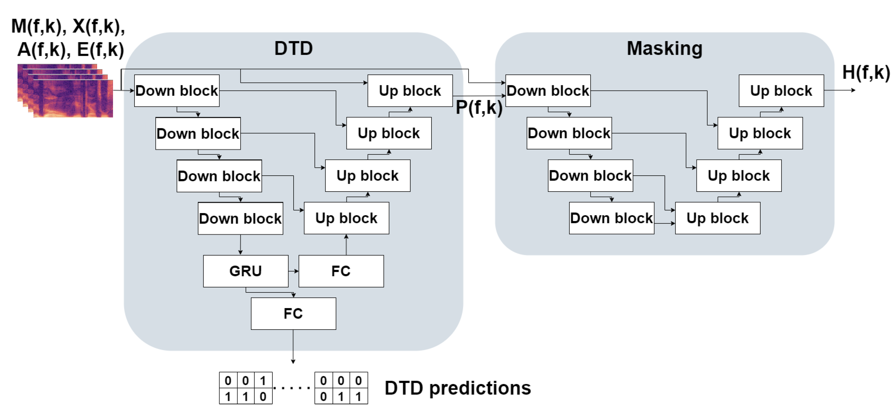
In the masking stage, we employ the U-Net architecture [7]. This architecture differs from the one in [28], where the architecture comprises convolutional blocks consisting of residual connections, requiring more model parameters and resulting in a longer inference time than the U-Net architecture while achieving similar performance. U-Net has a fully-convolutional encoder-decoder structure with skip connections between levels of the encoder and the decoder. The proposed model is a concatenation of two U-Nets. The first U-Net performs double-talk detection and is also used to learn a feature representation from the double-talk predictions and the input signals used for the masking task. The second U-Net receives the outputs of the first U-Net and all input signals and predicts a spectrogram ratio mask.
The first U-Net’s input is the log of the input signals , , , and , concatenated along the channel dimension. The encoder comprises down-sampling convolution blocks (referred to as “down-blocks” from here on), where each block consists of a 2-D convolution layer, instance normalization layer [36], and leaky rectified linear unit (leaky ReLU) [37] activation function. The convolution window stride is 2 along the frequency dimension and 1 along the time dimension—effectively down-sampling the inputs along the frequency dimension while preserving the time dimension. The output of the encoder is fed to a uni-directional GRU which learns time dependency between the different frames. The GRU’s output has two purposes—it is used both as features utilized by a classifier that predicts double-talk for each time frame and as inputs to the decoder, which learns a representation from the DTD’s features. We frame the double-talk detection task as a binary multi-label classification task, where each time frame is labeled as either containing near-end speech or not as well as either containing far-end speech or not. We empirically found that this approach leads to better classification performance than the more common approach of multi-class classification, where each time frame is assigned a single label (most commonly, the labels are: silence, near-end speech only, far-end speech only, or double-talk). In order to classify each time frame, the outputs of the GRU are fed to a fully-connected layer responsible for reducing the feature dimension (while preserving the time dimension as we want to classify each time frame) to 2, which corresponds to the two possible labels.
The features learned by the encoder for double-talk detection are employed to assist the task of learning a spectrogram mask. Instead of directly feeding the masking U-Net with the encoder’s features, the decoder learns a feature representation. The decoder comprises up-blocks similar to down-blocks, except that the inputs are first up-sampled via nearest-neighbor up-sampling with a factor of 2 along the frequency dimension and 1 along the time dimension. The up-sampled inputs are concatenated along the channel dimension with the outputs of the matching level of the encoder. The output of the decoder, , has a single channel and is of the same frequency and time dimensions as the input signals. In order to learn a spectrogram mask, an additional U-Net is concatenated to the first U-Net. This U-Net accepts as inputs the log of all input signals , , , and , as well as the output of the first U-Net , resulting in 5 input channels. The second U-Net’s structure is similar to that of the first U-Net with a few exceptions - the down-sampling (as well as the up-sampling) factor is 2 for both frequency and time dimensions, and the last decoder block contains neither an activation function nor a normalization layer. The model’s output, denoted by , consists of one channel and has the same frequency and time dimensions as the input signals. The entire DTD and masking model’s architecture is depicted in Figure 2.
As previously mentioned, we empirically found that the DTD performs better when trained to detect near-end and far-end speech separately for each time frame. Therefore, the DTD’s training target for each utterance is a tensor of shape , where B is the batch size, and T is the number of time frames. The first and second rows of the second dimension represent the presence of near-end speech and far-end speech, respectively, where 1 indicates the presence of speech and 0 represents its absence. The training target of the masking model is the log of the ratio between the spectrogram magnitudes of the clean near-end speech and that of the error signal, denoted by and given by
where and are small constants for numerical stability. The loss function used for the double-talk detection task is denoted by and given by
where and are binary cross entropy (BCE) loss terms for near-end and far-end speech detection, respectively. The quantity is given by
where is the ground-truth label for time frame k, is the predicted label for time frame k, and is the sigmoid function. is similarly defined. For the masking task, we use the mean squared error (MSE) loss between the labels and the outputs, denoted by and given by
where n is the total number of spectrogram bins. The overall loss function used to optimize the model is a weighted sum of the two loss functions with a weight parameter applied to :
2.2.3. Spectrogram Refinement
The spectrogram masking approach alone may not be sufficient to both suppress the residual echo and preserve the near-end speech’s quality. It is especially true in the low SER scenario, where the echo signal’s energy is considerably higher than the near-end signal’s. In this case, spectrogram masking can suppress the residual echo to a large degree, at the cost of degrading the near-end speech quality. In the most severe cases, the masking operation completely cancels parts of the near-end speech during double-talk. In [28], following the masking stage, the speech is further enhanced by a spectrogram inpainting stage. The inpainting operation aims to reconstruct spectrogram bins containing speech canceled in the masking stage. In the residual echo suppression case, near-end speech is screened by the far-end echoic speech rather than noise. The screening renders the reconstruction operation more challenging as it may be difficult to distinguish the speech components of the near-end signal from those of the far-end signal. Instead, we frame this stage as spectrogram refinement, where the mask learned by the masking model is used as an additional feature along with the input signals rather than to mask the signal from which we want to obtain the desired near-end speech.
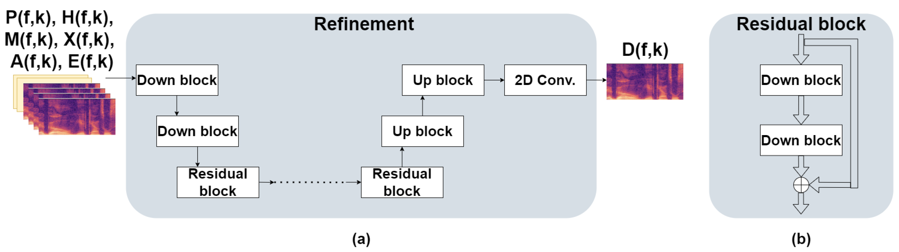
For spectrogram refinement, we adopt the architecture used in [28]. In our experiments, we found that when using the U-Net architecture for this stage, the model’s performance was almost identical to the performance of the masking model. Since the masking model achieves good performance on its own, and due to the skip connection between the inputs and the decoder outputs, the refinement model with the U-Net architecture achieved negligible performance gain compared to the masking model. Instead, we employ a fully-convolutional architecture consisting of residual connection blocks, as proposed in [28].
The input to the model is the log of the input signals , , , and , the output of the masking model , and the double-talk features , concatenated along the channel dimension. The input is first fed to two consecutive down-blocks similar to the encoder blocks in the masking stage. The inputs are down-sampled by a factor of 2 along both time and frequency dimensions. Instead of leaky ReLU, we employ an exponential linear unit (ELU) activation function [38] as proposed in [28]. Following the down-blocks is a series of identical residual blocks. A residual block comprises two consecutive down-blocks with a convolution kernel stride . The output of the second convolution block is summed element-wise with the input to the residual block. Following the last residual block are two up-blocks with an up-sampling factor of 2 along both time and frequency dimensions. The output layer is a 2-D convolution layer with one output channel. Figure 3 depicts the refinement model’s architecture and the residual blocks.
We frame the refinement stage as a regression task, where the model learns to predict the near-end spectrogram magnitudes directly. Therefore, the training target is the log of the near-end signal’s spectrogram magnitudes , where is a small constant for numerical stability. Inverting the log operation and applying inverse STFT (iSTFT) using the error signal’s phase, we obtain the time-domain near-end signal . Since a significant portion of the residual echo was suppressed in the masking stage, the main goal of the refinement stage is to improve the estimated near-end speech quality. We achieve this goal by optimizing the model for speech quality measured by PESQ. Since the PESQ function is non-differentiable, it cannot be used as a loss function in gradient-descent-based algorithms. The PMSQE loss function [30] aims to approximate PESQ with a differentiable function. PMSQE, unlike MSE, takes into account perceptual-related features of the predicted signal by incorporating two disturbance terms inspired by the PESQ algorithm. We denote the PMSQE loss term by (for brevity, we do not formulate the loss function and its different components here - the reader is referred to [30] for additional details). We empirically found that minimizing the PMSQE loss function alone does not achieve the desired results since, although the loss value converges, the different evaluation metrics diverge. Therefore, we add a regularizing MSE loss term defined as
The complete loss function minimized during the refinement model training is given by
where is a weight parameter. The specifications for each model are detailed in Appendix A. Code is provided in [39].
2.3. Datasets
We employ an independently recorded dataset to train and evaluate the proposed system in real-life conditions. Several conditions and configurations were considered when conducting the recordings. A total of h of speech from the TIMIT [40] corpus and h of speech from the LibriSpeech [41] corpus were used in the recordings. Recorded data were split between the training and test sets, such that the test set contains unique speakers not shared by the training set and unique conditions and setups not seen during training. In order to augment the training dataset, synthetic data from the ICASSP 2021 AEC challenge dataset [42] were also used during training. In of the cases, the far-end signal in the synthetic dataset was processed with a nonlinear function. Some examples of nonlinear functions are clipping of the maximum value, a sigmoidal function, or a learned nonlinear distortion function. More details regarding the synthetic data can be found in [42]. The SER in both datasets (synthetic and independent recordings) was set to dB. For analysis in different SERs, the same data were used in every experiment, where the SER was set to dB, dB, or dB. The combined dataset consists of h of data with a 16 kHz sampling rate. Further details regarding the data and training procedures can be found in Appendix B.
3. Results
This section presents the performance measures used to evaluate the different systems, shows the ablation study results, and compares the proposed system with two other systems. Audio examples of the proposed system’s output, along with the microphone, error, and clean near-end speech, can be found in [39].
3.1. Performance Measures
In order to evaluate the performance of the proposed and compared systems, two scenarios are considered: far-end only and double-talk. Near-end only periods are not considered for performance evaluation since all systems introduce little distortion to the input signal when no echo is present. Furthermore, since it is a trivial task to determine that the far-end speaker is silent, during these periods, the microphone signal can be directly passed to the system’s output. Thus, no distortion will be applied to it.
During far-end only periods, we expect the enhanced signal to have as low energy as possible (ideally, it is completely silent). Therefore, performance is evaluated during these periods using the echo return loss enhancement (ERLE), which measures the echo reduction between the microphone signal and the enhanced signal. ERLE is measured in dB and is defined as
ERLE may not always correlate well with human subjective ratings [43]. AEC mean opinion score (AECMOS) [44] provides a speech quality assessment metric for evaluating echo impairment that overcomes the drawbacks of conventional methods. AECMOS is a DNN trained to directly predict subjective ratings for echo impairment using ground-truth human ratings of more than 148 h of data. The model predicts two scores in the range , one for echo impairment (AECMOS-echo) and the other for other degradations (AECMOS-degradations). The model distinguishes between three scenarios: near-end single-talk, far-end single-talk, and double-talk. In the far-end single-talk case, only AECMOS-echo is considered.
We aim to suppress the residual echo during double-talk periods while maintaining the near-end speech’s quality. During these periods, performance is evaluated using two different measures. The first measure is perceptual evaluation of speech quality (PESQ) [29]. PESQ is an intrusive speech quality metric based on an algorithm designed to approximate a subjective evaluation of a degraded audio sample. PESQ score range is , where a higher score indicates better speech quality. However, like ERLE, PESQ does not always correlate well with subjective human ratings. Therefore, the second performance measure is AECMOS-echo which measures the echo reduction during double-talk periods. We do not use AECMOS-degradations for performance evaluation for two reasons. The first reason is that we focus on the low SER scenario without including intense noise or distortions, which may cause additional degradation. The second reason is that, as we show in the results, AECMOS-degradations fail to capture the true residual echo suppression performance in the low SER case.
Finally, although not a performance measure, we formally define SER, measured in double-talk periods and used to measure the near-end signal’s energy relative to the echo signal’s energy. SER is expressed in dB as
3.2. Ablation Study
First, we present the ablation study’s results, showing how each part of the proposed system contributes to the performance. Table 1 shows the performance of the AEC, the performance of the AEC followed by the masking stage with and without double-talk detection (AEC+M+D and AEC+M, respectively), the performance of the AEC followed by the refinement stage without the masking stage’s outputs (AEC+R, using only the input signals), and the entire system’s performance—AEC followed by masking and double-talk detection followed by the refinement model (AEC+M+D+R).
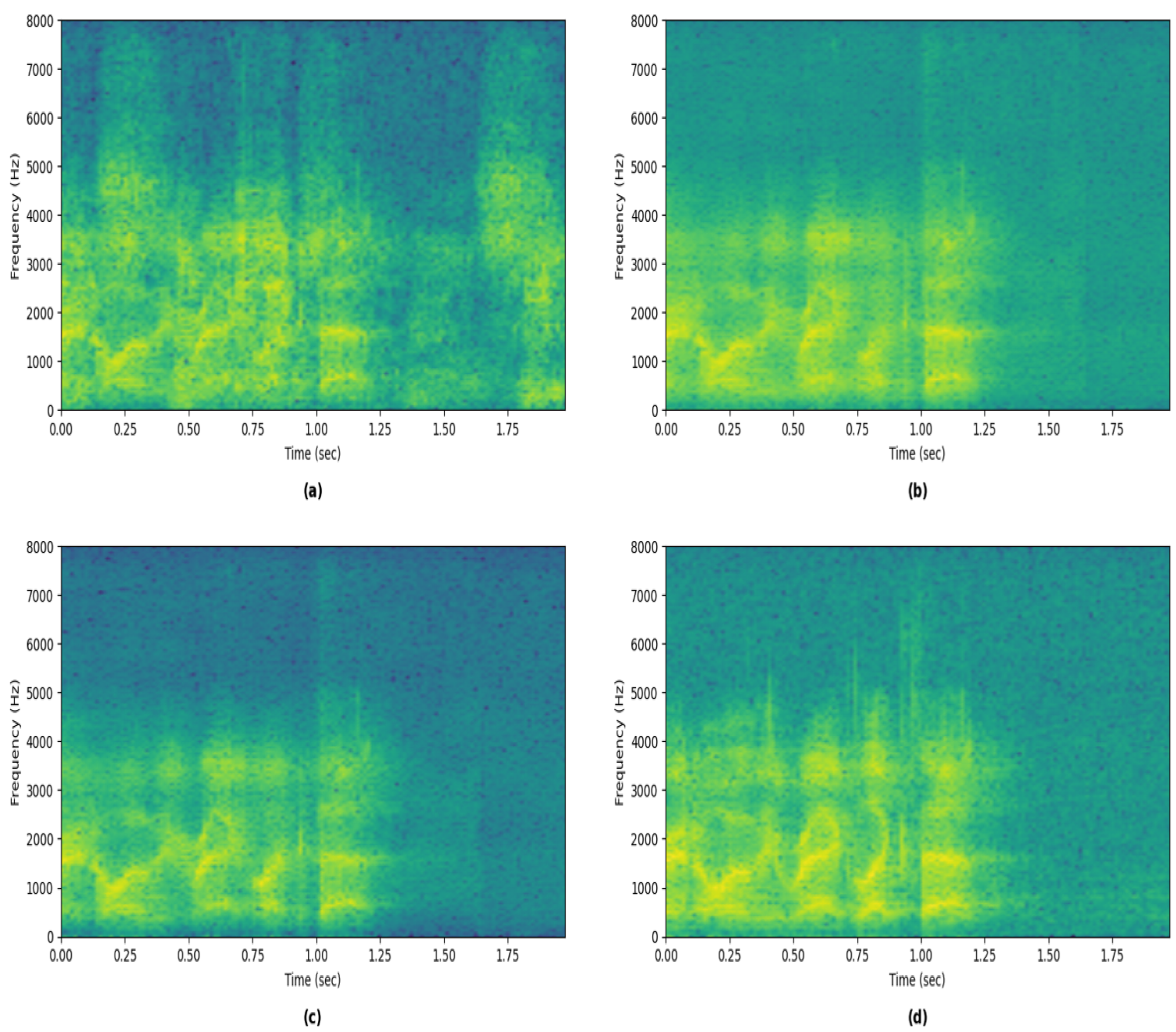
From the table, combining the DTD with the masking model improves ERLE by almost 2 dB while achieving on-par far-end only AECMOS, which indicates better echo suppression performance when there is no near-end speech. During double-talk, there is a notable increase of in the PESQ score and a minor increase of in AECMOS. These results indicate that combining the DTD with the masking model improves performance compared to not combining a DTD during double-talk periods. When adding the refinement stage to the masking+DTD stage, there is an additional improvement in all measures. Most notably, ERLE is increased by an additional dB, and PESQ is increased by . Far-end AECMOS and double-talk AECMOS are also improved, albeit by a negligible amount. It can also be observed how, without first employing the masking stage, the refinement stage on its own achieves on-par performance with the masking model without the DTD. This further asserts the efficacy of the proposed system; the masking stage, aided by the DTD, performs the initial residual echo suppression, and the refinement stage, which relies on the features provided by the masking stage, further improves performance. It can be concluded from the ablation study that the proposed configuration of the DTD aids the masking model’s performance and that the refinement stage indeed performs refinement to the outputs of the first stage since its stand-alone performance is inferior. Figure 4 shows examples of spectrograms from different stages of the system.
It can be observed from the figure that the masking model suppresses the majority of the residual echo, notably evident after s and above 4000 Hz. The finer details of the near-end speech are blurred compared to the near-end spectrogram. The refinement model refines the output of the masking model, resulting in a finer-detailed spectrogram that closely resembles the near-end spectrogram.
Next, we study different ways to combine the DTD with the masking model. We compare five different configurations:
- No double-talk detection—A single U-Net is utilized to perform spectrogram masking (similar to the proposed system, without the first U-Net).
- Configuration 1: Shared encoder—A single U-Net, where the outputs of the encoder are used both by a double-talk classifier and by the decoder that outputs the spectrogram mask. This is similar to the configuration proposed in [26].
- Configuration 2: Separate encoders, shared features—Two identical encoders are employed. The first encoder learns features used for double-talk detection. The second encoder receives all input signals, and each level’s features are concatenated with features from the matching level of the DTD’s encoder. This is similar to the configuration proposed in [17].
- Configuration 3: Separate decoders, conditioning—The features learned by a single encoder are fed into two separate decoders. The first decoder performs double-talk detection. The second decoder learns a spectrogram mask, its outputs conditioned on the DTD’s predictions by sharing the decoders’ features in each matching level. This is similar to the configuration proposed in [23].
- Proposed—the configuration proposed in this study, as detailed in Section 2.
Table 2 shows the performance of the masking model combined with the DTD in each of the above configurations. The proposed configuration achieves the best residual echo suppression performance during far-end only periods, as indicated by ERLE and AECMOS. The proposed configuration’s ERLE is more than 1 dB greater than the second-best ERLE (Conf. 3), and the AECMOS equals the no-DTD baseline AECMOS. In contrast, all other configurations see a minor degradation. In the double-talk scenario, the proposed configuration’s PESQ score is nearly greater than the second-best PESQ (Conf. 2), which is only greater than the no-DTD baseline PESQ. The AECMOS is also the highest among all compared configurations’ AECMOS. Overall, results show that the proposed configuration of DTD combined with the masking model achieves a notable performance improvement compared to not combining a DTD, where all other configurations have little to no effect on performance. We conclude that combining a DTD with the masking model is beneficial when the double-talk detection is performed before the masking and that it is necessary to learn a feature representation from the DTD’s predictions to enable the masking model to use these predictions effectively.
For completion, we provide the DTD’s performance in Table 3. Since the proposed DTD operates as a multi-label classifier where the labels are the presence of near-end speech and far-end speech, double-talk is not an actual class for the classifier. Instead, it is determined for time-frames containing both near-end and far-end speech. The provided results for near-end and far-end include time frames where both are present (double-talk). Multi-class classification results are also provided for comparison. We can observe from the table that both near-end and far-end performance is high and that precision and recall are balanced. The far-end performance is slightly better than that of the near-end. This small performance gap is expected in the low SER setting since, during double-talk periods, the near-end speech may be almost indistinguishable. This observation is also evident in the double-talk results, notably degraded. During these periods, the DTD may predict a time frame as containing far-end speech and not containing near-end speech. When using the DTD’s prediction directly as inputs to the subsequent masking model, it may cancel these time frames, as it learns to do so from the actual far-end-only time frames. Learning a representation from the DTD’s predictions helps overcome this issue. It can also be observed from the table that the proposed multi-label classifier outperforms the multi-class classifier. While near-end performance is on-par, the far-end performance and overall accuracy of the multi-label classifier are superior to that of the multi-class classifier. In the double-talk scenario, the multi-label classifier achieves superior precision and inferior recall, and its overall accuracy is notably superior to that of the multi-class classifier.
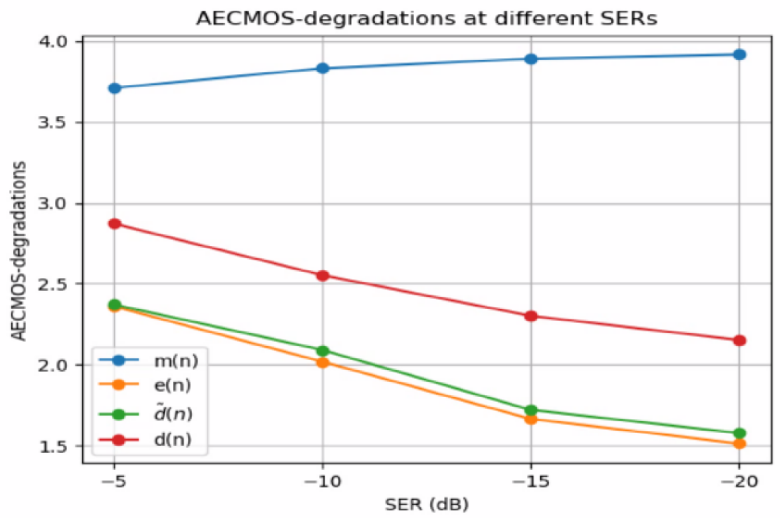
Finally, we address an issue with double-talk AECMOS-degradations in the low SER scenario. Figure 5 shows double-talk AECMOS-degradations at different SERs, where the ‘degraded’ signals used to obtain the scores are , , , and . The graphs show how the microphone signal’s AECMOS is substantially higher than the clean near-end speech’s AECMOS. Furthermore, the gap between the two is more significant when the SER is lower. When the SER is low, the far-end speech is loud (and its quality is high since we do not consider noise or additional distortions in our data), while the near-end speech is nearly indistinguishable. Thus, the microphone signal’s AECMOS-degradations are high, despite mainly containing undesired echo. On the other hand, the clean near-end speech signal’s AECMOS-degradations are considerably lower, degrading further when the SER is lowered. This may indicate that the AECMOS model was not trained on such extreme cases since we expect this score to be high regardless of the SER as it contains no noise or distortions. Nevertheless, we can see that, at all SERs, the enhanced signal obtains slightly better AECMOS-degradations than the error signal , indicating that the proposed model improves AECMOS-degradations compared to its input.
3.3. Comparative Results
We compare the proposed system to two recent RES systems: Regression-U-Net [18] and Complex-Masking [17]. Both systems operate in the T-F domain. Regression-U-Net’s inputs are the spectrogram magnitudes of and . The model predicts the spectrogram magnitudes of . Since we optimize our refinement model to increase the PESQ score, we choose in the Regression-U-Net’s implementation, as it yields the best PESQ [18]. Complex-Masking’s model consists of a convolutional encoder and decoder and a GRU between them. All layers in the model are complex, which allows the model to learn a phase-aware mask while utilizing the complete information from the input signals. The model’s inputs are the complex spectrograms of and , and its output is a complex mask applied to the spectrogram of . We note the differences between the two systems: Regression-U-Net is real-valued and performs regression (outputs the desired signal directly). At the same time, Complex-Masking is complex-valued and performs masking rather than regression. Both systems were trained using the original code provided by the authors and the same training data used to train the proposed system, and they were evaluated using the same test data. Since our work focuses on the RES part, all systems used the same preceding linear AEC. Table 4 shows the performance of the different systems, their number of parameters and memory consumption, and their real-time factor (RTF), defined as
where is the time it takes the model to infer an output for an input of duration . All systems’ RTF is measured on the standard Intel Core i7-11700K CPU GHz.
Results show that the proposed and Complex-Masking systems achieve on-par performance during far-end only periods. Complex-Masking achieves negligibly better ERLE, and the proposed system achieves negligibly better AECMOS-echo. Regression-U-Net’s performance is inferior to the other two systems - most notably, its ERLE is dB less than that of the proposed system. Regression-U-Net’s performance is also inferior to the other systems during double-talk periods. This performance gap may be due to the model’s low complexity; it has only M parameters, which is M fewer than Complex-Masking. Therefore, it may be hard for the model to learn the input-output relations in such extreme conditions properly. Contrary to far-end only periods, during double-talk, the proposed system’s performance is notably superior to that of Complex-Masking. The proposed system’s PESQ is higher by more than , and AECMOS is higher by dB. Although the proposed system’s number of parameters is about three times greater than that of Complex-Masking, its RTF is significantly lower. Thus, when inference time is a more critical constraint than memory consumption, the proposed system is favorable over Complex-Masking. It is worth noting how the proposed system’s RTF is only slightly larger than Regression-U-Net’s RTF, despite having significantly more parameters and higher memory consumption. It is due to the difference in the systems’ input sizes; the proposed model was trained on 2 s-long segments while Regression-U-Net was trained on s-long segments. Although the proposed system’s architecture allows for variable-size input, it provides the best performance for 2 s-long inputs. Thus, in cases where low memory consumption and short algorithmic delay are high priorities while performance is not, Regression-U-Net might be favorable. We also note Complex-Masking’s high RTF despite the relatively small parameter number. This is due to the complex operations, which are more time-consuming.
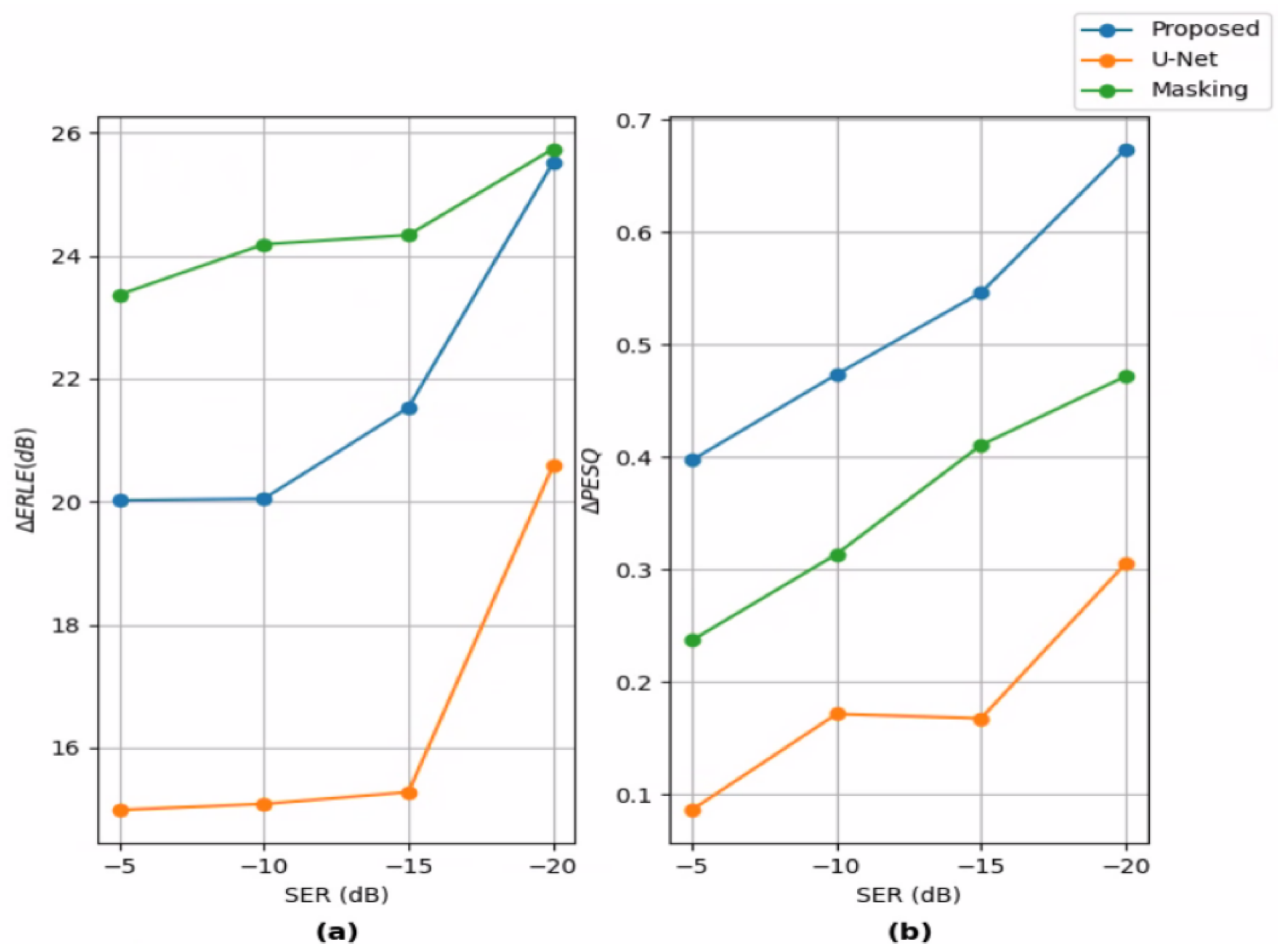
Next, we study the different systems’ performance in different SERs. We focus on far-end only ERLE and double-talk PESQ. Figure 6a shows the ERLE difference between the systems’ output signal and the error signal . Similarly, Figure 6b shows the PESQ difference.
The proposed system’s graphs show its efficiency in lower SERs - it can be seen that both and are increased when the SER is lowered, and the increase rate is also increasing (the graphs’ slopes are higher in lower SERs). In other words, the proposed system is more effective in lower SERs. A similar trend can be seen in Regression-U-Net’s performance, although the increase rate is lower. Regarding Complex-Masking, which is more comparable to the proposed system, it can be seen that although its ERLE is consistently higher than the proposed system’s ERLE, the rate at which increases is lower. At dB SER, the gap between the two graphs is negligible. The increase rate of is lower at lower SERs, while for the proposed system, it grows larger, i.e., the proposed system is more effective at lower SERs than Complex-Masking.
Finally, we compare the performance of the proposed masking architecture (AEC+M, without the DTD) with the performance of the masking architecture proposed in [28] (Masking-inpainting). Table 5 shows the different performance measures, the number of parameters, the memory consumption, and the RTF of the models.
Results show that the performance measures of the two models are on-par with negligible differences. On the contrary, the proposed model is preferable to Masking-inpainting’s model concerning memory and running-time performance. Masking-inpainting’s parameter number and memory consumption are roughly times that of AEC+M, and its RTF is an order of magnitude greater than AEC+M’s RTF. Hence the choice of the proposed masking architecture over the one proposed in [28].
4. Conclusions
We have presented a two-stage deep-learning residual echo suppression and double-talk detection system focused on the low-SER scenario. The first stage combines the DTD with a spectrogram masking model based on the U-Net architecture. We conducted experiments with different configurations (based on previous studies) of the DTD with the masking model. The results show that the proposed configuration outperforms all other configurations. To the best of our knowledge, this is the first study of different ways to combine a DTD with a residual echo suppression model and the first study to report improved results due to the DTD. The second stage performs spectrogram refinement. The architecture is based on convolution blocks consisting of residual connections. The model is optimized to maximize the desired speech quality by minimizing the PMSQE loss function, which approximates PESQ. We performed an ablation study which shows the contribution of each stage of the system. Furthermore, we conducted experiments at different levels of SER. We showed that the proposed algorithm achieves the best performance gain in the low SER setting, approving its effectiveness in this challenging scenario. Lastly, we compared the proposed system to several other systems. The proposed system outperforms all others in near-end speech quality during double-talk periods, as measured by PESQ and AECMOS. During far-end only periods, the system’s performance is on par with one of the compared systems and outperforms the other system.
Author Contributions
Conceptualization, E.S., I.C. and B.B.; methodology, E.S., I.C. and B.B.; software, E.S. and B.B.; validation, E.S.; formal analysis, E.S.; investigation, E.S., I.C. and B.B.; resources, I.C. and B.B.; data curation, E.S. and B.B.; writing—original draft preparation, E.S.; writing—review and editing, I.C. and B.B.; visualization, E.S.; supervision, I.C. and B.B.; project administration, I.C.; funding acquisition, I.C. All authors have read and agreed to the published version of the manuscript.
Funding
This research received no external funding.
Institutional Review Board Statement
Not applicable.
Informed Consent Statement
Not applicable.
Data Availability Statement
The data presented in this study are available on request from the corresponding author.
Conflicts of Interest
The authors declare no conflict of interest.
Abbreviations
The following abbreviations are used in this manuscript:
| SER | Signal-to-echo ratio |
| DTD | Double-talk detector |
| PESQ | Perceptual evaluation of speech quality |
| AEC | Acoustic echo canceller |
| DNN | Deep-learning neural network |
| BLSTM | Bi-directional long short-term memory |
| RNN | Recurrent neural-network |
| T-F | Time-freuqency |
| IRM | Ideal ratio mask |
| DTLN | Dual-signal transformation LSTM network |
| PSF | Phase-sensitive filter |
| CRN | Convolutional recurrent netowrk |
| FCRN | Fully-convolutional recurrent network |
| DFT | Discrete Fourier transform |
| VAD | Voice activity detector |
| GRU | Gated recurrent unit |
| SNR | Signal-to-noise ratio |
| PMSQE | Perceptual metric for speech quality evaluation |
| STFT | Short-time Fourier transform |
| NSLMS | Normalized sign-error least mean squares |
| NLMS | Normalized least mean squares |
| BCE | Binary cross-entropy |
| MSE | Mean squared error |
| iSTFT | Inverse STFT |
| ERLE | Echo return loss enhancement |
| AECMOS | AEC mean opinion score |
| RTF | Real-time factor |
Appendix A. Model Specifications
This appendix details the specifications of the different layers of the two DNNs discussed in Section 2. The various layers of the DTD and masking model are described in Table A1. The different layers of the refinement model are detailed in Table A2.

Table A1.
Double-talk detection and spectrogram masking model specifications. Module names with an asterisk (*) are model outputs. For down-blocks and up-blocks, the numbers in the Details column represent input channels, output channels, kernel size, and stride of the convolution window or up-sampling factor, respectively. For the GRU layer, the Details column’s numbers represent hidden-layer size and number of layers, respectively. For fully-connected (FC) layers, the number represents the number of neurons. More than one module in the Input column means concatenation of the modules in parentheses.
| Module | Details | Inst. Norm | Activation | Input |
|---|---|---|---|---|
| Down-block 1 | √ | Leaky ReLU | Model’s input | |
| Down-block 2 | √ | Leaky ReLU | Down-block 1 | |
| Down-block 3 | √ | Leaky ReLU | Down-block 2 | |
| Down-block 4 | √ | Leaky ReLU | Down-block 3 | |
| GRU | - | - | Down-block 4 | |
| FC 1 * | 2 | - | Sigmoid | GRU |
| FC 2 | 2816 | - | Leaky ReLU | GRU |
| Up-block 1 | √ | Leaky ReLU | (FC2, Down-block 3) | |
| Up-block 2 | √ | Leaky ReLU | (Up-block 1, Down-block 2) | |
| Up-block 3 | √ | Leaky ReLU | (Up-block 2, Down-block 1) | |
| Up-block 4 * | √ | Leaky ReLU | (Up-block 3, Model’s input) | |
| Down-block 5 | √ | Leaky ReLU | (Up-block 4, Model’s input) | |
| Down-block 6 | √ | Leaky ReLU | Down-block 5 | |
| Down-block 7 | √ | Leaky ReLU | Down-block 6 | |
| Down-block 8 | √ | Leaky ReLU | Down-block 7 | |
| Up-block 5 | √ | Leaky ReLU | (Down-block 8, Down-block 7) | |
| Up-block 6 | √ | Leaky ReLU | (Up-block 5, Down-block 6) | |
| Up-block 7 | √ | Leaky ReLU | (Up-block 6, Down-block 5) | |
| Up-block 8 * | - | - | (Up-block 7, Up-block 4, Model’s input) |
Table A2.
Refinement model specifications. Module names with an asterisk (*) are model outputs. For down-blocks, up-blocks and residual blocks (Res. blocks), the numbers in the Details column represent input channels, output channels, kernel size, and stride of the convolution window or up-sampling factor, respectively.
| Module | Details | Inst. Norm | Activation | Input |
|---|---|---|---|---|
| Down-block 1 | √ | ELU | Model’s input | |
| Down-block 2 | √ | ELU | Down-block 1 | |
| Res. block 1 | √ | ELU | Down-block 2 | |
| Res. block 2 | √ | ELU | Res. block 1 | |
| Res. block 3 | √ | ELU | Res. block 2 | |
| Res. block 4 | √ | ELU | Res. block 3 | |
| Res. block 5 | √ | ELU | Res. block 4 | |
| Up-block 1 | √ | ELU | Res. block 5 | |
| Up-block 2 | √ | ELU | Up-block 1 | |
| Up-block 3 * | - | - | Up-block 2 |
Appendix B. Data and Training Procedures
The independently recorded dataset was created as follows. Double-talk utterances were generated with an average overlap of and contained two different speakers. The generated dataset contains an equal amount of female and male speakers. To simulate a low SER scenario, such as a conversation over a mobile phone where the loudspeaker plays the far-end signal with high volume, Spider MT503TM or Quattro MT301TM speakerphones were employed, in which the microphone and loudspeaker are enclosed within a distance of 5 cm. In order to introduce echo path changes, in some of the recordings, the echo was played by a Logitech type Z120TM loudspeaker. The loudspeaker was moved 1, , or 2 m away from the microphone during recordings. In order to simulate near-end speech, mouth simulator type 4227-ATM of Bruel&Kjaer was employed to generate the near-end signal. Three different positions were used for the mouth simulator, either at 1, , or 2 m from the microphone. Additional variations in recording conditions include four different room sizes (between 3 × 3 × 2.5 m and 5 × 5 × 4 m) and different reverberation times (), which vary between and s. Further details concerning the recordings can be found in [18].
As mentioned in Section 2, the linear AEC operates in the subband domain. Therefore before being fed to the AEC, the input signals are transformed using uniform 32-band single-sideband filter banks [34]. The linear AEC comprises filters of 150 taps in each subband, equivalent to time-domain filters of length 150 ms with 2400 taps.
All inputs to the RES system are transformed to the time-frequency domain using a 320-point STFT with a window length of 20 ms and hop length of 10 ms. For utterances of 2 s, this results in an input tensor of size where B is the batch size, 4 corresponds to the four input signals, and 161 and 201 are the frequency and time bins, respectively. Both stages’ models are optimized with the Adam optimizer [45]. The initial learning rate of the masking model is , and the initial learning rate of the refinement model is . For both models, learning-rate scheduling is applied such that it is multiplied by a factor of each time there was no validation loss improvement for 4 consecutive epochs. Early stopping is applied if there was no validation loss improvement for 8 consecutive epochs. We set to balance the size of the two loss terms of the masking and DTD model. is set to 1 since the regularizing loss term is a magnitude-of-order smaller than . We set . For both models, the mini-batch size is 32, and the maximum number of epochs is 100. All models are implemented with Pytorch, and a single Nvidia GeForce GTX 1080 is used for training.
References
- Sondhi, M.; Morgan, D.; Hall, J. Stereophonic Acoustic Echo Cancellation-an Overview of the Fundamental Problem. IEEE Signal Process. Lett. 1995, 2, 148–151. [Google Scholar] [CrossRef]
- Benesty, J.; Gänsler, T.; Morgan, D.R.; Sondhi, M.M.; Gay, S.L. Advances in Network and Acoustic Echo Cancellation, 1st ed.; Springer: Berlin/Heidelberg, Germany, 2001. [Google Scholar]
- Zhang, H.; Wang, D. Deep Learning for Acoustic Echo Cancellation in Noisy and Double-Talk Scenarios. In Proceedings of the Interspeech 2018, Hyderabad, India, 2–6 September 2018. [Google Scholar] [CrossRef]
- Hochreiter, S.; Schmidhuber, J. Long Short-term Memory. Neural Comput. 1997, 9, 1735–1780. [Google Scholar] [CrossRef] [PubMed]
- Wang, Y.; Narayanan, A.; Wang, D. On Training Targets for Supervised Speech Separation. IEEE/ACM Trans. Audio Speech Lang. Process. 2014, 22, 1849–1858. [Google Scholar] [CrossRef] [PubMed]
- Kim, J.H.; Chang, J.H. Attention Wave-U-Net for Acoustic Echo Cancellation. In Proceedings of the Interspeech 2020, Shanghai, China, 25–29 October 2020; pp. 3969–3973. [Google Scholar]
- Ronneberger, O.; Fischer, P.; Brox, T. U-Net: Convolutional Networks for Biomedical Image Segmentation. In Proceedings of the Medical Image Computing and Computer-Assisted Intervention, Munic, Germany, 5–9 October 2015; Navab, N., Hornegger, J., Wells, W.M., Frangi, A.F., Eds.; Springer International Publishing: Cham, Switzerland, 2015; pp. 234–241. [Google Scholar] [CrossRef]
- Giri, R.; Isik, U.; Krishnaswamy, A. Attention Wave-U-Net for Speech Enhancement. In Proceedings of the IEEE Workshop on Applications of Signal Processing to Audio and Acoustics (WASPAA), New Paltz, NY, USA, 20–23 October 2019; pp. 249–253. [Google Scholar] [CrossRef]
- Westhausen, N.L.; Meyer, B.T. Acoustic Echo Cancellation with the Dual-Signal Transformation LSTM Network. In Proceedings of the IEEE International Conference on Acoustics, Speech and Signal Processing (ICASSP), Toronto, ON, Canada, 6–11 June 2021; pp. 7138–7142. [Google Scholar] [CrossRef]
- Westhausen, N.L.; Meyer, B.T. Dual-Signal Transformation LSTM Network for Real-Time Noise Suppression. arXiv 2020, arXiv:2005.07551. [Google Scholar]
- Carbajal, G.; Serizel, R.; Vincent, E.; Humbert, E. Multiple-Input Neural Network-Based Residual Echo Suppression. In Proceedings of the IEEE International Conference on Acoustics, Speech, and Signal Processing (ICASSP), Calgary, AB, Canada, 15–20 April 2018; pp. 231–235. [Google Scholar] [CrossRef]
- Erdogan, H.; Hershey, J.R.; Watanabe, S.; Le Roux, J. Phase-sensitive and Recognition-boosted Speech Separation Using Deep Recurrent Neural Networks. In Proceedings of the IEEE International Conference on Acoustics, Speech, and Signal Processing (ICASSP), Brisbane, Australia, 19–24 April 2015; pp. 708–712. [Google Scholar] [CrossRef]
- Pfeifenberger, L.; Pernkopf, F. Nonlinear Residual Echo Suppression Using a Recurrent Neural Network. In Proceedings of the Interspeech, Shanghai, China, 25–29 October 2020; pp. 3950–3954. [Google Scholar] [CrossRef]
- Chen, H.; Xiang, T.; Chen, K.; Lu, J. Nonlinear Residual Echo Suppression Based on Multi-stream Conv-TasNet. arXiv 2020, arXiv:2005.07631. [Google Scholar]
- Luo, Y.; Mesgarani, N. Conv-TasNet: Surpassing Ideal Time–Frequency Magnitude Masking for Speech Separation. IEEE/ACM Trans. Audio Speech Lang. Process. 2019, 27, 1256–1266. [Google Scholar] [CrossRef] [PubMed]
- Fazel, A.; El-Khamy, M.; Lee, J. CAD-AEC: Context-Aware Deep Acoustic Echo Cancellation. In Proceedings of the IEEE International Conference on Acoustics, Speech, and Signal Processing (ICASSP), Barcelona, Spain, 4–8 May 2020; pp. 6919–6923. [Google Scholar] [CrossRef]
- Halimeh, M.M.; Haubner, T.; Briegleb, A.; Schmidt, A.; Kellermann, W. Combining Adaptive Filtering and Complex-valued Deep Postfiltering for Acoustic Echo Cancellation. In Proceedings of the IEEE International Conference on Acoustics, Speech, and Signal Processing (ICASSP), Toronto, ON, Canada, 6–11 June 2021; pp. 121–125. [Google Scholar] [CrossRef]
- Ivry, A.; Cohen, I.; Berdugo, B. Deep Residual Echo Suppression with A Tunable Tradeoff Between Signal Distortion and Echo Suppression. In Proceedings of the IEEE International Conference on Acoustics, Speech, and Signal Processing (ICASSP), Toronto, ON, Canada, 6–11 June 2021; pp. 126–130. [Google Scholar] [CrossRef]
- Franzen, J.; Fingscheidt, T. Deep Residual Echo Suppression and Noise Reduction: A Multi-Input FCRN Approach in a Hybrid Speech Enhancement System. In Proceedings of the IEEE International Conference on Acoustics, Speech, and Signal Processing (ICASSP), Singapore, 22–27 May 2022; pp. 666–670. [Google Scholar] [CrossRef]
- Buchner, H.; Benesty, J.; Gansler, T.; Kellermann, W. Robust Extended Multidelay Filter and Double-talk Detector for Acoustic Echo Cancellation. IEEE Trans. Audio Speech Lang. Process. 2006, 14, 1633–1644. [Google Scholar] [CrossRef]
- Hamidia, M.; Amrouche, A. A New Robust Double-talk Detector Based on the Stockwell Transform for Acoustic Echo Cancellation. Digit. Signal Process. 2017, 60, 99–112. [Google Scholar] [CrossRef]
- Zhang, H.; Tan, K.; Wang, D. Deep Learning for Joint Acoustic Echo and Noise Cancellation with Nonlinear Distortions. In Proceedings of the Interspeech, Graz, Austria, 15–19 September 2019; pp. 4255–4259. [Google Scholar] [CrossRef]
- Zhou, X.; Leng, Y. Residual Acoustic Echo Suppression Based on Efficient Multi-task Convolutional Neural Network. arXiv 2020, arXiv:2009.13931. [Google Scholar]
- Ma, L.; Huang, H.; Zhao, P.; Su, T. Acoustic Echo Cancellation by Combining Adaptive Digital Filter and Recurrent Neural Network. arXiv 2020, arXiv:2005.09237. [Google Scholar]
- Chung, J.; Gulcehre, C.; Cho, K.; Bengio, Y. Empirical Evaluation of Gated Recurrent Neural Networks on Sequence Modeling. arXiv 2014, arXiv:1412.3555. [Google Scholar]
- Ma, L.; Yang, S.; Gong, Y.; Wang, X.; Wu, Z. EchoFilter: End-to-End Neural Network for Acoustic Echo Cancellation. arXiv 2021, arXiv:2105.14666. [Google Scholar]
- Zhang, S.; Wang, Z.; Sun, J.; Fu, Y.; Tian, B.; Fu, Q.; Xie, L. Multi-Task Deep Residual Echo Suppression with Echo-Aware Loss. In Proceedings of the IEEE International Conference on Acoustics, Speech, and Signal Processing (ICASSP), Singapore, 22–27 May 2022; pp. 9127–9131. [Google Scholar] [CrossRef]
- Hao, X.; Su, X.; Wen, S.; Wang, Z.; Pan, Y.; Bao, F.; Chen, W. Masking and Inpainting: A Two-Stage Speech Enhancement Approach for Low SNR and Non-Stationary Noise. In Proceedings of the IEEE International Conference on Acoustics, Speech, and Signal Processing (ICASSP), Barcelona, Spain, 4–8 May 2020; pp. 6959–6963. [Google Scholar] [CrossRef]
- Rix, A.; Beerends, J.; Hollier, M.; Hekstra, A. Perceptual Evaluation of Speech Quality (PESQ)—A New Method for Speech Quality Assessment of Telephone Networks and Codecs. In Proceedings of the IEEE International Conference on Acoustics, Speech, and Signal Processing (ICASSP), Salt Lake City, UT, USA, 7–11 May 2001; Volume 2, pp. 749–752. [Google Scholar] [CrossRef]
- Martin-Doñas, J.M.; Gomez, A.M.; Gonzalez, J.A.; Peinado, A.M. A Deep Learning Loss Function Based on the Perceptual Evaluation of the Speech Quality. IEEE Signal Process. Lett. 2018, 25, 1680–1684. [Google Scholar] [CrossRef]
- Farhang-Boroujeny, B. Adaptive Filters: Theory and Applications; John Wiley and Sons, Inc.: Hoboken, NJ, USA, 1998. [Google Scholar]
- Freire, N.; Douglas, S. Adaptive Cancellation of Geomagnetic Background Noise Using a Sign-error Normalized LMS Algorithm. In Proceedings of the IEEE International Conference on Acoustics, Speech, and Signal Processing (ICASSP), Minneapolis, MN, USA, 27–30 April 1993; Volume 3, pp. 523–526. [Google Scholar] [CrossRef]
- Pathak, N.; Panahi, I.; Devineni, P.; Briggs, R. Real Time Speech Enhancement for the Noisy MRI Environment. In Proceedings of the 2009 Annual International Conference of the IEEE Engineering in Medicine and Biology Society, Minneapolis, MN, USA, 3–6 September 2009; pp. 6950–6953. [Google Scholar] [CrossRef]
- Crochiere, R.E.; Rabiner, L.R. Section 7.6. In Multirate Digital Signal Processing; Prentice Hall PTR: Hoboken, NJ, USA, 1983. [Google Scholar]
- Koike, S. Analysis of Adaptive Filters Using Normalized Signed Regressor LMS Algorithm. IEEE Trans. Signal Process. 1999, 47, 2710–2723. [Google Scholar] [CrossRef]
- Ulyanov, D.; Vedaldi, A.; Lempitsky, V. Instance Normalization: The Missing Ingredient for Fast Stylization. arXiv 2016, arXiv:1607.08022. [Google Scholar]
- Xu, B.; Wang, N.; Chen, T.; Li, M. Empirical Evaluation of Rectified Activations in Convolutional Network. arXiv 2015, arXiv:1505.00853. [Google Scholar] [CrossRef]
- Clevert, D.A.; Unterthiner, T.; Hochreiter, S. Fast and Accurate Deep Network Learning by Exponential Linear Units (ELUs). arXiv 2016, arXiv:1511.07289. [Google Scholar] [CrossRef]
- Double-Talk Detection-Aided Residual Echo Suppression via Spectrogram Masking and Refinement GitHub Repository. Available online: https://github.com/eran-shahar/Double-talk-Detection-aided-Residual-Echo-Suppression-via-Spectrogram-Masking-and-Refinement (accessed on 8 July 2022).
- Garofolo, J.S.; Lamel, L.F.; Fisher, W.M.; Fiscus, J.G.; Pallett, D.S.; Dahlgren, N.L. DARPA TIMIT Acoustic-Phonetic Continuous Speech Corpus CDROM; NIST Speech Disc 1-1.1; Linguistic Data Consortium: Philadelphia, PA, USA, 1993. [Google Scholar]
- Panayotov, V.; Chen, G.; Povey, D.; Khudanpur, S. Librispeech: An ASR Corpus Based on Public Domain Audio Books. In Proceedings of the IEEE International Conference on Acoustics, Speech, and Signal Processing (ICASSP), Brisbane, Australia, 19–24 April 2015; pp. 5206–5210. [Google Scholar] [CrossRef]
- Sridhar, K.; Cutler, R.; Saabas, A.; Parnamaa, T.; Loide, M.; Gamper, H.; Braun, S.; Aichner, R.; Srinivasan, S. ICASSP 2021 Acoustic Echo Cancellation Challenge: Datasets, Testing Framework, and Results. In Proceedings of the IEEE International Conference on Acoustics, Speech, and Signal Processing (ICASSP), Toronto, ON, Canada, 6–11 June 2021; pp. 151–155. [Google Scholar] [CrossRef]
- Cutler, R.; Naderi, B.; Loide, M.; Sootla, S.; Saabas, A. Crowdsourcing Approach for Subjective Evaluation of Echo Impairment. In Proceedings of the IEEE International Conference on Acoustics, Speech, and Signal Processing (ICASSP), Toronto, ON, Canada, 6–11 June 2021; pp. 406–410. [Google Scholar] [CrossRef]
- Purin, M.; Sootla, S.; Sponza, M.; Saabas, A.; Cutler, R. AECMOS: A Speech Quality Assessment Metric for Echo Impairment. In Proceedings of the IEEE International Conference on Acoustics, Speech, and Signal Processing (ICASSP), Singapore, 22–27 May 2022; pp. 901–905. [Google Scholar] [CrossRef]
- Kingma, D.P.; Ba, J. Adam: A Method for Stochastic Optimization. arXiv 2017, arXiv:1412.6980. [Google Scholar] [CrossRef]
Figure 1.
Residual echo suppression setup.

Figure 2.
Structure of the double-talk detector (DTD) and masking model architecture. FC stands for fully connected.
Figure 2.
Structure of the double-talk detector (DTD) and masking model architecture. FC stands for fully connected.

Figure 3.
Structure of refinement model architecture and residual blocks. (a) Refinement model architecture. (b) Structure of the residual blocks.
Figure 3.
Structure of refinement model architecture and residual blocks. (a) Refinement model architecture. (b) Structure of the residual blocks.

Figure 4.
Visualization of spectrograms of the different stages’ outputs. (a) Error signal spectrogram. (b) Spectrogram of the signal reconstructed from the masking stage’s output. (c) Spectrogram of the refinement stage’s output. (d) Near-end signal’s spectrogram.
Figure 4.
Visualization of spectrograms of the different stages’ outputs. (a) Error signal spectrogram. (b) Spectrogram of the signal reconstructed from the masking stage’s output. (c) Spectrogram of the refinement stage’s output. (d) Near-end signal’s spectrogram.

Figure 5.
AECMOS-degradations of the different signals at various signal-to-echo ratios (SERs).

Figure 6.
Systems’ performance in different SERs. (a) Echo return loss enhancement (ERLE) difference between the systems’ outputs and the error signal. (b) Perceptual evaluation of speech quality (PESQ) difference between the systems’ outputs and the error signal.
Figure 6.
Systems’ performance in different SERs. (a) Echo return loss enhancement (ERLE) difference between the systems’ outputs and the error signal. (b) Perceptual evaluation of speech quality (PESQ) difference between the systems’ outputs and the error signal.

Table 1.
Ablation study results. M stands for masking, D for DTD, and R for refinement.
| Far-End Only | Double-Talk | |||
|---|---|---|---|---|
| ERLE | AECMOS | PESQ | AECMOS | |
| AEC | ||||
| AEC+M | ||||
| AEC+M+D | ||||
| AEC+R | ||||
| AEC+M+D+R | ||||
Table 2.
Study of different configurations of the masking model with a DTD. Conf. stands for configuration.
Table 2.
Study of different configurations of the masking model with a DTD. Conf. stands for configuration.
| Far-End Only | Double-Talk | |||
|---|---|---|---|---|
| ERLE | AECMOS | PESQ | AECMOS | |
| No DTD | ||||
| Conf. 1 | ||||
| Conf. 2 | ||||
| Conf. 3 | ||||
| Proposed | ||||
Table 3.
Performance of the DTD. Numbers in parentheses represent the respective results of the multi-class classifier.
Table 3.
Performance of the DTD. Numbers in parentheses represent the respective results of the multi-class classifier.
| Precision | Recall | Accuracy | |
|---|---|---|---|
| Near-end | |||
| Far-end | |||
| Double-talk | |||
| Overall | - | - |
Table 4.
Comparison of the proposed, the Residual-U-Net (U-Net), and the Complex-Masking (Masking) systems. Param. stands for parameters and Mem. for memory.
Table 4.
Comparison of the proposed, the Residual-U-Net (U-Net), and the Complex-Masking (Masking) systems. Param. stands for parameters and Mem. for memory.
| Far-End Only | Double-Talk | # Param. | Mem. | RTF | |||
|---|---|---|---|---|---|---|---|
| ERLE | AECMOS | PESQ | AECMOS | (Bytes) | |||
| U-Net | M | M | |||||
| Masking | M | M | |||||
| Proposed | M | M | |||||
Table 5.
Comparison of the proposed masking architecture without the DTD (AEC+M) and the masking architecture in Masking-inpainting.
Table 5.
Comparison of the proposed masking architecture without the DTD (AEC+M) and the masking architecture in Masking-inpainting.
| Far-End Only | Double-Talk | # | Mem. | RTF | |||
|---|---|---|---|---|---|---|---|
| ERLE | AECMOS | PESQ | AECMOS | Param. | (Bytes) | ||
| Masking-inpainting | M | M | |||||
| AEC+M | M | M | |||||
Publisher’s Note: MDPI stays neutral with regard to jurisdictional claims in published maps and institutional affiliations. |
© 2022 by the authors. Licensee MDPI, Basel, Switzerland. This article is an open access article distributed under the terms and conditions of the Creative Commons Attribution (CC BY) license (https://creativecommons.org/licenses/by/4.0/).
Share and Cite
MDPI and ACS Style
Shachar, E.; Cohen, I.; Berdugo, B. Double-Talk Detection-Aided Residual Echo Suppression via Spectrogram Masking and Refinement. Acoustics 2022, 4, 637-655. https://doi.org/10.3390/acoustics4030039
AMA Style
Shachar E, Cohen I, Berdugo B. Double-Talk Detection-Aided Residual Echo Suppression via Spectrogram Masking and Refinement. Acoustics. 2022; 4(3):637-655. https://doi.org/10.3390/acoustics4030039
Chicago/Turabian StyleShachar, Eran, Israel Cohen, and Baruch Berdugo. 2022. "Double-Talk Detection-Aided Residual Echo Suppression via Spectrogram Masking and Refinement" Acoustics 4, no. 3: 637-655. https://doi.org/10.3390/acoustics4030039