Wave Mode Identification of Acoustic Emission Signals Using Phase Analysis


1
Structural Integrity & Composites Group, Faculty of Aerospace Engineering, Delft University of Technology, Kluyverweg 1, 2629 HS Delft, The Netherlands
2
School of Aerospace, Transport and Manufacturing, Cranfield University, Bedfordshire MK430AL, UK
3
Aerospace Research Centre, National Research Council Canada, Ottawa, ON K1A0R6, Canada
4
Department of Mechanical and Aeronautical Engineering, Clarkson University, Potsdam, NY 13699, USA
*
Author to whom correspondence should be addressed.
Acoustics 2019, 1(2), 450-472; https://doi.org/10.3390/acoustics1020026
Submission received: 9 May 2019
/
Revised: 8 June 2019
/
Accepted: 12 June 2019
/
Published: 15 June 2019
Abstract
:Acoustic Emission (AE) monitoring can be used to detect and locate structural damage such as growing fatigue cracks. The accuracy of damage location and consequently the inference of its significance for damage assessment is dependent on the wave propagation properties in terms of wave velocity, dispersion, attenuation and wave mode conversion. These behaviors are understood and accounted for in simplistic structures; however, actual structures are geometrically complex, with components comprising of different materials. One of the key challenges in such scenarios is the ability to positively identify wave modes and correctly associate their properties for damage location analysis. In this study, a novel method for wave mode identification is presented based on phase and instantaneous frequency analysis. Finite Element (FE) simulations and experiments on a representative aircraft wing structure were conducted to evaluate the performance of the technique. The results show how a phase analysis obtained from a Hilbert Transform of the wave signal in combination with variations of the instantaneous frequency of the wave signal, can be used to determine the arrival and therefore identification of the different wave modes on a complex structure. The methodology outlined in this paper was proven on an Automatic Sensor Test wave signal, Pencil Lead Breaks and Hanning windows and it was shown that the percentage difference is between 3% and 15% for the A0 and S0 wave speed respectively.
1. Introduction
The Acoustic Emission (AE) technique is recognized as a potential passive Structural Health Monitoring (SHM) tool. It is capable of detecting and locating damage by sensing stress waves that are dynamically generated from different mechanisms in the damage formation process. The prevalence of AE waves from these sources is a function of the material properties, structural geometry and loading configuration [1,2]. Gagar et al. conducted a study on the effects of mechanical loading and geometrical complexity on AE generation during fatigue crack growth [1]. It was observed that there were significant variations in the rates of AE signal generation during crack progression from initiation to final failure, with a number of distinct phases identified and associated with different failure mechanisms operating at particular stages in the failure process. In metals, the mechanisms responsible for AE generation during fatigue crack growth include: crack extension [3,4], deformation of plastic zone [5] and fretting of fractured surfaces [6,7].
In composite materials, AE signals can be potentially generated due to matrix cracking, delamination, fiber breakage and macroscopic fracture [8]. Material properties and component geometry can affect the dispersion properties of AE, where the propagating velocity of the extensional and flexural wave modes changes with frequency in thin structures such as aircraft skins [9]. Typically, this relation can be determined analytically for simple plate-like structures; however, these equations rapidly become very complicated with increased geometrical complexity of the structure [10,11,12,13,14,15].
Damage location can be performed using arrival time of these stress waves at known sensor locations. The performance of the AE technique for damage detection and location can potentially be influenced by different factors in each of the stages of the monitoring process, the AE signal source, propagation medium, signal detection and data processing. Parameters required for accurate damage location include the sensor location coordinates and the propagating wave speed. A primary challenge in locating damage is the ability to identify the detected wave modes and correctly associate their properties in terms of their speed. This is a fundamental requirement for the AE source location algorithms such as the Geiger method [16].
This challenge is further compounded with complex geometry and increased wave propagation distance where the effects of reflection, attenuation [17] and dispersion [18] can be pronounced. Furthermore, additional effects include dispersion due to material anisotropy [19], as well as wave mode conversion, where a particular wave mode changes to another; and complexities in the geometry of the structure [11,20].
Several methods are found in the literature assessing the modes identification. Some of the most common methods are based on the time-frequency representation, or spectrogram of the waves received at different sensing locations. This information provides a time evolution of the energy of different frequency components at each sensor location. At waves arrival, the energy reaches maximum values for the frequency band of the signal. If the spectrogram is obtained from signals with known source locations, then with the distances known time can be converted to velocity, and they provide an experimental calculation of the dispersion curves. The spectrogram can be calculated by Matching Pursuit (MP), Sort Time Fourier Transform (STFT) [21], Wavelet Transform (WT) [22], Wigner-Ville Distribution Transform (WVDT) [23]. The frequency-wavenumber representation also provides the separation of the wave modes, and can be calculated for example with a two-dimensional FFT (2D-FFT), although this method needs the availability of a greater number of sensors [24].
Baxter et al. [25] developed an experimental method for wave velocity calibration using repeated Pencil Lead Breaks (PLBs) at various locations, where the time difference of arrival of AE signals received at an array of sensors is mapped across the monitored area of the structure, creating a reference table with which to perform damage location. This method demonstrated improved damage location accuracy in anisotropic test samples containing complex geometric features, as compared to the nominal approach of assuming a uniform wave velocity. The main drawback is that the calibration source used is not entirely representative of AE signals dynamically generated from actual damage events, resulting in significantly different propagation response. Haider et al. [26] developed an analytical method to predict AE waveforms from many different AE sources, based on Helmholtz excitation potentials. Their research included an extensive analysis of some influencing parameters, and specific results for AE from crack propagation and bulk AE, concluding that experimental bulk AE may be neglected, and that further investigation is needed towards a better prediction of the amplitude of the different modes.
Furthermore, the broadband and multi-modal nature of the AE signal presents a significant challenge in positively verifying the wave mode captured using a fixed threshold detection method.
The selection of the fixed threshold value in a complex structure requires the AE operator to perform a series of noise test levels in order to understand the background noise in the system under consideration. It is common to add 5 to 6 dB as suggested in [27]. This allows the operator to set a threshold value, however, it is important to understand that this selection is somewhat arbitrary.
The capability of the AE technique has been demonstrated successfully in simple test components [1]. However, realistic structures like aircraft wings, which consist of assemblies of different components, complex geometries, as well as different materials, provide a more challenging environment for the AE technique. The National Research Council Canada (NRC) has developed several test platforms capable of closely replicating realistic structures in terms of materials, geometries and fatigue loading conditions [28], such as the aircraft wing box analyzed in the present study. Multiple PLB tests were performed on this structure in order to understand which wave speed (S0 vs. A0) was being triggered for a specific threshold value. Unfortunately, when the threshold is crossed by the S0 or A0 wave packet, it is unclear which one actually triggered the recording of the emission. Additionally, a different calibration test (i.e., Hanning Window or Pencil Lead Break), such as an Automatic Sensor Test (AST), also threshold based, is known to produce different results as the amplitude of the S0 and/or A0 wave signal is frequency dependent [29].
These unknowns led the authors to develop a reliable methodology that could be used repeatedly in a complex structure to identify the correct wave mode, for wave velocity calibration and damage/source location. In this paper this novel method is presented for Lamb wave modes identification by finding the arrival of different wave packets indicated by abrupt phase variations and instantaneous frequency discontinuities. One of its advantages is the simplicity of its application, consisting in the extraction of the phase information from the Hilbert Transform (HT) of the signal, and its derivative with time, the instantaneous frequency finst, as it will be explained in Section 3 of this manuscript. An algorithm is then designed to detect abrupt phase variations, which need to be verified by the corresponding finst discontinuities. The main advantage of this method is its sensitivity to small phase changes—in case of two interfering waves with the same frequency content, which means having the same temporal variation of phase with time, the arrival of the second wave can be detected by a change in phase. One of the challenges faced by AE operators is that AST Signals, PLB and Hanning Windows generate waves in which the amplitude of the S0 and A0 are frequency dependent [29]. The methodology outlined in this study provides a means of selecting the correct wave mode (S0 and/or A0) and thus guide the user on the proper selection of a threshold value for a specific mode (wave speed), which would lead to a more accurate emission location [1]. The Pencil Lead Break (PLB) and Automatic Sensor Test (AST) signals propagating in the realistic wing-box structure aforementioned are used for validation of the proposed methodology.
2. Experimental Setup
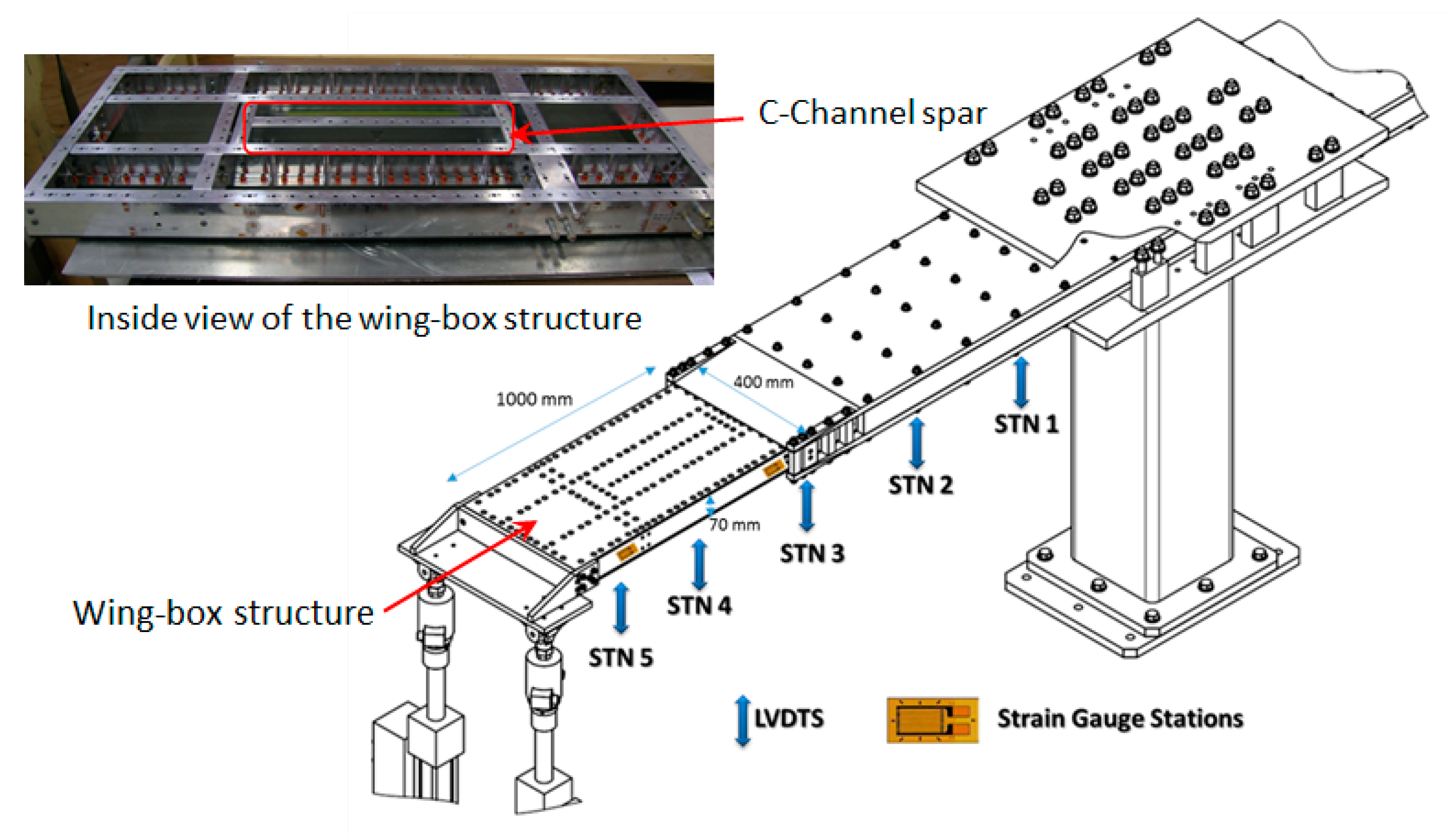
The experimental setup in this study made use of NRC’s SHM test platform, as shown in Figure 1. The platform consists of a wing-box structure with dimensions of approximately 1000 mm by 400 mm by 70 mm comprising of fastened ribs and spars manufactured from aluminum AA6061-T6 and Carbon Fiber Reinforced Polymer (CFRP) skin. The replaceable C-Channel spar, as shown in Figure 1 was manufactured from aluminum AA7075. The upper and lower CFRP skin panels consisted of 36 plies (approx. 0.1321 mm per ply for a total thickness of 4.75 mm) with a layup sequence of [45/45/-45/-45/90/90/0/0/45/-45/0/0/45/-45/45/-45/0/0]s and ply properties as specified in Table 1 [30,31]. The lower wing skin structure is fastened to the spars/ribs using Hi-LokTM fasteners, while the upper skin is secured using removable fasteners and nut plates, allowing both access to the inner structure of the wing box, as well as the opportunity for the replacement of the damaged C-Channel test spar, as shown in Figure 1, once the test was completed.
A multi-channel Physical Acoustics AE system was used with broadband piezoelectric sensors to record AE data generated throughout the tests with a sampling rate of 5 MS/s. Pre-amplifier gain for each channel was set at 40 dB and the AE signal detection threshold was set at 45 dB. The WD-100–900 kHz wideband PZT transducers from Physical Acoustics Inc. were used in this study. These transducers have an operating frequency range from 125–1000 kHz, a resonant frequency of 125 kHz and a peak sensitivity of 56 dB as shown in [32]. The transducers have an overall general dimension of 18 mm outer diameter by 17 mm in height. The case material of the transducers is stainless steel. They are connected to the AE system via a Bayonet Neill–Concelman (BNC) connector. The AE system consisted of an 8 channel PCI-2 board and system also manufactured by Physical Acoustics Inc. [33]. A two-sensor AE event location setup (1D) was used to monitor the test sample with the sensors attached to the web of the test spar using Dow Corning RTV 3140 silicone rubber. This pair of sensors on the test sample is also referred to as Location Group 1, consisting of Sensors 1 and 2. Another pair of sensors was installed on the adjacent spar, consisting of Sensors 3 and 4, which are referred to as Location Group 2. A schematic of the wing-box layout, and the AE sensor arrays are illustrated in Figure 2. The C-Channel has 15 fastener holes along its length.
As shown in Figure 2, Sensors 1 and 2 were placed as far away from each other as possible in order to maximize the sensor coverage area, which spanned from Holes 3 to 13. The sensors on the adjacent spar, Sensors 3 and 4 were located in the same longitudinal positions. The locations of the sensors and fastener holes along the test spar and the wing-box structure are provided in Table 2.
3. Wave Mode Identification Methodology
Guided Lamb waves are multimodal, i.e., the number of modes being excited depends on the excitation frequency. For most practical purposes, only the first symmetric (S0) and anti-symmetric (A0) wave modes are used. These fundamental wave modes are independent of each other and propagate at different velocities. Due to different propagation velocities of the A0 and S0 waves, the time between the arrivals of the A0 and S0 wave modes gets larger with increasing propagation distance. A sufficient distance between the source and the sensor may completely separate these waveforms, in which case the starting and ending instants of each mode can be detected. In this situation, where the wave modes are separated, several methods are found in the literature for finding the Time of Arrival (ToA), such as: the Akaike Information Criterion (AIC) [34,35], the threshold and rising edge of the envelope slope [36]. Bai et al. offered a comparative analysis between the aforementioned techniques and time correlation, Continuous-time Wavelet Transform (CWT) correlation and CWT binary map for wave mode identification [37].
However, in case of waveforms overlapping due to reflections from the boundaries or between modes, the time domain signal analysis will not be sufficient for the ToA determination. The method presented in this work for mode separation is based on the phase analysis from the Hilbert Transform (HT) calculated using Fast Fourier Transform (FFT), and inverse FFT, as the basis for wave mode identification in complex structures, as shown in Figure 3.
3.1. Hilbert Transform Calculation for Phase and Instantaneous Frequency Analysis
The Hilbert Transform (HT) is used for the calculation of the analytic signal xa(t) of a given real signal xr(t). The result is a complex signal whose real part coincides with the original signal [38], while the imaginary part is its HT, provided in Equation (1) as:
where j is the imaginary unit, and H[xr(t)] is the HT of xr(t).
The imaginary part in Equation (1) is such that the frequency spectrum of the analytic signal has zero amplitude in the negative frequency range. In the positive frequency range, the spectrum of the analytic signal coincides with the spectrum of the real signal, with twice the energy to compensate for the loss of spectral energy from the negative frequencies. In order to accomplish this definition, the imaginary part xHT(t) is a ±90° shifted version of the real signal. The shift is positive for negative frequencies and vice-versa. In the frequency domain, with angular frequency ω, this shift is equivalent to multiplying by ±j, imaginary unit, and therefore, the imaginary part of the analytic signal can be obtained from the original signal in the frequency domain Xr(ω) as described by Equation (2).
where Xr(ω) is the FFT of xr(t). With the definition of the HT in the frequency domain provided in Equation (2), the analytic signal results in Equation (3).
The analytic signal xa(t) so described may be generated based on the Fast Fourier Transform (FFT). This method has also the advantage of generating xa(t) and xHT(t) at the same time. As followed in Equation (4), after the FFT of xr(t) is performed, the amplitudes of the negative frequency components are set to 0, and the amplitudes of the positive frequencies are multiplied by 2, obtaining Xa(ω). Finally, the inverse FFT is applied to the resulting function in order to get the analytic signal back in the time domain.
The magnitude of this signal xa(t) is the envelope of the original real signal, while the argument corresponds to its phase, as provided in Equation (5).
The phase of a signal or wave packet with a dominant or central frequency fc, increases linearly with time, at a rate that is proportional to this frequency. In other words, the variation of the phase of a signal with respect to time approximates its instantaneous circular frequency ωinst(t), calculated from the phase of its analytic signal as:
where finst is the instantaneous frequency.
As an example of the application of these calculations, Figure 4 shows a numerical example of the arrival of mode S0 (tS0), its reflections from the boundaries (tRS0), and mode A0 (tA0), at three different arbitrary frequencies f1–f3.
In Figure 4a, the three waves overlap at a specific instant, depending on their frequencies and the travelling distance. This overlapping makes it challenging to determine the instant of time when the second or third waveform starts due to constructive and destructive effects of wave overlapping. In this situation, the methods based on signal analyzed in time domain or envelope slope are not enough for the determination of the arrival time of each of these waves.
The phase analysis of the signal obtained from the Hilbert Transform (HT) is proposed for modes separation and later identification in this paper. The start of a wave packet interfering with noise and/or a different wave packet is characterized by a variation on the evolution of the phase of the signal, and the corresponding frequency change, as shown in Figure 4b,c respectively. These changes are also present at the end of the wave packet, which is an indication of its duration. In the case of Lamb waves, both S0 and A0 modes can be identified by their respective phase changes.
It is not possible to experimentally excite a signal at a single frequency. Hence a bandwidth around the central or dominant frequency will always be present. The first consequence is that the instantaneous frequency of a wave packet cannot be a single value, contrary to what is shown in Figure 4c. As such, a small variation around the dominant frequency is expected.
When two waveforms of different central frequency are overlapped, the resulting instantaneous frequency is a value between the frequencies of the overlapping waves. Hence, the instant when a waveform of central frequency fC2 is overlapped with a waveform of central frequency fC1 can be detected by an instant change in the slope of the phase, and the corresponding change in the finst(t), as depicted in Figure 5.
Figure 5a shows an example of the amplitude, phase and instantaneous frequency of an experimentally obtained waveform. The waveform has two different central frequencies at 50 kHz and 150 kHz respectively, as indicated by the FFT of the signal in Figure 5c. Referring to Figure 5a, instant (1) is the arrival of the first wave packet at central frequency 50 kHz, indicated by the sudden change in the phase slope, where the constant derivative of the slope suddenly changes. This instant is highlighted within an ellipse in Figure 5b, the magnified view of instant (1). This sudden variation on the phase of the signal generates a significant variation of its derivative with time, or instantaneous frequency as it is defined by Equation (6). This derivative may take positive or negative values. Instant (1) is an example of a negative derivative, followed by the constant phase variation at frequency 50 kHz. Instant (2) corresponds to the arrival of a wave at frequency 150 kHz, interfering with the end of the wave at 50 kHz. Instant (3) is the arrival of a second wave at 150 kHz, interfering with the previous one. Instants (4) and (5) are examples of the interference of wave packets at 50 and 150 kHz, indicated by the different slopes of the phase plot. Higher slopes correspond to higher frequencies, or faster variation of phase with time.
In the case of a broadband signal, there are multiple frequencies contributing to a varying instantaneous frequency. This variation in the instantaneous frequency is no longer constant, as it would for a central frequency signal, and yet it results in a clear phase slope variation at the arrival of the very first wave packet, the S0 mode. However, the overlapping of the different frequency components, together with the interference of the multiple reflections from the complex geometry of the structure, complicates the separation of the individual wave packets, and therefore the clear identification of mode A0. As such, phase analysis by Hilbert Transform (HT) is then combined with dispersion curves and geometry considerations, for wave mode identification.
The process followed for the mode identification using phase analysis, either for central frequency content or broadband signals, in simple or complex structures is summarized in Figure 6. The HT of the AE provides the phase of the signal, and its instantaneous frequency calculated as the variation of phase with time. The arrival of the first wave packet is identified by the first sudden change in the slope of the phase, and the corresponding instantaneous frequency peak. In the propagation of Lamb waves, mode S0 is the fastest mode and therefore this first change in phase indicates the ToA of mode S0. Knowing the distance between the AE source and the sensor provides the wave velocity of mode S0.
For simple geometries, like flat plates, the distances between AE and sensor are easy to determine. If the geometry is complex, the most direct propagation path needs to consider the different structural parts. The velocity of mode S0 calculated in this manner is an average velocity for this propagation path.
The consecutive changes in phase are due to mode A0 and the reflections of both S0 and A0 with the geometric boundaries. The ToA of the reflections of mode S0 are estimated from the velocity of propagation of this mode already obtained and geometry considerations, that is the distances of the reflecting elements (edges, stiffeners, etc.) to the sensor. Then the corresponding S0 and RS0 changes of phase (and instantaneous frequency) are discriminated and excluded for the identification of ToA of mode A0.
This procedure for modes identification can be quite straightforward for narrow band frequency signals, and simple geometries, in which case distances to boundaries and directions of propagation have a relatively simple determination. However, it gets complicated when applied to complex geometries and broadband signals. The ToA of the AE reaching a particular sensor is accurately determined by the sudden change in phase upon arrival, as described in Section 3.1. This is the time for mode S0 to propagate following the direct propagation path between source and sensor. This velocity that is accurately determined, is then assumed as an average of the velocity for this path and its surrounding area, where the possible closest reflections can be generated and arrive at the sensor before the arrival of mode A0. This velocity is then used in the calculation of the ToA of the closest possible reflections susceptible to interfere with A0. Once these ToA are calculated, their corresponding phase and instantaneous frequency events are discarded for the consideration of ToA of A0. An approximation of the Dispersion Curves (DCs) and a pre-analysis of the frequency content of the AE, such as the frequency spectrum from the FFT of the signal, provide a first approximation of the velocity of mode A0, named vA0*, and from this an approximation of its ToA, tA0*. Then the nearest phase change instant, after discarding the S0 reflections, is picked as a correction of this approximate ToA. In the present analysis the AST test results served as such additional means of validation.
In some occasions the phase changes are not easily detected at a first glance. That is the main reason for the combination of phase and instantaneous frequency within the same analysis. There are small fluctuations in phase, some of them due to noise, some due to the frequency dependency of the Hilbert Transform. A still small variation in phase, but in this case due to the interference of 2 waves, can be more prominent and easier to detect from its 1st derivative, which is the instantaneous frequency. Once the instantaneous frequency marks this instant as an event of interest, a closer observation of the phase evolution shows a change more pronounced than expected as the phase variation for a single wave packet.
3.2. Wave Calibration between Automatic Sensor Test (AST), Pencil Lead Break (PLB) and Phase Analysis
The assumption of using the standard wave speeds commonly found in the literature for specific material would result in incorrect location of the emissions captured by the Acoustic Emission (AE) system, especially in complex multi-material structures. As part of implementing AE on any structure, it is standard to perform Pencil Lead Break (PLB) and Automatic Sensor Test (AST) prior to acquiring data from that structure. An AE operator will perform a calibration by identifying the location of the AST and/or PLB with respect to the sensor placement. This study makes use of these two types of signals while following the method described in the previous section in order to identify the corresponding wave modes. AST, PLB, or cracks emanating in a thin plate-like structure contain several Lamb waves modes excited at wide range of frequencies. For most practical purposes, the frequency range is below the first cut-off frequency, where only the fundamental symmetric (S0) and anti-symmetric (A0) Lamb modes are considered.
The AST within the Physical Acoustic system [39] consists of an acoustic pulse sent from a known actuation location, receiving the response to this actuation at another known location, which allows for the determination of the propagating average speed in the structure along its path. Two different paths (Sensors 1–4) were evaluated in both directions of propagation, obtaining the Time of Arrival (ToA) by setting the detection amplitude threshold at 45 dB. The average ToA was obtained from the responses to 50 AST pulses.
PLB on the other hand, consists of the reception of eight PLB events at two pairs of sensors, named Location Group 1 and Location Group 2 shown in Figure 2. Four of the PLB events were performed at Hole 3 location, and the other four events at Hole 4. The ToA were obtained with an amplitude threshold of 45 dB and an average of four events at each PLB location.
The experimental results from the PLB were additionally analyzed in phase domain through the HT operator. The ToA of mode S0 was accurately calculated, while mode A0 was interfering with the multiple reflections corresponding to the complex geometry, and the high dispersion due to the broadband frequency. Therefore, the amplitude threshold results from AST and PLB were used as a first approximation for the identification of the phase variations due to the A0 wave arrival.
Despite the broadband range of frequencies, the Fast Fourier Transform (FFT) of the PLB signals revealed the existence of a predominant frequency. This frequency was then used as central frequency of the excitation signal in the Finite Element Model (FEM) developed for the analysis of the waves propagation in this complex structure.
4. Finite Element Model
A representative model of the wing-box mid-section was created to perform a Lamb wave propagation study using ABAQUS CAE™. The primary objective of this model was to obtain an approximate representation of the complex wave propagation in this 3D structure. ABAQUS implicit method was employed in this study. The model consisted of three adjacent spars made from AA7075, top and bottom Carbon Fiber Reinforced Polymer (CFRP) skins (4.75 mm thick), in addition to five piezoelectric transducers: four working as sensors and one as actuator, as shown in Figure 7. The overall size of the model was approximately 495 mm × 208 mm × 62 mm (mid-section of the entire wing box). Attenuation properties of the CFRP skins were not considered in this model to minimize complexity.
The piezoelectric transducers were 6.5 mm thick, with diameter of 20 mm and a density of 7850 kg/m3. The piezoelectric actuator/sensors were assigned orthotropic piezoelectric material properties. These and other properties are gathered in Table 3.
Pairs of piezoelectric sensors were positioned on the web of each spar, locations of which are provided in Table 2. A tie constraint was set in the model between the CFRP skins and the aluminum spars. A fixed constraint was also set around the outer edges of the wing-box substructure to simulate the rigid nature of the structure, as shown in Figure 7. An FFT of a PLB signal showed the existence of a dominant frequency of the PLB tests for this structure, close to 110 kHz. As such, a central frequency of 110 kHz was selected for the FEM study. A piezoelectric actuator was positioned on the upper flange of the middle spar to simulate the AE signal. The excitation signal consisted of a 5 cycle Hanning window tone burst at 110 kHz.
The entire geometry was meshed using element size less than 1 mm, and the simulation was set to run with a time step of 0.1 μs. The selection of the element size and time step represents a compromise between computing time and that proposed in [10,42], where a minimum of 20 points per cycle of the highest frequency and a minimum of 10 nodes per wavelength are recommended for sufficient temporal and spatial resolution. The FEM consisted of a total of 144,044 hexahedral linear elements (C3D8R), 1200 linear hexahedral elements of type C3D8E (piezoelectric), and 56,856 linear quadrilateral elements of type S4R (shell elements for the skins) for a total of 202,100 elements.
A Windows 7 computer server with two Intel Xeon CPU 2650V3 (a total of 20 physical CPUs) running at 2.30 GHz with 128 Gigabytes of RAM was used in this study, where the simulations took over seven days to run for a total simulation time window of 400 microseconds.
5. Results
5.1. Wave Velocity Calibration
Three methods were used for the ToA determination of the acoustic waves propagating in the complex wing-box structure. The first two methods are based on the Automatic Sensor Test (AST) and the Pencil Lead Break (PLB) tests, both of which are experimental, based on the amplitude of the waves received by several sensors. The arrival of the wave is detected by setting an amplitude threshold in the time domain. In the third method, the PLB results are analyzed in the phase domain, using the methodology presented in this paper.
5.1.1. Dispersion Curves and Frequency Range
As mentioned in the flowchart in Figure 6, the dispersion curves are used as a means of validation of the wave modes identification, detected by the AST and PLB tests. The dispersion curves for the materials present in the wing-box structure together with the range of frequencies expected in the aforementioned tests, give an approximated range of corresponding velocities of modes S0 and A0.
The range of frequencies is obtained from the frequency content of the PLB signals. Given that the AST waveforms were not recorded, this could not be assessed. The eight events from the two PLB locations revealed similar FFT results. As an example, Figure 8 shows the Fast Fourier Transform (FFT) for one of the four PLB events, event #1 in this case (ev1), at hole 3 (H3), detected by Sensors S1–S4, whose dominant frequencies were found to be around 110 kHz, the frequency that was chosen for the FEM analysis.
The FFT of the event as depicted in Figure 8b shows a low frequency modulation around 30 kHz, occurring mainly in sensor 4, and with much lower intensity in the other three sensors, as shown by the four sensors synchronization of the low frequency content in Figure 8a; an indication that this frequency may have been external to the test itself, and therefore not considered for the analysis. The overall frequency range of the PLB tests considered for the DCs was approximately 30–350 kHz (See Figure 8b).
The dispersion curves were calculated under the assumption of isotropic aluminum AA7075T6 and CFRP. Table 4 gives the velocity ranges of each of the materials, considering the parts’ thicknesses, for the frequency range of interest.
5.1.2. ToA from Automatic Sensor Test (AST)
In the case of the AST signals, the pre-amplification gain was set to 40 dB, and detection threshold was set to and 45 dB, that is 5 dB over the background noise magnitude received by each channel [27]. Table 5 shows the AST results for ToA determination from this experiment.
The average wave velocity estimated with the AST method is approximately vAST = 2691 m/s, which according to the DCs results in Table 4 corresponds to the A0 wave mode. It is important to note that, at the time of the experimental campaign, the entire waveforms of the AST signals were not recorded and only the time interval between sensors and received signal amplitude were captured in a database [43]. Therefore, due to the lack of the entire waveform for the AST signal, phase analysis could not be conducted.
5.1.3. ToA from Pencil Lead Break (PLB)
In this case, the wave from a PLB at a known location was received at two different sensors. The time delay between the two sensors, and their distance relative to the PLB location dPLB, were used for determining the wave velocity. The ToA calculation uses the time data from the first peak above the 45 dB threshold. Four PLB tests were performed at fastener Holes 3 and 4. The average wave velocities were found to be approximately 5359 and 5280 m/s for the PLB at holes 3 and 4 respectively, as provided in Table 6. The overall average from the amplitude threshold results in a wave velocity of approximately vPLB = 5319 m/s, corresponding to the S0 wave mode in accordance with DCs in Table 4.
Figure 9 shows an example of the PLB signals generated at hole 4 and gathered by Sensors 1 and 2. The zoomed in view shows the 45 dB threshold lines for each signal, and the time of arrival obtained from the corresponding amplitude threshold.
5.1.4. ToA Using Phase Analysis of the PLB
The phase and instantaneous frequency of the same PLB experimental data that was previously analyzed in Section 5.1.2, is obtained here from the HT as explained in Section 3.1. The ToA of both fundamental Lamb wave modes S0 and A0 propagating in the structure are obtained from this analysis, following the methodology described in Figure 6. The average velocity of S0 is validated by the phase analysis, as shown by the flowchart in Figure 10. The validation step with DCs and FFT mentioned in Figure 6 for the identification of mode A0 for complex geometry is in the present analysis complemented with the results from AST in Section 5.1.1.
Figure 11 shows the ToA results obtained through the phase analysis on the same test example shown previously in Figure 9, PLB at hole 4, gathered by Sensors 1 and 2, event#2.
Mode S0 arriving at time tS0, is identified by the first sudden variation of the phase response, and its corresponding frequency peak, indicated by the blue circles in Figure 11. This abrupt variation is the transition from the random noise to the broadband PLB signal. The S0 mode velocity is calculated from the time difference between the two sensors, and the corresponding effective distance for each PLB case, dPLB in the flowchart provided in Figure 10. The low frequency modulation that was mentioned in Section 5.1.1, Figure 8, is also appreciable in Figure 11, where there is a sudden decrease of phase slope on Sensor 2 at approximately 148 µs, as indicated in the figure. This transition is indicated by the corresponding decrement of instantaneous frequency, initially fluctuating at a higher average frequency level, to fall at around 148 µs to a lower level.
The velocity obtained from the AST test, vAST is used in this analysis as an approximation for the corresponding phase and frequency discontinuities at the arrival of A0 mode. The approximation for this ToA is calculated with the corresponding effective distance for each sensor, dPLB. The nearest phase abrupt variations are then identified, as indicated in Figure 11 by the red circles. The results presented in Table 7 indicate that the phase analysis reveals the velocity of propagation of S0 mode, averaging 6135 m/s considering the results from both PLB locations for the average; A0 mode arrival instants suggested by phase, using the AST results as a first approximation for A0 arrival, gives an average velocity of 2757 m/s.
The combination of these results and the threshold-based results from AST and PLB led to conclude that the amplitude threshold method applied to PLB test captured the S0 velocity (Table 6) while the AST obtained the A0 velocity (Table 5). The dispersion curves were also in accordance with these conclusions.
5.2. Estimation of ToA of Wideband Signal Using FEM
5.2.1. Estimation of the Central Frequency for FEM Results
The structure was modeled in ABAQUS CAETM for determining the Lamb wave velocity. The main frequency content from the experimental PLB results obtained in Section 5.1.1 was selected as input to the FEM analysis in order to assist on the wave velocity determination.
The analysis of the power spectrum of the signals received by each of the four sensors for each of the events showed the frequency component at 110 kHz to carry more than 45% of the power of the signal, except for sensor 4, which was highly affected by the 30 kHz modulation.
This simplification of the frequency content of the AE from a wideband 30–350 kHz, to a narrowband at 110 kHz assumes that the ToA is resolved by frequency components concentrating most of the power.
5.2.2. ToA from Phase Analysis of the FEM Results at 110 kHz
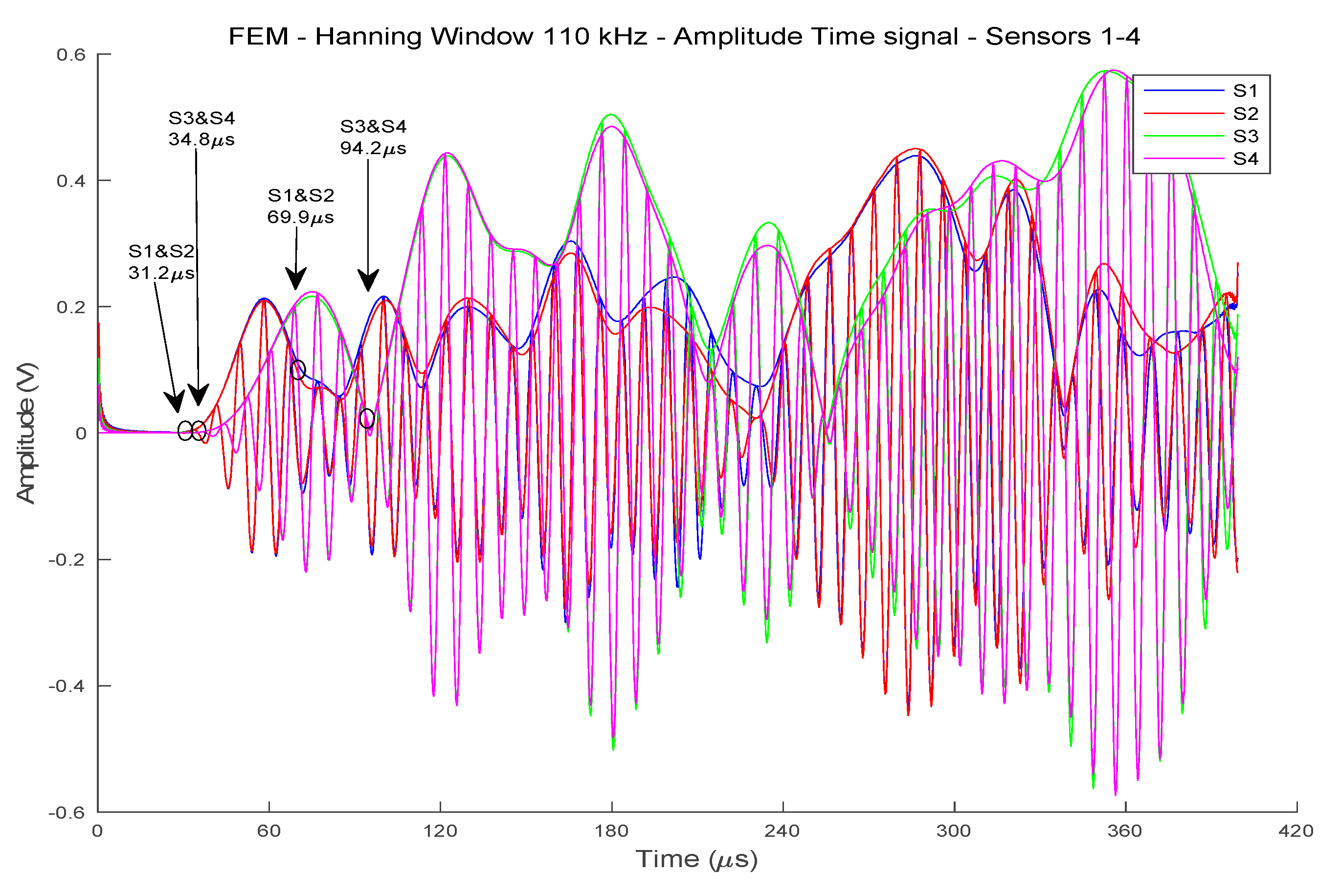
A five cycle Hanning window sinusoidal signal at that central frequency of 110 kHz was transmitted from the center of the C-Channel and received by four sensors, locations of which are shown in Figure 7. Selecting a narrowband excitation for the FEM, instead of the common waveforms found in literature, such as cosine bell, linear ramp or PLB model [44], eases the interpretation of the phase analysis for the determination of the wave modes S0 and A0 propagating through the complex structure, without compromising the functionality of this approximation.
The responses to this excitation are shown in Figure 12.
It can be observed that the signals received at sensors 1 and 2 are very similar, and so are signals at Sensors 3 and 4. This is due to the symmetry of the propagation paths for the FEM.
From the phase analysis, the ToA of S0 and A0 modes were determined and are shown in Figure 13.
The velocities obtained from these results are tabulated in Table 8 for S0 and A0 modes. The distances considered for the calculations were 150 mm from the actuator to Sensors 1 and 2, and 183 mm from actuator to Sensors 3 and 4.
6. Discussion
Acoustic emission source location requires accurate wave velocity, which is calculated through the Time of Arrival (ToA) of the propagating Lamb wave in thin structures. ToA extraction methods based on amplitude threshold may become insufficient when the amplitude of the signal captured by the transducers changes with frequency. The multimodal and dispersive nature of Lamb waves implies that the propagation of several waveforms is simultaneous, where each of them travels at different velocities. The number of modes excited depends on the frequency of the excitation; for lower frequency below the cut-off frequency, S0 and A0 modes are excited, which are used for most practical purposes. In addition, constructive and destructive interference may influence the amplitude of the signal. In which case an accurate identification of the modes, regardless of the amplitude, is required.
Many studies found in the literature strategically place the sensor such that sufficient propagation distance and difference in modes velocities can take place. These studies are usually set up on flat panels allowing for different waveform modes to separate, such that the starting and ending instants of each mode are relatively simple to determine. In this situation, methods based on amplitude threshold can be applied, provided that the wave modes are well separated, and the received waveform has high Signal to Noise Ratio (SNR). However, the behavior of Lamb waves propagating in structures with complex geometry is known to create overlapping waveforms either with reflections from the boundaries or between modes. In some cases, the low SNR of the amplitude in the time domain signal may not be sufficient to determine the correct wave mode and its ToA.
The phase analysis of the signal obtained from the Hilbert Transform (HT) proposed in this study provides a means for mode identification and ToA extraction from the sudden variations of signal’s phase, independently of the amplitude of the signal. This variation is the transition between steady deviations of phase with time; or else from an invariant phase, corresponding to null energy transportation, or from a random fluctuating noise phase, to a steady variation of phase with time. This corresponds to the dominant frequency band, as shown in Figure 11, from PLB; or almost constant phase variation, as fC or central frequency, if the waveform is a narrowband wave, as shown in Figure 13, from FEM fC = 110 kHz. In the case of the PLB signal, which is broadband in nature, the phase shows a steady but not constant increase with time. This variation of phase with time takes its maximum value upon wave arrival, gradually getting lower due to a decrease of instantaneous frequency with time, caused by the dispersive nature of Lamb waves. The frequency content of the wave arriving at the sensor changes, i.e., higher frequencies propagate faster than lower frequencies. This dispersive effect is also observed in Figure 11. In the case of the FEM, the phase variation is constant, at a rate corresponding to the central frequency fC.
The initial results on the use of AE for locating a hidden fatigue crack in the same structure analyzed in this study were presented in [43]. In this initial study, the A0 speed for damage identification was used; however, at the time it was unknown to the authors, which mode of the wave was actually being utilized. The initial estimate on damage location, which assumed the S0 wave, was incorrect, showing damage emanating from a wrong hole in the blind test on the C-Channel. In a second attempt and due to failing to find the hidden emanating crack, the authors made use of the lower speed (A0 speed), which successfully located the damage hole on the C-Channel. However, this guessing between the use of the S0 or A0 speed led the researchers to formulate a method that would provide a greater level of confidence on the actual mode being used to trigger the AE system for a specific threshold setting.
Table 9 summarizes the results obtained in the present study, for AST, PLB and the FEM using amplitude threshold and phase analysis method.
The ToA determined from the AST signal and analyzed using the amplitude threshold technique produced an average wave velocity of 2691 m/s, while the PLB test produced a velocity of 5319 m/s. The difference in the wave velocity could lead to questioning on which velocity should be used for damage location, as both methods (AST and PLB) are commonly used for wave speed calibration in AE.
The phase analysis of the PLB results revealed the velocity of propagation of S0 mode, averaging 6135 m/s considering the results from both PLB locations. Due to the complex geometry and the broadband signals propagation, multiple reflections and high level of dispersion generate additional phase abrupt variations before the A0 mode arrival. Therefore, the wave velocity obtained from the AST tests is taken as an initial approximation value for the A0 mode velocity. The phase analysis of the PLB results with this velocity as initial value, suggested an average velocity of 2757 m/s for mode A0.
The combination of these results and the threshold-based results from AST and PLB led to conclude that the PLB test captured the S0 velocity, while the AST obtained the A0 velocity, as a consequence of the selected amplitude threshold, the capability of the sensors used to capture the S0 and the A0 wave modes, and the differences in amplitude characteristics between a PLB and AST; thus, leading to different values of ToA as two different modes are being identified.
The difference in velocity of mode A0 from AST threshold method and from PLB phase analysis may be due to the different excitation method in each case, as AST and PLB in general excite different frequencies. Thereby the velocity of propagation of the waves excited in the AST test is different in general from the velocity in the PLB test.
The FEM made use of a Hanning window at 110 kHz central frequency provided by the FFT of the PLB tests. A Hanning window with the same dominant frequency was selected instead of a wideband frequency more representative of the PLB signal, in order to simplify the wave propagation analysis needed for the determination of the ToA of mode A0 in the present wing-box structure. The difference in the nature of the signals between a PLB and a Hanning window could explain the error margin in the computed ToA for the two signals, which from the results in Table 9 showed a maximum of 26%. It was never the intention of the authors to suggest that the model was detailed enough or sufficiently refined to accurately simulate the complex wave propagation behavior of such a large and complex structure. The authors believe that a 26% margin of error, although far from perfect, is still reasonable considering the: (i) complex nature of the structure in question; (ii) the assumptions made by FEM in which all the parts are perfectly attached; (iii) the shell theory approximation used to model the composite skin; (iv) the lack of an attenuation model, just to name a few. In addition, one of the challenges presented in simulating Lamb wave propagation in large complex structure is the computational cost and time required to obtain a solution within a reasonable amount of time. Nevertheless, the simulation results provided a means for visualization of the wave propagating through a complex structure, allowing the researchers to make sense of the newly developed technique for wave modes identification which despite all the deficiencies and assumptions, was shown to be able to determine the correct identification of the S0 and A0 wave modes in both an experimental setting and in a coarse FEM.
One interesting aspect observed through this model, was that although wave propagation in composite materials is known to have a non-circular wave propagation velocity front, when the composite layup is symmetrical and thick (36 plies), the wave traveled as if the material had a behavior close to isotropic. In addition, the methodology for wave mode identification was shown to be effective and repeatable in both the experiment and the model.
The identification of the accurate ToA of the signal is critical in determining the correct location of the acoustic emission source. In flat plate experiments like the ones that are typically found in the literature, one is able to measure very precisely the ToA, as the direct paths between two sensors are known. However, in complex structures finding the direct path can be challenging. In spite of the more accurate determination of the ToA, the accuracy of the calculation of the wave velocity depends on the propagation distance. Wave velocity of propagation in a complex structure is obtained from the assumption of a specific propagation path in the 3D structure, in order to obtain an average velocity value along this path. This average depends on geometry and material of the different parts of the structure, which in general can also be different for each propagation path. Therefore, the distances considered for the estimation of the wave velocity also influence the accuracy of its calculation.
7. Conclusions
The novel approach presented in this study makes use of the Hilbert Transform for the calculation of the phase and instantaneous frequency responses of both experimental and numerical signals, for the identification of the propagated modes, and the determination of their ToA. The technique presented here demonstrated that a wave packet with a predominant central frequency (fC), excited using a Hanning window, can be detected by a phase abrupt variation. In addition, it was shown that changes in phase and instantaneous frequency of Lamb wave signals can be used for detecting and identifying individual Lamb wave mode packets even in signals containing broadband frequencies. The technique is capable of accurately identifying the arrival of S0 mode. For the identification of the A0 mode from the broadband signals in complex structures, the phase analysis gets more complex, but with the aid of an approximation value given by a second experimental test (AST), which was validated with numerical simulation (FEM), and analytical dispersion curves calculation, the A0 mode arrival can be determined more accurately. The use of central frequency packets (Hanning window) for simulating Lamb wave propagation in a complex structure through FEM served as a means of verification of the presented wave mode extraction approach presented in this paper. The use of ABAQUS CAETM, and the computational costs are still excessive for large detailed simulations for real-life applications, thus the needs for the analytical approach described in this manuscript for proper selection of wave mode and velocity for the location algorithms.
The accuracy in the calculation of the wave velocity in a complex structure depends on the propagation distances considered for such calculation, which depend on the propagation path assumed for the specific wave being analyzed. The resulting velocity is only an average value of the velocities in each structural part along this propagation path. The methodology based on a combination of HT Phase analysis and Instantaneous frequency of the signal has shown that the wave speed for the S0 and A0 modes can be obtained with a margin of error between 15% and 3% respectively. This process has been shown to operate in a complex structure such as a wingbox and validated through three different tests signals (AST, PLB and Hanning Window).
Author Contributions
Conceptualization, M.B.-R. and M.M.; Data curation, M.B.-R. and D.G.; Formal analysis, M.B.-R. and M.M.; Funding acquisition, M.M.; Investigation, D.G. and S.P.; Methodology, M.B.-R.; Project administration, M.M.; Resources, S.P. and M.M.; Software, M.B.-R., S.P. and M.M.; Supervision, M.M.; Visualization, M.B.-R. and M.M.; Writing – original draft, M.B.-R.; Writing – review & editing, M.B.-R., S.P. and M.M.
Funding
This research was partially funded by Defence Research and Development Canada.
Acknowledgments
The authors would like to thank: Delft University of Technology for the financial support; Marko Yanishevsky and Michael Brothers from the National Research Council of Canada for their technical support and advice; Phil Irving and Peter Foote from Cranfield University for their support and advice; Bruno Rocha from Algonquin College for his support and advice; and NVIDIA Corporation for their donation of a TESLA K40 GPU hardware card to the Holistic Structural Integrity Process Laboratory at Clarkson University.
Conflicts of Interest
The authors declare no conflict of interest.
References
- Gagar, D.O.; Foote, P.D.; Irving, P.E. Effects of loading and sample geometry on acoustic emission generation during fatigue crack growth: Implications for structural health monitoring. Int. J. Fatigue 2015, 81, 117–127. [Google Scholar] [CrossRef]
- Daniel, I.M.; Luo, J.J.; Sifniotopoulos, C.G.; Chun, H.J. Acoustic emission monitoring of fatigue damage in metals. NDT&E 1998, 14, 71–87. [Google Scholar]
- Scruby, C.B.; Baldwin, G.R.; Stacey, K.A. Characterization of fatigue crack extension by quantitative acoustic emission. Int. J. Fract. 1985, 28, 201–222. [Google Scholar]
- Moorthy, V.; Jayakumar, T.; Raj, B. Influence of microstructure on acoustic emission behavior during stage 2 fatigue crack growth in solution annealed, thermally aged and weld specimens of AISI type 316 stainless steel. Mater. Sci. Eng. A 1996, 212, 273–280. [Google Scholar] [CrossRef]
- Lindley, T.C.; Palmer, I.G.; Richards, C.E. Acoustic emission monitoring of fatigue crack growth. Mater. Sci. Eng. 1978, 32, 1–15. [Google Scholar] [CrossRef]
- Holford, K.M. Acoustic emission-basic principles and future directions. Strain 2000, 36, 51–54. [Google Scholar] [CrossRef]
- Meriaux, J.; Boinet, M.; Fouvry, S.; Lenain, J.C. Identification of fretting fatigue crack propagation mechanisms using acoustic emission. Tribol. Int. 2010, 43, 2166–2174. [Google Scholar] [CrossRef]
- Reifsnider, K.L.; Schulte, K.; Duke, J.C. Long-term fatigue behavior of composite materials. In STP813-EB Long-Term Behavior of Composite; O’brien, T.K., Ed.; ASTM International: West Conshohocken, PA, USA, 1983; Volume ASTM STP 8, pp. 136–159. [Google Scholar] [CrossRef]
- Pant, S.; Laliberte, J.; Martinez, M.; Rocha, B.; Ancrum, D. Effects of composite lamina properties on fundamental Lamb wave mode dispersion characteristics. Compos. Struct. 2015, 124, 236–252. [Google Scholar] [CrossRef]
- Moser, F.; Jacobs, L.J.; Qu, J. Modeling elastic wave propagation in waveguides with the finite element method. NDT&E Int. 1999, 32, 225–234. [Google Scholar] [CrossRef]
- Memmolo, V.; Boffa, N.D.; Maio, L.; Monaco, E.; Ricci, F. Damage localization in composite structures using a guided waves based multi-parameter approach. Aerospace 2018, 5, 111. [Google Scholar] [CrossRef]
- Ochôa, P.; Groves, R.M.; Benedictus, R. Systematic multiparameter design methodology for an ultrasonic health monitoring system for full-scale composite aircraft primary structures. Struct. Control Health Monit. 2019, 26, 2340. [Google Scholar] [CrossRef]
- Wu, Z.; Gao, D.; Wang, Y.; Rahim, G. In-service structural health monitoring of a full-scale composite horizontal tail. J. Wuhan Univ. Technol.-Mater. Sci. Ed. 2015, 30, 1215–1224. [Google Scholar] [CrossRef]
- Gao, D.; Wang, Y.; Wu, Z.; Rahim, G. Structural health monitoring technology for a full-scale aircraft structure under changing temperature. Aeronaut. J. 2014, 118, 1519–1537. [Google Scholar] [CrossRef]
- Zhao, X.; Gao, H.; Zhang, G.; Ayhan, B.; Yan, F.; Kwan, C.; Rose, J.L. Active health monitoring of an aircraft wing with embedded piezoelectric sensor/actuator network: I. Defect detection, localization and growth monitoring. Smart Mater. Struct. 2007, 16, 1208–1217. [Google Scholar] [CrossRef]
- Ge, M. Analysis of source location algorithms, part 1: Overview and non-iterative methods. J. Acoust. Emiss. 2003, 21, 29–51. [Google Scholar]
- Gresil, M.; Giurgiutiu, V. Prediction of attenuated guided waves propagation in carbon fiber composites using Rayleigh damping model. J. Intell. Mater. Syst. Struct. 2014, 26, 2151–2169. [Google Scholar] [CrossRef]
- Wilcox, P.D. A rapid signal processing technique to remove the effect of dispersion from guided wave signals. IEEE Trans. Ultrason. Ferroelectr. Freq. Control 2003, 50, 419–427. [Google Scholar] [CrossRef]
- Pant, S.; Laliberte, J.; Martinez, M.; Rocha, B. Derivation and experimental validation of Lamb wave equations for an n-layered anisotropic composite laminate. Compos. Struct. 2014, 111, 566–579. [Google Scholar] [CrossRef]
- Martinez, M.; Pant, S.; Yanishevsky, M.; Backman, D. Residual stress effects of a fatigue crack on guided Lamb waves. Smart Mater. Struct. 2017, 26, 115004. [Google Scholar] [CrossRef]
- Ge, M.; Zhang, G.C.; Du, R.; Xu, Y. Feature Extraction from Energy Distribution of Stamping Processes Using Wavelet Transform. J. Vib. Control Modal Anal. 2002, 8, 1023–1032. [Google Scholar] [CrossRef]
- Masurkar, F.A.; Yelve, N.P. Lamb Wave Based Experimental and Finite Element Simulation Studies for Damage Detection in an Aluminum and a Composite Plate using Geodesic Algorithm. Int. J. Acoust. Vib. 2017, 22, 413–421. [Google Scholar] [CrossRef]
- Marc, N.; Laurence, J.J.; Jianmin, Q.; Jacek, J. Time-frequency representations of Lamb waves. J. Acoust. Soc. Am. 2001, 109, 1841. [Google Scholar] [CrossRef]
- Gao, W.; Glorieux, C.; Thoen, J. Laser ultrasonic study of Lamb waves: Determination of the thickness and velocities of a thin plate. Int. J. Eng. Sci. 2003, 41, 219–228. [Google Scholar] [CrossRef]
- Baxter, M.G.; Pullin, R.; Holford, K.M.; Evans, S.L. Delta T source location for acoustic emission. Mech. Syst. Signal Process. 2007, 21, 1512–1520. [Google Scholar] [CrossRef]
- Haider, M.F.; Giurgiutiu, V. Analysis of axis symmetric circular crested elastic wave generated during crack propagation in a plate: A Helmholtz potential technique. Int. J. Solids Struct. 2018, 134, 130–150. [Google Scholar] [CrossRef]
- AMSY-6 Handbook; Vallen System GmbH: Schäftlarner, Germany, October 2015.
- Martinez, M.; Rocha, B.; Li, M.; Shi, G.; Beltempo, A.; Rutledge, R.S.; Yanishevsky, M. Load monitoring of aerospace structures utilizing micro-electro-mechanical systems for static and quasi-static loading conditions. Smart Mater. Struct. 2012, 21, 115001. [Google Scholar] [CrossRef]
- Greve, D.W.; Neumann, J.J.; Nieuwenhuis, J.H.; Oppenheim, I.J.; Tyson, N.L. Use of Lamb Waves to Monitor Plates: Experiments and Simulations. In Proceedings of the SPIE 5765 Smart Structures and Materials Sensors and Smart Structures Technologies for Civil, Mechanical, and Aerospace Systems, San Diego, CA, USA, 17 May 2005. [Google Scholar] [CrossRef]
- Soden, P.D.; Hinton, M.J.; Kaddour, A.S. Lamina Properties, Lay-Up Configurations and Loading Conditions for a Range of Fibre-Reinforced Composite Laminates. Compos. Sci. Technol. 1998, 58, 1011–1022. [Google Scholar] [CrossRef]
- American Society of Composites. Tenth Technical Conference; CRC Press: Boca Raton, FA, USA, 17 October 1995; ISBN 1566763762. [Google Scholar]
- WD Sensor. Available online: http://www.physicalacoustics.com/content/literature/sensors/Model_WD.pdf (accessed on 20 May 2019).
- PCI-2—PCI-Based Two-Channel AE Board & System. Available online: https://www.physicalacoustics.com/by-product/pci-2/ (accessed on 20 May 2019).
- Akaike, H. Information theory and an extension of the maximum likelihood principle. In Second International Symposium on Information Theory; Akademiai Kiado: Budapest, Hungary, 1973; pp. 267–281. [Google Scholar]
- Sedlak, P.; Hirose, Y.; Enoki, M.; Sikula, J. Arrival Time Detection in Thin Multilayer Plates on the Basis of Akaike Information Criterion. J. Acoust. Emiss. 2008, 26, 182–188. [Google Scholar]
- David, I.J. The Industrial Electronics Handbook; Technology & Engineering; CRC Press: Boca Raton, FA, USA, 1997; p. 743. [Google Scholar]
- Bai, F.; Gagar, D.; Foote, P.; Zhao, Y. Comparison of alternatives to amplitude thresholding for onset detection of acoustic emission signals. Mech. Syst. Signal Process. 2017, 84, 717–730. [Google Scholar] [CrossRef]
- Cohen, L. Time-Frequency Analysis; Prentice Hall Signal Processing Series; Prentice-Hall: Upper Saddle River, NJ, USA, 1995. [Google Scholar]
- R15I-AST—150 kHz Integral Preamp AE Sensor. Available online: http://www.physicalacoustics.com/by-product/sensors/R15I-AST-150-kHz-Integral-Preamp-AE-Sensor (accessed on 4 February 2018).
- Erturk, A.; Inman, D. Piezoelectric Energy Harvesting; John Wiley and Sons Ltd.: Hoboken, NJ, USA, 2011; ISBN 978-0-470-68254-8. [Google Scholar]
- Boon, M.J.G.N. Temperature and Load Effects in Modelling and Experimental Verification of Acoustic Emission Signals for Structural Health Monitoring Applications, Faculty of Aerospace Engineering. Master’s Thesis, Delft University of Technology, Delft, The Netherlands, 2014. [Google Scholar]
- Chen, L.; Dong, Y.; Meng, Q.; Liang, W. FEM simulation for Lamb Wave evaluate the defects of plates. In Proceedings of the Microwave and Millimeter Wave Circuits and Systems Technologies (MMWCST), Chengdu, China, 19–20 April 2012. [Google Scholar]
- Gagar, D.; Martinez, M.; Yanishevsky, M.; Rocha, B.; McFeat, J.; Foote, P.; Irving, P. Detecting and Locating Fatigue Cracks in a Complex Wing-Box Structures using the Acoustic Emission Technique: A Verification Study. In Proceedings of the 9th 2013 International Workshop on Structural Health Monitoring, Stanford, CA, USA, 10–12 September 2013; DEStech Publications, Inc.: Stanford, CA, USA, 2013; pp. 65–72. [Google Scholar]
- Sause, M.G. Investigation of pencil-lead breaks as acoustic emission sources. J. Acoust. Emiss. 2011, 29, 184–196. [Google Scholar]
Figure 1.
The National Research Council Canada Structural Health Monitoring (NRC SHM) wing-box test rig.
Figure 1.
The National Research Council Canada Structural Health Monitoring (NRC SHM) wing-box test rig.

Figure 2.
Sensor location and overall depiction of their placement, within the structure and with respect to the 15 holes locations.
Figure 2.
Sensor location and overall depiction of their placement, within the structure and with respect to the 15 holes locations.

Figure 3.
Mode identification process.

Figure 4.
(a) Time signal of three waves at different frequencies; (b) Phase of the same three waves; (c) Instantaneous frequency of the three waves. The arrival instants of the waveforms are represented by the red dots.
Figure 4.
(a) Time signal of three waves at different frequencies; (b) Phase of the same three waves; (c) Instantaneous frequency of the three waves. The arrival instants of the waveforms are represented by the red dots.

Figure 5.
(a) Waveform, phase and instantaneous frequency of two overlapping signals, with different central frequencies, 50 and 150 kHz. (b) Magnified view of instant (1), arrival of wave packet at frequency 50 kHz. (c) Frequency content of the signal showing the two central frequencies.
Figure 5.
(a) Waveform, phase and instantaneous frequency of two overlapping signals, with different central frequencies, 50 and 150 kHz. (b) Magnified view of instant (1), arrival of wave packet at frequency 50 kHz. (c) Frequency content of the signal showing the two central frequencies.

Figure 6.
Flowchart of the process for modes identification with phase analysis. VS0, velocity of mode S0; v’A0 corrected approximation to velocity of mode A0 for complex structures and broadband signals.
Figure 6.
Flowchart of the process for modes identification with phase analysis. VS0, velocity of mode S0; v’A0 corrected approximation to velocity of mode A0 for complex structures and broadband signals.

Figure 7.
Simplified Finite Element Model (FEM) of the mid-section of the wing-box.

Figure 8.
Results from the Pencil Lead Break (PLB) performed at hole 3 (H3) received at Sensors S1, S2, S3 and S4. (a) Shows the amplitude of the signals while (b) is the frequency spectrum, normalized to the maximum amplitude for each sensor.
Figure 8.
Results from the Pencil Lead Break (PLB) performed at hole 3 (H3) received at Sensors S1, S2, S3 and S4. (a) Shows the amplitude of the signals while (b) is the frequency spectrum, normalized to the maximum amplitude for each sensor.

Figure 9.
Response signal and threshold line at 45 dB at Sensors 1 (green) and Sensor 2 (pink), from the PLB at hole 4. In blue is the indication of the ToA given by the amplitude threshold method.
Figure 9.
Response signal and threshold line at 45 dB at Sensors 1 (green) and Sensor 2 (pink), from the PLB at hole 4. In blue is the indication of the ToA given by the amplitude threshold method.

Figure 10.
Flowchart of the process for modes identification with phase analysis of the PLB signals. VS0, velocity of mode S0; VAST, wave velocity provided by the AST threshold-test, and validated by phase analysis and DCs as VA0; VPLB, wave velocity provided by the PLB threshold-test, and validated by phase analysis and DCs as VS0; dAST and dPLB, effective distance for the propagation path in AST and PLB test respectively.

Figure 11.
Phase and instantaneous frequency responses at Sensor 1 (green) and Sensor 2 (pink), from the PLB at hole 4. The ToA given by the phase analysis method is indicated for modes S0 (blue) and A0 (red).
Figure 11.
Phase and instantaneous frequency responses at Sensor 1 (green) and Sensor 2 (pink), from the PLB at hole 4. The ToA given by the phase analysis method is indicated for modes S0 (blue) and A0 (red).

Figure 12.
Amplitude response, and envelope of the signals at Sensors 1, 2, 3 and 4, showing ToA of modes S0 and A0 given by the phase analysis.
Figure 12.
Amplitude response, and envelope of the signals at Sensors 1, 2, 3 and 4, showing ToA of modes S0 and A0 given by the phase analysis.

Figure 13.
Phase and instantaneous frequency response at Sensors 1, 2, 3, and 4 with an indication of the ToA of S0 and A0 modes given by the phase analysis.
Figure 13.
Phase and instantaneous frequency response at Sensors 1, 2, 3, and 4 with an indication of the ToA of S0 and A0 modes given by the phase analysis.


Table 1.
Material properties of the Carbon Fiber Reinforced Polymer (CFRP) skins.
| E11 | E22 | υ12 | G12 | G13 | G23 | ρ |
|---|---|---|---|---|---|---|
| 128 GPa | 13 GPa | 0.3 | 5.86 GPa | 6.1 GPa | 3.6 GPa | 1265 kg/m3 |
Table 2.
Location of fasteners and sensors—distances from tip to root.
| Fastener Hole | Longitudinal Position on Spar (mm) | Fastener Hole | Longitudinal Position on Spar (mm) | Sensor | Longitudinal Position on Spar (mm) |
|---|---|---|---|---|---|
| Hole 3 | 70.8 | Hole 9 | 223.2 | Sensor 1 | 347.0 |
| Hole 4 | 96.2 | Hole 10 | 248.6 | Sensor 2 | 60.0 |
| Hole 5 | 121.6 | Hole 11 | 274.0 | Sensor 3 | 347.0 |
| Hole 6 | 147.0 | Hole 12 | 299.4 | Sensor 4 | 60.0 |
| Hole 7 | 172.4 | Hole 13 | 324.8 | ||
| Hole 8 | 197.8 |
| Orthotropic Material Properties (GPa) | ||||||
|---|---|---|---|---|---|---|
| D1111= D2222 | D1122 | D1133= D2233 | D3333 | D1212= D1313 | D2323 | |
| 132 | 87.6 | 73.4 | 162 | 43.7 | 22.4 | |
| Piezoelectric Charge Constants (10−12C/N) | Relative Dielectric Constants | |||||
| d31 | d33 | d15 | k11= k22 | k33 | εo (10−12F/m) | |
| −125 | 290 | 480 | 1943 | 1897 | 8.854 | |
| Thickness (mm) | Diameter (mm) | Density (kg/m3) | Type of Element | |||
| 6.5 | 20 | 7850 | C3D8E | |||
Table 4.
Velocity range of modes S0 and A0, for the frequency range of interest: 30–350 kHZ.
| Material | VA0 Range | VA0 110 kHz | VS0 Range | VS0 110 kHz |
|---|---|---|---|---|
| AA 7075 | 1175–2610 | 1950 | 5340–4995 | 5335 |
| CFRP | 1445–3542 | 2400 | 7790–7655 | 7705 |
Table 5.
Automatic Sensor Test (AST) wave velocity calibration on the wing-box structure, Sensors 1–4 located on the C-channel spar and adjacent spar respectively; distance between sensor pairs dAST = 287mm.
Table 5.
Automatic Sensor Test (AST) wave velocity calibration on the wing-box structure, Sensors 1–4 located on the C-channel spar and adjacent spar respectively; distance between sensor pairs dAST = 287mm.
| Number of Events | Time Interval between Sensors [µs] | Velocity [m/s] |
|---|---|---|
| 50 | ∆t (1,2) 105 | 2733.3 |
| 50 | ∆t (2,1) 103 | 2786.4 |
| 50 | ∆t (3,4) 118 | 2432.2 |
| 50 | ∆t (4,3) 102 | 2813.7 |
| Average | 2691.4 | |
Table 6.
Wave velocity calibration on the assembled wing-box structure—Sensors 1–2 located on the C-channel spar; distance between sensor pairs d = 287 mm.
Table 6.
Wave velocity calibration on the assembled wing-box structure—Sensors 1–2 located on the C-channel spar; distance between sensor pairs d = 287 mm.
| PLB at Fastener Hole 3—10.8 mm from Sensor 2; dPLB = 265.4 mm | ||
|---|---|---|
| Event Number | Time Interval between Sensors 1 and 2 [µs] | Velocity [m/s] |
| 1 | ∆t(1,2) 51.0 | 5203.9 |
| 2 | ∆t(1,2) 49.2 | 5394.3 |
| 3 | ∆t(1,2) 50.0 | 5308.0 |
| 4 | ∆t(1,2) 48.0 | 5529.2 |
| Average | 5358.9 | |
| PLB at Fastener Hole 4—32.6 mm from Sensor 2; dPLB = 214.6 mm | ||
| Event Number | Time Interval between Sensors 1 and 2 [µs] | Velocity [m/s] |
| 1 | ∆t(1,2) 40.0 | 5365.0 |
| 2 | ∆t(1,2) 41.6 | 5158.7 |
| 3 | ∆t(1,2) 42.5 | 5049.4 |
| 4 | ∆t(1,2) 38.7 | 5545.2 |
| Average | 5279.6 | |
Table 7.
S0 and A0 velocities using phase analysis on experimental PLB.
| PLB at Fastener Hole 3. Velocity Measured from Phase Discontinuities. dPLB = 265.4 mm | ||
|---|---|---|
| Event Number | Velocity Measured [m/s] | |
| Mode S0 | Mode A0 | |
| 1 | 6349 | 2811 |
| 2 | 6201 | 2969 |
| 3 | 6319 | 2686 |
| 4 | 6059 | 2770 |
| Average | 6232 | 2809 |
| PLB at Fastener Hole 4. Velocity Measured from Phase Discontinuities. dPLB = 214.6 mm | ||
| Event Number | Velocity Measured [m/s] | |
| Mode S0 | Mode A0 | |
| 1 | 6167 | 2676 |
| 2 | 5961 | 2730 |
| 3 | 5928 | 2716 |
| 4 | 6097 | 2696 |
| Average | 6038 | 2705 |
Table 8.
S0 and A0 velocities using phase analysis on FEM results.
| FEM—Hanning Window at 110 kHz. Velocity Measured from Phase Discontinuities | |||
|---|---|---|---|
| Velocity Measured [m/s] | |||
| Sensors | d [mm] | Mode S0 | Mode A0 |
| 1&2 | 150 | 4812 | 2148 |
| 3&4 | 183 | 5230 | 1932 |
| Average | 5021 | 2040 | |
Table 9.
Velocity extraction summary.
| Test | Method Description | Velocity [m/s] | |
|---|---|---|---|
| AST | Amplitude Threshold | 2691 | |
| PLB at hole 3/4 | Amplitude Threshold | 5319 | |
| PLB at hole 3/4 | Phase analysis | A0 | 2757 |
| S0 | 6135 | ||
| FEM at 110kHz—Hanning Window | Phase analysis | A0 | 2040 |
| S0 | 5021 | ||
© 2019 by the authors. Licensee MDPI, Basel, Switzerland. This article is an open access article distributed under the terms and conditions of the Creative Commons Attribution (CC BY) license (http://creativecommons.org/licenses/by/4.0/).
Share and Cite
MDPI and ACS Style
Barroso-Romero, M.; Gagar, D.; Pant, S.; Martinez, M. Wave Mode Identification of Acoustic Emission Signals Using Phase Analysis. Acoustics 2019, 1, 450-472. https://doi.org/10.3390/acoustics1020026
AMA Style
Barroso-Romero M, Gagar D, Pant S, Martinez M. Wave Mode Identification of Acoustic Emission Signals Using Phase Analysis. Acoustics. 2019; 1(2):450-472. https://doi.org/10.3390/acoustics1020026
Chicago/Turabian StyleBarroso-Romero, Maria, Daniel Gagar, Shashank Pant, and Marcias Martinez. 2019. "Wave Mode Identification of Acoustic Emission Signals Using Phase Analysis" Acoustics 1, no. 2: 450-472. https://doi.org/10.3390/acoustics1020026