Article

A High-Frequency Model of a Circular Beam with a T-Shaped Cross Section

Naval Undersea Warfare Center, Newport, RI 02841, USA
*
Author to whom correspondence should be addressed.
Acoustics 2019, 1(1), 295-336; https://doi.org/10.3390/acoustics1010017
Submission received: 14 January 2019 / Revised: 8 March 2019 / Accepted: 11 March 2019 / Published: 15 March 2019

Abstract

:
This paper derives an analytical model of a circular beam with a T-shaped cross section for use in the high-frequency range, defined here as approximately 1 to 50 kHz. The T-shaped cross section is composed of an outer web and an inner flange. The web in-plane motion is modeled with two-dimensional elasticity equations of motion, and the left portion and right portion of the flange are modeled separately with Timoshenko shell equations. The differential equations are solved with unknown wave propagation coefficients multiplied by Bessel and exponential spatial domain functions. These are inserted into constraint and equilibrium equations at the intersection of the web and flange and into boundary conditions at the edges of the system. Two separate cases are formulated: structural axisymmetric motion and structural non-axisymmetric motion and these results are added together for the total solution. The axisymmetric case produces 14 linear algebraic equations and the non-axisymmetric case produces 24 linear algebraic equations. These are solved to yield the wave propagation coefficients, and this gives a corresponding solution to the displacement field in the radial and tangential directions. The dynamics of the longitudinal direction are discussed but are not solved in this paper. An example problem is formulated and compared to solutions from fully elastic finite element modeling. It is shown that the accurate frequency range of this new model compares very favorably to finite element analysis up to 47 kHz. This new analytical model is about four magnitudes faster in computation time than the corresponding finite element models.

1. Introduction

The work derived herein is a direct extension of a previous effort [1,2], that modeled the dynamics of a circular T-beam. These models accurately captured the physics of the beam up to about 8 kilohertz (kHz) for the example problem studied. The previous beam model became inaccurate above 8 kHz because of the limitations of the model’s flange component, which was a three-dimensional Donnell [3] shell formulation. The assumptions of the Donnell shell formulation typically produce model results that are too stiff, especially as frequency increases. In the new model derived here, the Donnell shell formulation is replaced with a Timoshenko-type shell formulation [4], which includes shear deformation and rotary inertia terms, resulting in a higher-frequency range of analysis. This work develops an analytical model of a circular T-shaped beam and extends the frequency range of this system compared to previous modeling efforts. It is primarily intended for use in models that have reinforced cylindrical shells that need improved accuracy at higher frequencies. These typically consist of: (1) target strength models of reinforced cylindrical structures which are applicable to active sonar target discrimination, and/or (2) hull dynamic response models which are applicable to flank array self-noise performance.
Beams are structural elements that are designed to reinforce objects against external forces. In general, they are designed to resist loads that are normal to their neutral axis. Most T-shaped beams consist of two parts, namely, the web which has one end attached to the object and the flange which is attached to the other end of the web. Bernoulli and Euler [5] derived the first accurate beam model in Cartesian coordinates and this model was extended to cylindrical coordinates. This theory uses the assumption that all sections rotate orthogonal to the neutral axis of the beam. Timoshenko [6] revised this work so that the rotation angle of the neutral axis of the beam was a function of the polar inertia and shear force. Higher order displacement functions have been added to beam theory, notably by Bickford [7] who used a third-order polynomial through the thickness of the beam to model the in-plane displacement field and Karama, Afaq and Mistou [8] who used an exponential function to model the shear distribution in the beam. These higher order models, while accurate at somewhat higher frequencies than the Timoshenko beam model, are still lumped parameter models.
Ambati [9] analyzed and discussed the in-plane response of annular rings using elasticity theory. Kirkhope [10] derived the stiffness and inertia matrices for thick circular rings using an energy method. Hawkings [11] developed a theory of inextensional vibrations of a circular ring where the principal axes of inertia of the cross section did not lie in the ring plane. Kirkhope, Bell and Olmstead [12] analyzed the vibration of closed uniform rings with unsymmetrical cross sections. Bhimaraddi [13] developed a shear deformable theory for curved beams of constant curvature by assuming a parabolic variation for the shear strains. Lin and Lee [14] studied curved Timoshenko beams with generalized boundary conditions. The preceding references are either elastic response for a rectangular beam or lumped inertial and stiffness response for a beam of varying cross section.
A large number of papers have been written on the scattered pressure field of ribbed cylinders when subjected to plane wave excitation. Konovalyuk [15] investigated the reflection of sound from a plate with arbitrarily situated ribs. Graff, Klein and Kouyoumjian [16] analyzed mass loading on a stiffened rib. Woolley also investigated mass loading of a single rib [17] and a finite number of ribs [18] with an emphasis on the back-scattered field. Marcus and Sarkissian [19] reported on the rib resonances features in the back-scattered field of a finite length shell. Tran-Van-Nhieu [20] researched the problem with an emphasis on Bloch–Floquet wave scattering. These papers [16,17,18,19,20] have generally modeled the ribs as having lumped parameter behavior. None of them incorporate the spatial dimensions of a flange attached to a web.
In this new model, the web and flange of the T-beam are modeled independently with two-dimensional elasticity equations accounting for the in-plane web motion and Timoshenko shell equations that model the three-dimensional response of the flange. For the axisymmetric model, the connection of the web and flange are modeled using three equilibrium equations and four constraint equations and the free and forced edges of the system are modeled with seven additional force and moment equations. For the non-axisymmetric model, the connection of the web and flange are modeled using five equilibrium equations and seven constraint equations and the free and forced edges of the system are modeled with twelve additional force and moment equations. Modeling the beam in this manner allows the web and flange equations of motion to incorporate higher-order dynamic effects and this makes the overall model much more accurate at higher frequencies.

2. Methods

The system under consideration is a circular closed beam, commonly called a ring, with a T-shaped cross section. The outer narrow component is called the web and the inner wide component is called the flange. The structure is excited with continuous spatial and time harmonic excitation applied to the outer edge of the web. A schematic of this system showing the dimensions and the web coordinate system is shown in Figure 1. The web coordinate system is a function of the independent variables radial direction, angular direction and time. The model of the web has no spatial extent in the longitudinal direction. The flange coordinate system has the same orientation as the web coordinate system; however, it is a function of the independent variables angular direction, longitudinal direction, and time. The model of the flange has no spatial extent in the radial direction. The beam is symmetric about the mid plane of the web.
The problem is analytically modeled using the two-dimensional plane stress elastic equations for in-plane motions of the web and Timoshenko type shell equations for three-dimensional motion of the flange. The model can calculate motion in the radial and tangential dimensions when the beam is subjected to forcing in the radial and tangential directions. The model uses the following assumptions: (1) the excitation is at a fixed frequency and fixed circumferential node number, (2) the angle at the intersection of the web and the flange is always a right angle, (3) the material properties of the web and flange are identical, and (4) the particle motion is linear. The model is developed by analyzing the system as three separate components: the web, the left part of the flange, and the right part of the flange. These model components are then combined using equilibrium and continuity equations at the intersection of the web and flange and boundary conditions at the edges. The longitudinal motion of the web is not calculated, and this is discussed in detail later in the paper.
The equations modeling the radial and tangential (in-plane) motion of the web begin with the Navier–Cauchy [21] fully elastic equations of motion. These are reduced to two plane stress equations of motion, the first one is in the radial direction and is written as
E 1 υ 2 [ 2 w w ( r , θ , t ) r 2 + 1 r w w ( r , θ , t ) r 1 r 2 w w ( r , θ , t ) ] + E 2 ( 1 + υ ) 1 r 2 2 w w ( r , θ , t ) θ 2 E ( 3 υ ) 2 ( 1 υ 2 ) 1 r 2 v w ( r , θ , t ) θ + E 2 ( 1 υ ) 1 r 2 v w ( r , θ , t ) r θ = ρ 2 w w ( r , θ , t ) t 2
and the second one is in the tangential direction and is written as
E 1 υ 2 1 r 2 2 v w ( r , θ , t ) θ 2 + E 2 ( 1 + υ ) [ 2 v w ( r , θ , t ) r 2 + 1 r v w ( r , θ , t ) r 1 r 2 v w ( r , θ , t ) ] + E ( 3 υ ) 2 ( 1 υ 2 ) 1 r 2 w w ( r , θ , t ) θ + E 2 ( 1 υ ) 1 r 2 w w ( r , θ , t ) r θ = ρ 2 v w ( r , θ , t ) t 2
where ww(r,θ,t) is the web radial displacement, vw(r,θ,t) is the web tangential displacement, E is Young’s modulus, υ is Poisson’s ratio, ρ is density, r is radius, θ is angle, t is time and the subscript w denotes the web.
The equations modeling the three-dimensional motion of the flange are Timoshenko-type shell equations [4] that have five degrees of freedom, namely longitudinal displacement at the shell middle surface, longitudinal rotation, tangential displacement at the shell middle surface, tangential rotation, and radial displacement. The equation of motion in the longitudinal direction at the middle surface of the shell is
E p 2 u f ( θ , z , t ) z 2 + ( G h a 2 ) ( 1 + I h a 2 ) 2 u f ( θ , z , t ) θ 2 ρ h 2 u f ( θ , z , t ) t 2 + ( D a ) 2 ψ z ( θ , z , t ) z 2 ( G I a 3 ) 2 ψ z ( θ , z , t ) θ 2 ( ρ I a ) 2 ψ z ( θ , z , t ) t 2 + [ E p ( 1 + υ ) 2 a ] 2 v f ( θ , z , t ) z θ + ( υ E p a ) w f ( θ , z , t ) z = 0   ,
the equation of motion of the angle of rotation of a normal to the middle surface in the r-z cylinder plane is
( D a ) 2 u f ( θ , z , t ) z 2 ( G I a 3 ) 2 u f ( θ , z , t ) θ 2 ( ρ I a ) 2 u f ( θ , z , t ) t 2 + D 2 ψ z ( θ , z , t ) z 2 + ( G I a 2 ) 2 ψ z ( θ , z , t ) θ 2 κ G h ψ z ( θ , z , t ) ρ I 2 ψ z ( θ , z , t ) t 2 + [ D ( 1 + υ ) 2 a ] 2 ψ θ ( θ , z , t ) z θ κ G h w f ( θ , z , t ) z = 0   ,
the equation of motion in the tangential direction at the middle surface of the shell is
[ E p ( 1 + υ ) 2 a ] 2 u f ( θ , z , t ) z θ + G h 2 v f ( θ , z , t ) z 2 + ( E p a 2 + D a 4 ) 2 v f ( θ , z , t ) θ 2 ( κ G a 2 ) ( h + I a 2 ) v f ( θ , z , t ) ρ h 2 v f ( θ , z , t ) t 2 + ( G I a ) 2 ψ θ ( θ , z , t ) z 2 ( D a 3 ) 2 ψ θ ( θ , z , t ) θ 2 + ( κ G a ) ( h + I a 2 ) ψ θ ( θ , z , t ) ( ρ I a ) 2 ψ θ ( θ , z , t ) t 2 + [ E p a 2 + D a 4 + ( κ G a 2 ) ( h + I a 2 ) ] w f ( θ , z , t ) θ = 0   ,
the equation of motion of the angle of rotation of a normal to the middle surface in the r-θ cylinder plane is
[ D ( 1 + υ ) 2 a ] 2 ψ z ( θ , z , t ) z θ + ( G I a ) 2 v f ( θ , z , t ) z 2 ( D a 3 ) 2 v f ( θ , z , t ) θ 2 + ( κ G a ) ( h + I a 2 ) v f ( θ , z , t ) ( ρ I a ) 2 v f ( θ , z , t ) t 2 + G I 2 ψ θ ( θ , z , t ) z 2 + ( D a 2 ) 2 ψ θ ( θ , z , t ) θ 2 κ G ( h + I a 2 ) ψ θ ( θ , z , t ) ρ I 2 ψ θ ( θ , z , t ) t 2 + [ D a 3 ( κ G a ) ( h + I a 2 ) ] w f ( θ , z , t ) θ = 0
and the equation of motion in the radial direction anywhere in the shell is
( E p υ a ) u f ( θ , z , t ) z + κ G h ψ z ( θ , z , t ) z + [ ( κ G a 2 ) ( h + I a 2 ) ( E p a 2 + D a 4 ) ] v f ( θ , z , t ) θ + G [ D a 3 + ( κ G a ) ( h + I a 2 ) ] ψ θ ( θ , z , t ) θ + κ G h 2 w f ( θ , z , t ) z 2 + [ ( κ G a 2 ) ( h + I a 2 ) ] 2 w f ( θ , z , t ) θ 2 ( E p a 2 + D a 4 ) w f ( θ , z , t ) ρ h 2 w f ( θ , z , t ) t 2 = 0   .
In Equations (3) to (7), uf(θ,z,t) is the mid-plane shell displacement in the longitudinal direction, ψz,z,t) is the shell rotation in the longitudinal direction, vf,z,t) is the mid-plane shell displacement in the tangential direction, ψθ,z,t) is the shell rotation in the circumferential direction, wf,z,t) is the shell displacement in the radial direction, the subscript f denotes the flange, z is the longitudinal coordinate of the shell, G is the shear modulus, h is the shell thickness, a is the shell radius at the mid-plane, κ is the shear correction factor, and Ep is the plate compressional modulus and is expressed as
E p = E h ( 1 υ 2 )   ,
I is the axial moment of inertia of the cross section and is written as
I = h 3 12
and D is the plate flexural modulus expressed as
D = E h 3 12 ( 1 υ 2 )   .
Later in the paper, the subscript f will be further delineated to fl to denote the left flange and fr to denote the right flange, as these are modeled independently.
The complete solution to the web in-plane displacement field in the frequency domain is [22]
v w ( r , θ , t ) = n = 1 n = + v w ( n ) ( r , θ , t ) = n = 1 n = + V n ( r )   sin ( n θ ) exp ( i ω t )
and
w w ( r , θ , t ) = n = 0 n = + w w ( n ) ( r , θ , t ) = n = 0 n = + W n ( r )   cos ( n θ ) exp ( i ω t )
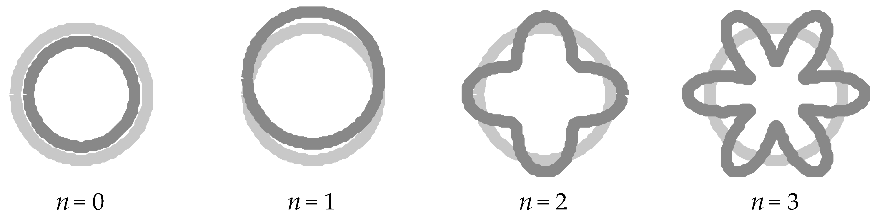
where ω is frequency, n is the circumferential node number and i is the square root of −1. Equations (11) and (12) contain all of the terms of the web solution set, i.e., the solution is complete. (Similarly, the flange solutions could also be written out as complete expansions). However, to numerically solve the problem, the component field has to be broken down into the individual axisymmetric (n = 0) and non-axisymmetric (n > 0) parts. This is accomplished below. Figure 2 is a plot of the first four circumferential n-indexed node shapes. In this figure, the undeformed shape is shown in light gray and the deformed mode shape is depicted in dark gray.
The axisymmetric solution component is now formulated. This is typically called the n = 0 solution. Because the tangential displacement components and their slopes are identically zero for this case, they need to be eliminated from the equations of motion before a problem solution is generated. Additionally, any other component differentiated with respect to the angular coordinate θ is zero and these terms are also condensed from the original equations of motion, Equations (1) to (7). Equation (1) becomes
E 1 υ 2 [ 2 w w ( r , t ) r 2 + 1 r w w ( r , t ) r 1 r 2 w w ( r , t ) ] = ρ 2 w w ( r , t ) t 2  
and the solution in the frequency domain is
w w ( 0 ) ( r , t ) = W 0 ( r ) exp ( i ω t )
where
W 0 ( r ) = C 1 ( 0 ) k p J 1 ( k p r ) C 2 ( 0 ) k p Y 1 ( k p r )
with the plate wavenumber kp equal to
k p = ω c p
and the plate wave speed cp equal to
c p = E ρ ( 1 υ 2 )  
where C1(0) and C2(0) are wave propagation constants determined below, J1 is a first-kind, first-order Bessel function, and Y1 is a second-kind, first-order Bessel function.
The flange or shell equations are reformulated for the n = 0 response, Equation (3) becomes
E p 2 u f ( z , t ) z 2 ρ h 2 u f ( z , t ) t 2 + ( D a ) 2 ψ z ( z , t ) z 2 ( ρ I a ) 2 ψ z ( z , t ) t 2 + ( υ E p a ) w f ( z , t ) z = 0   ,
and Equation (4) becomes
( D a ) 2 u f ( z , t ) z 2 ( ρ I a ) 2 u f ( z , t ) t 2 + D 2 ψ z ( z , t ) z 2 κ G h ψ z ( z , t ) ρ I 2 ψ z ( z , t ) t 2 κ G h w f ( z , t ) z = 0   .
Equations (5) and (6) are identically zero, and Equation (7) becomes
( E p υ a ) u f ( z , t ) z + κ G h ψ z ( z , t ) z + κ G h 2 w f ( z , t ) z 2 + ( E p a 2 + D a 4 ) w f ( z , t ) ρ h 2 w f ( z , t ) t 2 = 0   .
The solution set to Equations (18) to (20) on the left flange is written as [23]
u f l ( z , t ) = j = 1 j = 6 C j + 2 ( 0 ) M j ( 0 ) exp ( λ j ( 0 ) z ) exp ( i ω t )   ,
ψ f l , z ( z , t ) = j = 1 j = 6 C j + 2 ( 0 ) N j ( 0 ) exp ( λ j ( 0 ) z ) exp ( i ω t )
and
w f l ( z , t ) = j = 1 j = 6 C j + 2 ( 0 ) exp ( λ j ( 0 ) z ) exp ( i ω t )   .    
Similarly, the solution set to Equations (18) to (20) on the right flange is written as
u f r ( z , t ) = j = 1 j = 6 C j + 8 ( 0 ) M j ( 0 ) exp ( λ j ( 0 ) z ) exp ( i ω t )   ,
ψ f r , z ( z , t ) = j = 1 j = 6 C j + 8 ( 0 ) N j ( 0 ) exp ( λ j ( 0 ) z ) exp ( i ω t )
and
w f r ( z , t ) = j = 1 j = 6 C j + 8 ( 0 ) exp ( λ j ( 0 ) z ) exp ( i ω t )   .  
where λj are the spatial eigenvalues, Ci(0)’s are wave propagation constants determined below, and the terms Mj and Nj are constants that properly scale the displacement and slope variables to one another.
The solutions to the spatial eigenvalues are now determined. This begins by inserting Equations (21) to (23)—or (24) to (26)—into Equations (18) to (20), which results in the matrix
B 0 = [ E p λ 2 + h ω 2 ρ D λ 2 a + I ω 2 ρ a E p υ λ a D λ 2 a + I ω 2 ρ a D λ 2 κ G h + I ω 2 ρ κ G h λ E p υ λ a κ G h λ κ G h λ 2 + h ω 2 ρ ( D a 4 + E p a 2 ) ]   .
The eigenvalues are found by setting the determinant of B0 to zero which yields the characteristic equation
a 6 λ 6 + a 4 λ 4 + a 2 λ 2 + a 0 = 0
and solving this equation produces the six eigenvalues for the n = 0 case. The formulas for the constants a6, a4, a2 and a0 are listed in Appendix A. Once the individual i-indexed eigenvalues are known, the two constants Mi and Ni each have six i-indexed values and are solved individually by using the first two rows of Equation (27), which results in
{ M i ( 0 ) N i ( 0 ) } = [ E p ( λ i ( 0 ) ) 2 + h ω 2 ρ D ( λ i ( 0 ) ) 2 a + I ω 2 ρ a D ( λ i ( 0 ) ) 2 a + I ω 2 ρ a D ( λ i ( 0 ) ) 2 κ G h + I ω 2 ρ ] 1 { υ E p λ i ( 0 ) a κ G h λ i ( 0 ) }   .
For the axisymmetric case, three flange stress resultants are needed for the continuum balance with the web. The first is the normal force in the z direction and is written as [4]
N z z ( z ) = E p d u f ( z ) d z + D a d ψ z ( z ) d z + υ E p a w f ( z )   ,
N z z ( z ) = i = 1 i = 6 C i + 2 ( 0 ) exp ( λ i ( 0 ) z ) ( υ E p a + E p M i ( 0 ) λ i ( 0 ) + D N i ( 0 ) λ i ( 0 ) a )   ,
the second is the bending moment with respect to the z direction and is written as [4]
M z z ( z ) = D a d u f ( z ) d z + D d ψ z ( z ) d z   ,
M z z ( z ) = i = 1 i = 6 C i + 2 ( 0 ) exp ( λ i ( 0 ) z ) ( D M i ( 0 ) λ i ( 0 ) a + D N i ( 0 ) λ i ( 0 ) )
and the third is the shear force with respect to the z direction and is written as [4]
Q z ( z ) = κ G h [ ψ z ( z ) + d w f ( z ) d z ]   ,
Q z ( z ) = i = 1 i = 6 C i + 2 ( 0 ) exp ( λ i ( 0 ) z ) κ G h ( λ i ( 0 ) + N i ( 0 ) )   .
Note that in Equations (30) to (35), and all equations hereafter, the frequency harmonic terms and corresponding time dependence are implicit. The constants in Equations (31), (33), and (35) are written for the left flange. If the constants on the right flange are desired, then the term i + 2 should be replaced with i + 8. The normal radial force in the web is [16]
T r r ( w ) ( r ) = E 1 υ 2 d w w ( r ) d r +   E υ 1 υ 2 ( 1 r ) w w ( r ) ,  
T r r ( w ) ( r ) = [ E k p r ( 1 + υ ) J 1 ( k p r ) E k p 2 ( 1 υ 2 ) J 0 ( k p r ) ] C 1 ( 0 ) + [ E k p r ( 1 + υ ) Y 1 ( k p r ) E k p 2 ( 1 υ 2 ) Y 0 ( k p r ) ] C 2 ( 0 )
where J0 is a first-kind, zero-order Bessel function and Y0 is a second-kind, zero-order Bessel function.
The solution to the constants C1(0)C14(0) are found using equilibrium and continuity expressions from the system. Figure 3 is a free body diagram that shows the 14 individual generalized forces that are present on the boundaries of the system. Note that although these are called generalized forces, they all have units other than force. The boundary condition at the outer edge of the web (r = b) is
T r r ( w ) ( b ) = P 0
where P0 is the magnitude of the radial external pressure for the n = 0 axisymmetric load applied to the outer edge of the web. The three boundary conditions at the free edge of the left flange (z = zL) are
N z z ( f l ) ( z L ) = M z z ( f l ) ( z L ) = Q z ( f l ) ( z L ) = 0
where it is noted that zL < 0. Similarly, the three boundary conditions at the free edge of the right flange (z = zR) are
N z z ( f r ) ( z R ) = M z z ( f r ) ( z R ) = Q z ( f r ) ( z R ) = 0   .
There are two force balances at the intersection of the web and flange (r = a and z = 0). The force balance in the radial direction is
b w T r r ( w ) ( a ) Q z ( f l ) ( 0 ) + Q z ( f r ) ( 0 ) = 0
and the force balance in the longitudinal direction is
N z z ( f l ) ( 0 ) + N z z ( f r ) ( 0 ) = 0   .
Additionally, there is a bending moment balance at this location and this equation is
M z z ( f l ) ( 0 ) + M z z ( f r ) ( 0 ) = 0   .
There are three displacement continuity equations at the intersection of the web and the flange and these are written as
u f l ( 0 ) = u f r ( 0 )   ,
w w ( a ) = w f l ( 0 )
and
w w ( a ) = w f r ( 0 )   ,
and one slope continuity equation written as
ψ f l , z ( 0 ) = ψ f r , z ( 0 )   .
Equations (21) to (26), (30), (32), and (34) are inserted into Equations (38) to (47), and this results in an algebraic matrix equation given by
A 0 x 0 = b 0   ,
where the entries of A0 are in Appendix B as Equations (A5) to (A120), the vector x0 is
x 0 = { C 1 ( 0 ) C 2 ( 0 ) C 13 ( 0 ) C 14 ( 0 ) } T   ,
and the vector b0 is
b 0 = { P 0 0 0 0 } T   .
The solution to the wave propagation coefficients Ci(0)’s in Equation (48) is found using
x 0 = A 0 1 b 0   ,
and once these are known, they can be inserted back into Equation (15) to calculate the displacement of the web, Equations (21) and (23) to calculate the displacements of the left flange, or Equations (24) and (26) to calculate the displacements of the right flange. For this analysis, the pertinent displacement field is the web outer surface. To integrate this beam model into a reinforced structural model, the dynamic stiffness components of the beam are typically calculated and used as parameters in the structural model. For a symmetric T beam where n = 0, there is one nonzero term and this is written as
K r r ( 0 ) = b w P 0 W 0 ( b )   ,
where the units of Equation (52) are stiffness per unit length.
The non-axisymmetric solution component is now formulated. This solution is valid for any value of n > 0. The solutions to Equations (1) and (2) in the frequency domain are
v w ( n ) ( r , θ ) = V n ( r ) sin ( n θ )
and
w w ( n ) ( r , θ ) = W n ( r ) cos ( n θ )
where
V n ( r ) = C 1 ( n ) ( n r ) J n ( k p r ) C 2 ( n ) ( n r ) Y n ( k p r ) + C 3 ( n ) [ k s J n + 1 ( k s r ) ( n r ) J n ( k s r ) ] + C 4 ( n ) [ k s Y n + 1 ( k s r ) ( n r ) Y n ( k s r ) ]   ,
W n ( r ) = C 1 ( n ) [ k p J n + 1 ( k p r ) + ( n r ) J n ( k p r ) ] C 2 ( n ) [ k p Y n + 1 ( k p r ) + ( n r ) Y n ( k p r ) ] + C 3 ( n ) [ ( n r ) J n ( k s r ) ] + C 4 ( n ) [ ( n r ) Y n ( k s r ) ]   ,
with the shear wavenumber ks equal to
k s = ω c s  
and the shear wave speed cs equal to
c s = G ρ = E ρ 2 ( 1 + υ )
where C1(n), C2(n), C3(n), and C4(n) are wave propagation constants determined below, Jn is a first kind, nth order Bessel function, and Yn is a second kind, nth order Bessel function.
The solution set to Equations (3) to (7) on the left flange is written as [23]
u f l ( z , θ ) = n = 1 n = [ j = 1 j = 10 C j + 4 ( n ) M j ( n ) exp ( λ j ( n ) z ) ] cos ( n θ )   ,
ψ f l , z ( z , θ ) = n = 1 n = [ j = 1 j = 10 C j + 4 ( n ) N j ( n ) exp ( λ j ( n ) z ) ] cos ( n θ )   ,
v f l ( z , θ ) = j = 1 j = 10 C j + 4 ( n ) P j ( n ) exp ( λ j ( n ) z ) sin ( n θ )   ,
ψ f l , θ ( z , θ ) =   j = 1 j = 10 C j + 4 ( n ) Q j ( n ) exp ( λ j ( n ) z ) sin ( n θ )
and
w f l ( z , θ ) = j = 1 j = 10 C j + 4 ( n )   exp ( λ j ( n ) z ) cos ( n θ )   .
Similarly, the solution set to Equations (3) to (7) on the right flange is written as
u f r ( z , θ ) = j = 1 j = 10 C j + 14 ( n ) M j ( n ) exp ( λ j ( n ) z ) cos ( n θ )   ,
ψ f r , z ( z , θ ) = j = 1 j = 10 C j + 14 ( n ) N j ( n ) exp ( λ j ( n ) z ) cos ( n θ )   ,
v f r ( z , θ ) = j = 1 j = 10 C j + 14 ( n ) P j ( n ) exp ( λ j ( n ) z ) sin ( n θ )   ,
ψ f r , θ ( z , θ ) =   j = 1 j = 10 C j + 14 ( n ) Q j ( n ) exp ( λ j ( n ) z ) sin ( n θ )
and
w f r ( z , θ ) = j = 1 j = 10 C j + 14 ( n )   exp ( λ j ( n ) z ) cos ( n θ )
where λj(n) are the spatial eigenvalues, Ci(n)’s are wave propagation constants determined below, and the terms Mj(n), Nj(n), Pj(n) and Qj(n) are constants that properly scale the displacement and slope variables to one another.
The solutions to the spatial eigenvalues are now determined. This begins by inserting Equations (59) to (63)—or (64)–(68)—into Equations (3) to (7), performing an orthogonalization in the tangential (θ) direction, which results in the matrix
B n = [ b 1 , 1 b 1 , 2 b 1 , 3 0 b 1 , 5 b 2 , 1 b 2 , 2 0 b 2 , 4 b 2 , 5 b 3 , 1 0 b 3 , 3 b 3 , 4 b 3 , 5 0 b 4 , 2 b 4 , 3 b 4 , 4 b 4 , 5 b 5 , 1 b 5 , 2 b 5 , 3 b 5 , 4 b 5 , 5 ]   ,
where
b 1 , 1 = E p λ 2 + h ω 2 ρ G h n 2 a 2 ( I a 2 h + 1 )   ,
b 1 , 2 = D λ 2 a + G I n 2 a 3 + I ω 2 ρ a   ,
b 1 , 3 = E p n ( 1 + υ ) λ 2 a   ,
b 1 , 5 = E p υ λ a   ,
b 2 , 1 = D λ 2 a + G I n 2 a 3 + I ω 2 ρ a   ,
b 2 , 2 = D λ 2 κ G h + I ω 2 ρ G I n 2 a 2   ,
b 2 , 4 = D n ( 1 + υ ) λ 2 a   ,
b 2 , 5 = κ G h λ   ,
b 3 , 1 = E p n ( 1 + υ ) λ 2 a   ,
b 3 , 3 = G h λ 2 n 2 ( D a 4 + E p a 2 ) + h ω 2 ρ κ G a 2 ( h + I a 2 )   ,  
b 3 , 4 = G I λ 2 a + D n 2 a 3 + I ω 2 ρ a + κ G a   ( h + I a 2 )   ,
b 3 , 5 = n [ D a 4 + E p a 2 + κ G a 2 ( h + I a 2 ) ]   ,
b 4 , 2 = D n ( 1 + υ ) λ 2 a   ,
b 4 , 3 = G I λ 2 a + D n 2 a 3 + I ω 2 ρ a + κ G a   ( h + I a 2 )   ,
b 4 , 4 = G I λ 2 + I ω 2 ρ D n 2 a 2 + κ G   ( h + I a 2 )   ,
b 4 , 5 = n [ D a 3 + κ G a ( h + I a 2 ) ]   ,
b 5 , 1 = E p υ λ a   ,
b 5 , 2 = κ G h λ   ,
b 5 , 3 = n [ D a 4 + E p a 2 + κ G a 2 ( h + I a 2 ) ]   ,
b 5 , 4 = n [ D a 3 + κ G a ( h + I a 2 ) ]
and
b 5 , 5 = κ G h λ 2 + h ω 2 ρ ( D a 4 + E p a 2 ) κ G n 2 a 2 ( h + I a 2 )   .
The eigenvalues are found by setting the determinant of Bn to zero, which yields the characteristic equation
a 10 λ 10 + a 8 λ 8 + a 6 λ 6 + a 4 λ 4 + a 2 λ 2 + a 0 = 0
and solving this equation produces the 10 eigenvalues for the n > 0 case. The formulas for the constants a10, a8, a6, a4, a2, and a0 are listed in Appendix C. Once the individual i-indexed eigenvalues are known, the four constant terms Mi(n), Ni(n), Pi(n), and Qi(n) each have 10 i-indexed values and are solved individually by
{ M i ( n ) N i ( n ) P i ( n ) Q i ( n ) } = [ b 1 , 1 b 1 , 2 b 1 , 3 0 b 2 , 1 b 2 , 2 0 b 2 , 4 b 3 , 1 0 b 3 , 3 b 3 , 4 0 b 4 , 2 b 4 , 3 b 4 , 4 ] 1 { b 1 , 5 b 2 , 5 b 3 , 5 b 4 , 5 }   ,
where it is noted that λ is replaced with 10 individual λi(n) in Equation (92).
For the non-axisymmetric case, five flange stress resultants [4] are needed for the continuum balance with the web. The first is the normal force in the z direction and is written as
N z z ( θ , z ) = E p d u f ( θ , z ) d z + D a d ψ z ( θ , z ) d z + υ E p a ( w f ( θ , z ) + v f ( θ , z ) θ )   ,
N z z ( θ , z ) = n = 1 n = [ i = 1 i = 10 C i + 4 ( n ) exp ( λ i ( n ) z ) ( υ E p a + E p a M i ( n ) λ i ( n ) + D N i ( n ) λ i ( n ) a + n υ E p a P i ( n ) ) ] cos ( n θ )   ,
the second is the bending moment in the z direction with respect to the z axis and is written as
M z z ( θ , z ) = D a d u f ( θ , z ) d z + D d ψ z ( θ , z ) d z + υ D a d ψ Θ ( θ , z ) d θ   ,
M z z ( θ , z ) = n = 1 n = [ i = 1 i = 10 C i + 4 ( n ) exp ( λ i ( n ) z ) ( D a ) ( M i ( n ) λ i ( n ) + a N i ( n ) λ i ( n ) + n υ Q i ( n ) ) ] cos ( n θ )   ,
the third is the shear force in the z direction with respect to the circumferential direction and is written as
N z θ ( θ , z ) = G h d v f ( θ , z ) d z + G I a d ψ θ ( θ , z ) d z + G h a d u f ( θ , z ) d θ   ,
N z θ ( θ , z ) = n = 1 n = [ i = 1 i = 10 C i + 4 ( n ) exp ( λ i ( n ) z ) ( G h n a M i ( n ) + G h P i ( n ) λ i ( n ) + G I a Q i ( n ) λ i ( n ) ) ] sin ( n θ )   ,
the fourth is the twisting moment in the axial direction with respect to the circumferential direction and is written as
M z θ ( θ , z ) = G I a d v f ( θ , z ) d z + G I d ψ θ ( θ , z ) d z + G I a d ψ z ( θ , z ) d θ   ,
M z θ ( θ , z ) = n = 1 n = [ i = 1 i = 10 C i + 4 ( n ) exp ( λ i ( n ) z ) ( n G I a N i ( n ) + G I a P i ( n ) λ i ( n ) + G I Q i ( n ) λ i ( n ) ) ] sin ( n θ )
and the fifth is the shear force in the axial direction and is written as
Q z ( θ , z ) = κ G h [ ψ z ( θ , z ) + d w f ( θ , z ) d z ]   ,
Q z ( θ , z ) = n = 1 n = [ i = 1 i = 10 C i + 4 ( n ) exp ( λ i ( n ) z ) κ G h ( N i ( n ) + λ i ( n ) ) ] cos ( n θ )   .
The constants in Equations (94), (96), (98), (100) and (102) are written for the left flange. If the constants on the right flange are desired, then the term i + 4 should be replaced with i + 10. The normal radial force in the web is [22]
T r r ( w ) ( r , θ ) = E υ 1 υ 2 ( 1 r ) v w ( r , θ ) θ + E 1 υ 2 w w ( r , θ ) r + E υ 1 υ 2 ( 1 r ) w w ( r , θ )   ,
T r r ( w ) ( r , θ ) = n = 1 n = C 1 ( n ) { E k p r ( 1 + υ ) J n + 1 ( k p r ) E [ ( n n 2 ) ( 1 υ ) + k p 2 r 2 ] r 2 ( 1 υ 2 ) J n ( k p r ) } + C 2 ( n ) { E k p r ( 1 + υ ) Y n + 1 ( k p r ) E [ ( n n 2 ) ( 1 υ ) + k p 2 r 2 ] r 2 ( 1 υ 2 ) Y n ( k p r ) } + C 3 ( n ) { E n k s r ( 1 + υ ) J n + 1 ( k s r ) + E n ( n 1 ) r 2 ( 1 + υ ) J n ( k s r ) } + C 4 ( n ) { E n k s r ( 1 + υ ) Y n + 1 ( k s r ) + E n ( n 1 ) r 2 ( 1 + υ ) Y n ( k s r ) } cos ( n θ )
and the shear force in the web is
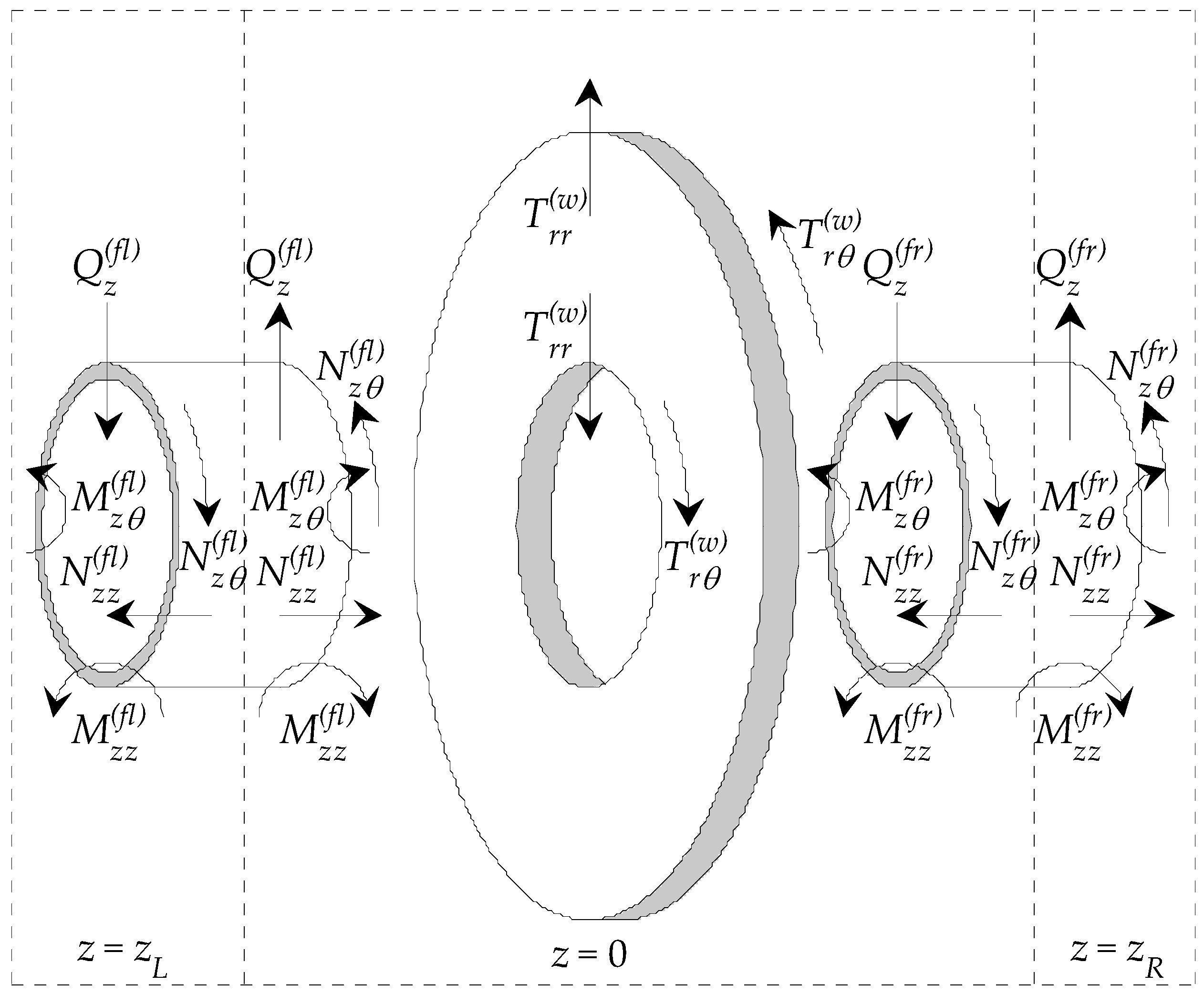
T r θ ( w ) ( r , θ ) = G v w ( r , θ ) r ( G r ) v w ( r , θ ) + ( G r ) w w ( r , θ ) θ   ,
T r θ ( w ) ( r , θ ) = n = 1 n = C 1 ( n ) { 2 G n k p r J n + 1 ( k p r ) 2 G n ( n 1 ) r 2 J n ( k p r ) } + C 2 ( n ) { 2 G n k p r Y n + 1 ( k p r ) 2 G n ( n 1 ) r 2 Y n ( k p r ) } + C 3 ( n ) { 2 G k s r J n + 1 ( k s r ) + G [ k s 2 r 2 2 ( n 2 n ) ] r 2 J n ( k s r ) } + C 4 ( n ) { 2 G k s r Y n + 1 ( k s r ) + G [ k s 2 r 2 2 ( n 2 n ) ] r 2 Y n ( k s r ) } sin ( n θ )
The solutions to the constants C1(n)C24(n) are found using equilibrium and continuity expressions from the system. Figure 4 is a free body diagram that shows the 24 individual generalized forces that are present on the boundaries of the system. The boundary conditions at the outer edge of the web (r = b) are
T r r ( w ) ( b , θ ) = n = 1 n = P n cos ( n θ )
and
T r θ ( w ) ( b , θ ) = n = 1 n = F n sin ( n θ )
where Pn is the magnitude of the radial external pressure and Fn is the magnitude of the circumferential external pressure for the n-indexed, non-axisymmetric load applied to the outer edge of the web. The five boundary conditions at the free edge of the left flange (z = zL) are
N z z ( f l ) ( θ , z L ) = M z z ( f l ) ( θ , z L ) = N z θ ( f l ) ( θ , z L ) = M z θ ( f l ) ( θ , z L ) = Q z ( f l ) ( θ , z L ) = 0   .
Similarly, the five boundary conditions at the free edge of the right flange (z = zR) are
N z z ( f r ) ( θ , z R ) = M z z ( f r ) ( θ , z R ) = N z θ ( f r ) ( θ , z R ) = M z θ ( f r ) ( θ , z R ) = Q z ( f r ) ( θ , z R ) = 0   .
There are three force balances at the intersection of the web and flange (r = a and z = 0). The force balance in the radial direction is
b w T r r ( w ) ( a , θ ) Q z ( f l ) ( θ , 0 ) + Q z ( f r ) ( θ , 0 ) = 0   ,
the force balance in the circumferential direction is
b w T r θ ( w ) ( a , θ ) N z θ ( f l ) ( θ , 0 ) + N z θ ( f r ) ( θ , 0 ) = 0
and the force balance in the longitudinal direction is
N z z ( f l ) ( θ , 0 ) + N z z ( f r ) ( θ , 0 ) = 0   .
Additionally, there are two moment balances at this location. The first is the bending moment in the longitudinal direction with respect to the longitudinal direction written as
M z z ( f l ) ( θ , 0 ) + M z z ( f r ) ( θ , 0 ) = 0
and the second is the twisting moment in the longitudinal direction with respect to the circumferential direction written as
M z θ ( f l ) ( θ , 0 ) + M z θ ( f r ) ( θ , 0 ) = 0   .
There are five displacement continuity equations at the intersection of the web and the flange, and these are written as
u f l ( θ , 0 ) = u f r ( θ , 0 )   ,
v w ( a , θ ) = v f l ( θ , 0 )   ,
v w ( a , θ ) = v f r ( θ , 0 )   ,
w w ( a , θ ) = w f l ( θ , 0 )
and
w w ( a , θ ) = w f r ( θ , 0 )   ,
and two slope continuity equations written as
ψ f l , z ( θ , 0 ) = ψ f r , z ( θ , 0 )
and
ψ f l , θ ( θ , 0 ) = ψ f r , θ ( θ , 0 )   .
Equations (53), (54) and (59) to (68) are equilibrium and continuity equations, they are orthogonalized in the circumferential direction, and this results in a decoupled n-indexed algebraic matrix equation given by
A n x n = b n   ,
where the entries of An are in Appendix D as Equations (A147) to (A478), the vector xn is
x n = { C 1 ( n ) C 2 ( n ) C 23 ( n ) C 24 ( n ) } T   ,
and the vector bn is
b n = { P n F n 0 0 } T   .
The solution to the wave propagation coefficients Ci(n)’s in Equation (123) is found using
x n = A n 1 b n   ,
and once these are known, they can be inserted back into Equations (53) and (54) to calculate the displacement of the web, Equations (59), (61), and (63) to calculate the displacements of the left flange or Equations (64), (66), and (68) to calculate the displacements of the right flange. The four dynamic stiffness components of the beam calculated from the model are
K r r ( n ) = b w P n W n ( b )   ,
K r θ ( n ) = K θ r ( n ) = b w F n W n ( b ) = b w P n V n ( b )
and
K θ θ ( n ) = b w F n V n ( b )   .
The longitudinal stiffness term K z z ( n ) is not calculated in this model. The previous curved beam model [1,2] utilized the Love–Kirchhoff plate equation for the out of plane motion of the web and the stiffness term K z z ( n ) could be calculated. For the geometry modeled here, this previous equation is accurate to about 5 kHz and then becomes too stiff. It is possible to include a higher-order plate model [24,25] to make this stiffness term more accurate. This plate model, however, includes terms that are extremely unstable when evaluated numerically, and even using extended precision analysis with a 256-bit word length only allowed numerical convergence up to about 6 kHz. Furthermore, most shell designs are very stiff in the longitudinal direction and an additional stiffness term in this direction does not affect the dynamic response. Thus, this term is not calculated and is set equal to zero in the reinforced shell model.

3. Results

The model was analyzed using an example problem where the beam had material and geometric properties that were consistent with an application to underwater structures. The model of the curved T beam had the following physical dimensions: height of the web hw = 0.244 m (9.60 in), width of the web bw = 0.0140 m (0.550 in), height of the flange h = hf = 0.0333 m (1.30 in), and width of the flange bf = 0.198 m (7.80 in), which results in the left flange free end at zL = − bf /2 = −0.0991 m and the right flange free end at zR = bf/2 = 0.0991 m. The outer radius of the beam is b = 3.00 m and the intersection of the flange and beam is at a = 2.76 m. The beam was made of steel, which had the following mechanical properties: Young’s modulus E = 200 × 109 N m−2, shear modulus G = 76.9 × 10⁹ N m−2, Poisson’s ratio υ = 0.30 and density ρ = 7800 kg m−3. The value for the shear correction factor was κ = 0.8333. Although any location of the beam can be chosen for displacement output, the web’s outer surface was investigated here because this location is pertinent to the analysis of reinforced cylindrical shells. This allowed the dynamic stiffness of the beam to be calculated and subsequently used in analysis of beams attached to shells or curved elastic bodies. To ensure the analytical model is accurate, the displacements were compared to results from a finite element model. The finite element displacements were produced using the COMSOL finite element program and the model consisted of 3400 quadratic serendipity axisymmetric solid elements which resulted in 32,523 degrees of freedom.
For the axisymmetric model, the beam was loaded on its outer surface with a radial (normal) pressure, commonly called a ring load. The output of this model is radial displacement divided by normal pressure at the web’s outer surface. Figure 5 is a comparison of normal displacement divided by normal pressure versus frequency for the n = 0 mode in the decibel scale referenced to m/Pa (or m/(N/m2)). The top plot is the analytical model compared to a fully elastic finite element solution, the middle plot is the analytical model compared to the previous analytical model [1,2] and the bottom plot is the analytical model compared to Bernoulli–Euler curved beam theory [22]. For this particular beam geometry, there was broad based agreement between the analytical model derived here and the finite element results up to approximately 47 kHz, while the previous analytical model is valid to about 8 kHz and the Bernoulli-Euler theory is valid to about 1.5 kHz.
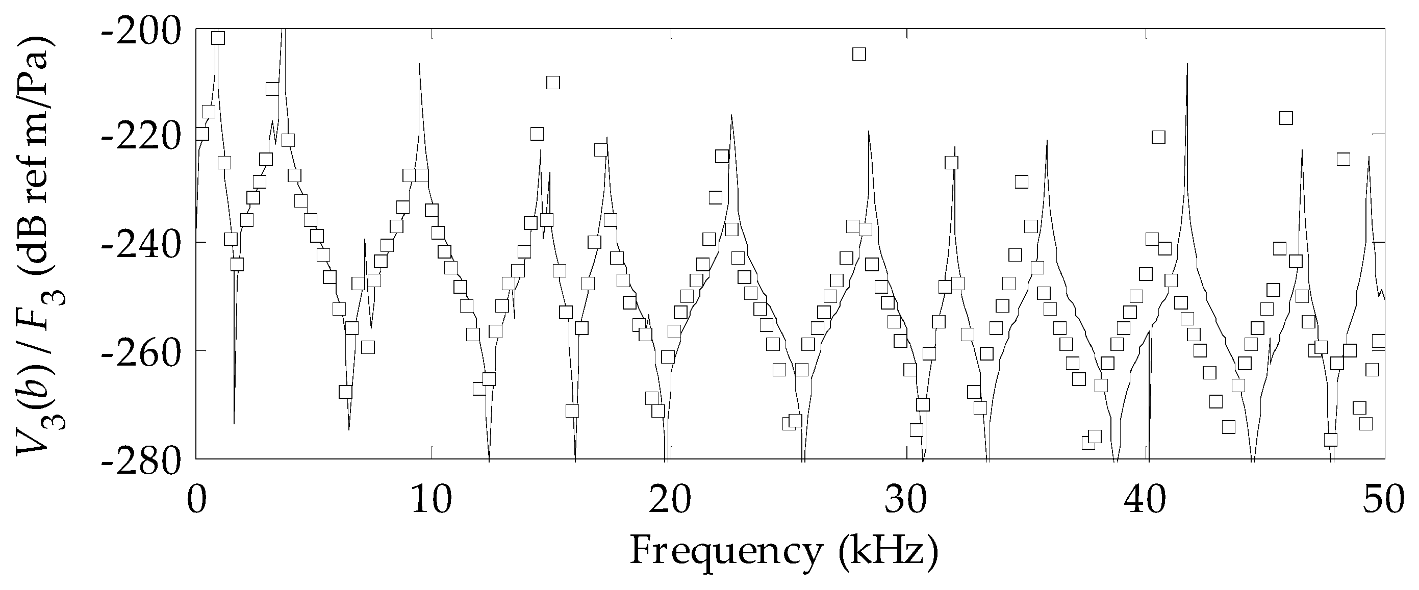
Higher order circumferential mode shapes (n > 0) were also investigated. For the non-axisymmetric model, the beam was loaded on its outer surface with a radial (normal) pressure and a tangential pressure, both corresponding to the circumferential mode number under investigation. The output of this model is radial displacement divided by normal pressure, radial displacement divided by tangential pressure (equal to tangential displacement divided by radial pressure) and tangential displacement divided by tangential pressure at the web’s outer surface. Figure 6 is a comparison of normal displacement divided by normal pressure versus frequency for the n = 3 mode, Figure 7 is a comparison of tangential displacement divided by tangential pressure versus frequency for the n = 3 mode, and Figure 8 is a comparison of tangential displacement divided by radial pressure versus frequency for the n = 3 mode. The dropout of the analytical model in Figure 7 around 40 kHz is most likely a frequency bin where the tangential displacement did not converge. This was the only location where this behavior was observed. The normal displacement divided by normal pressure was in agreement with the finite element results to about 47 kHz, the tangential displacement divided by radial pressure was in agreement with the finite element results to about 34 kHz, and the tangential displacement divided by tangential pressure was in agreement with the finite element results to about 47 kHz. Other values of n compared similarly. It is noted that by far the most important output of the model is normal displacement divided by normal pressure because this corresponds to the most compliant direction of a shell reinforced with a circular beam. The run time of the COMSOL finite element model was 1320 s versus 0.22 s for the analytical model, which makes the analytical model about four orders of magnitude faster than this finite element model.

4. Conclusions

A high frequency analytical model for a circular T-shaped beam was derived and compared to results obtained from a fully elastic finite element model, a previous analytical model and Bernoulli-Euler curved beam theory. This new model was constructed with two-dimensional elastic equations for the web motion and Timoshenko shell equations for the flange motion. Adding the Timoshenko shell equations to this model resulted in additional degrees of freedom which produced much more accurate results at higher frequencies. The outputs of this new model are normal displacement divided by normal pressure, normal displacement divided by tangential pressure, tangential displacement divided by normal pressure and tangential displacement divided by tangential pressure. It is noted that by far the most important output is normal displacement divided by normal pressure, as this corresponds to the design objective of almost all beams. The resultant normal and tangential circular beam stiffness terms were also derived. The longitudinal stiffness term of the beam was briefly discussed. This new model allows for an almost total elastic response of the entire system for the frequency ranges studied, and for the beam example problem presented here, the analytical model and the finite element models compared favorably up to 47 kHz for normal displacement divided by normal pressure. The valid frequency ranges of the Bernoulli–Euler and pervious analytical model are depicted in a comparison of mode n = 0 response and were 1.5 kHz and 8 kHz respectively. The application of this model to a reinforced structure for target strength and hull response modeling is discussed. This new analytical model was approximately four orders of magnitude faster than the finite element model for the example problem presented in this paper, and thus can be used in the design phase of structures where rapid analysis is needed. Typically, finite element analysis is too slow for analyzing numerous designs.

Author Contributions

Conceptualization, A.J.H. and D.P.; analytical software, A.J.H.; finite element software, D.P.; validation, A.J.H. and D.P.; writing—original draft preparation, A.J.H.; writing—review and editing, A.J.H. and D.P.; and funding acquisition, A.J.H.

Funding

This work was funded by the Office of Naval Research (ONR) Naval Undersea Research Program (NURP).

Acknowledgments

The authors wish to thank Maria Medeiros of ONR Sea Platforms and Weapons Division.

Conflicts of Interest

The authors declare no conflicts of interest. Additionally, “the funding sponsors had no role in the design of the study; in the collection, analyses, or interpretation of data; in the writing of the manuscript, and in the decision to publish the results”.

Appendix A

The constants from Equation (28) are listed in this appendix.
a 6 = ( 1 a 2 ) D κ G h ( E p a 2 + D )   ,
a 4 =   ( D 3 a 6 ) ( 1 a 2 ) [ D ( E p 2 E p 2 υ 2 + D h ω 2 ρ 2 E p κ G h υ + 2 κ G I h ω 2 ρ ) ] + h ω 2 ρ ( D E p + E p κ G I + D κ G h )   ,
a 2 =   ( D a 4 ) ( E p I ω 2 ρ D h ω 2 ρ + E p κ G h ) ( 1 a 2 ) ( E p 2 I υ 2 ω 2 ρ + E p 2 I ω 2 ρ + κ G h E p 2 υ 2 κ G h E p 2 2 κ G h E p I υ ω 2 ρ + D h E p ω 2 ρ + κ G h I 2 ω 4 ρ 2 + 2 D h I ω 4 ρ 2 ) + h ω 2 ρ ( E p I ω 2 ρ + D h ω 2 ρ κ G h E p + κ G h I ω 2 ρ ) + ( 1 a 6 ) 2 D 2 I ω 2 ρ
and
a 0 = ( 1 a 6 ) ω 2 ρ ( ω 2 ρ I 2 ω 2 ρ I a 2 h + κ G a 2 h 2 ) ( ω 2 ρ h a 4 + E p a 2 + D )   .

Appendix B

The non-zero entries to the A0 matrix in Equation (48) are listed in this appendix.
a 1 , 1 = E k p b ( 1 + υ ) J 1 ( k p b ) E k p 2 ( 1 υ 2 ) J 0 ( k p b )   ,
a 1 , 2 = E k p b ( 1 + υ ) Y 1 ( k p b ) E k p 2 ( 1 υ 2 ) Y 0 ( k p b )   ,
a 2 , 1 = b w E k p a ( 1 + υ ) J 1 ( k p a ) b w E k p 2 ( 1 υ 2 ) J 0 ( k p a )   ,
a 2 , 2 = b w E k p a ( 1 + υ ) Y 1 ( k p a ) b w E k p 2 ( 1 υ 2 ) Y 0 ( k p a )   ,
a 2 , 3 = κ G h   ( λ 1 ( 0 ) + N 1 ( 0 ) )   ,
a 2 , 4 = κ G h   ( λ 2 ( 0 ) + N 2 ( 0 ) )   ,
a 2 , 5 = κ G h   ( λ 3 ( 0 ) + N 3 ( 0 ) )   ,
a 2 , 6 = κ G h   ( λ 4 ( 0 ) + N 4 ( 0 ) )   ,
a 2 , 7 = κ G h   ( λ 5 ( 0 ) + N 5 ( 0 ) )   ,
a 2 , 8 = κ G h   ( λ 6 ( 0 ) + N 6 ( 0 ) )   ,
a 2 , 9 = κ G h   ( λ 1 ( 0 ) + N 1 ( 0 ) )   ,
a 2 , 10 = κ G h   ( λ 2 ( 0 ) + N 2 ( 0 ) )   ,
a 2 , 11 = κ G h   ( λ 3 ( 0 ) + N 3 ( 0 ) )   ,
a 2 , 12 = κ G h   ( λ 4 ( 0 ) + N 4 ( 0 ) )   ,
a 2 , 13 = κ G h   ( λ 5 ( 0 ) + N 5 ( 0 ) )   ,
a 2 , 14 = κ G h   ( λ 6 ( 0 ) + N 6 ( 0 ) )   ,
a 3 , 3 = υ E p a E p M 1 ( 0 ) λ 1 ( 0 ) D N 1 ( 0 ) λ 1 ( 0 ) a   ,
a 3 , 4 = υ E p a E p M 2 ( 0 ) λ 2 ( 0 ) D N 2 ( 0 ) λ 2 ( 0 ) a   ,
a 3 , 5 = υ E p a E p M 3 ( 0 ) λ 3 ( 0 ) D N 3 ( 0 ) λ 3 ( 0 ) a   , .  
a 3 , 6 = υ E p a E p M 4 ( 0 ) λ 4 ( 0 ) D N 4 ( 0 ) λ 4 ( 0 ) a   ,
a 3 , 7 = υ E p a E p M 5 ( 0 ) λ 5 ( 0 ) D N 5 ( 0 ) λ 5 ( 0 ) a   ,
a 3 , 8 = υ E p a E p M 6 ( 0 ) λ 6 ( 0 ) D N 6 ( 0 ) λ 6 ( 0 ) a   ,
a 3 , 9 = υ E p a + E p M 1 ( 0 ) λ 1 ( 0 ) + D N 1 ( 0 ) λ 1 ( 0 ) a   ,
a 3 , 10 = υ E p a + E p M 2 ( 0 ) λ 2 ( 0 ) + D N 2 ( 0 ) λ 2 ( 0 ) a   ,
a 3 , 11 = υ E p a + E p M 3 ( 0 ) λ 3 ( 0 ) + D N 3 ( 0 ) λ 3 ( 0 ) a   ,
a 3 , 12 = υ E p a + E p M 4 ( 0 ) λ 4 ( 0 ) + D N 4 ( 0 ) λ 4 ( 0 ) a   ,
a 3 , 13 = υ E p a + E p M 5 ( 0 ) λ 5 ( 0 ) + D N 5 ( 0 ) λ 5 ( 0 ) a   ,
a 3 , 14 = υ E p a + E p M 6 ( 0 ) λ 6 ( 0 ) + D N 6 ( 0 ) λ 6 ( 0 ) a   ,
a 4 , 3 = D M 1 ( 0 ) λ 1 ( 0 ) a D N 1 ( 0 ) λ 1 ( 0 )   ,
a 4 , 4 = D M 2 ( 0 ) λ 2 ( 0 ) a D N 2 ( 0 ) λ 2 ( 0 )   ,
a 4 , 5 = D M 3 ( 0 ) λ 3 ( 0 ) a D N 3 ( 0 ) λ 3 ( 0 )   ,
a 4 , 6 = D M 4 ( 0 ) λ 4 ( 0 ) a D N 4 ( 0 ) λ 4 ( 0 )   ,
a 4 , 7 = D M 5 ( 0 ) λ 5 ( 0 ) a D N 5 ( 0 ) λ 5 ( 0 )   ,
a 4 , 8 = D M 6 ( 0 ) λ 6 ( 0 ) a D N 6 ( 0 ) λ 6 ( 0 )   ,
a 4 , 9 = D M 1 ( 0 ) λ 1 ( 0 ) a + D N 1 ( 0 ) λ 1 ( 0 )   ,
a 4 , 10 = D M 2 ( 0 ) λ 2 ( 0 ) a + D N 2 ( 0 ) λ 2 ( 0 )   ,
a 4 , 11 = D M 3 ( 0 ) λ 3 ( 0 ) a + D N 3 ( 0 ) λ 3 ( 0 )   ,
a 4 , 12 = D M 4 ( 0 ) λ 4 ( 0 ) a + D N 4 ( 0 ) λ 4 ( 0 )   ,
a 4 , 13 = D M 5 ( 0 ) λ 5 ( 0 ) a + D N 5 ( 0 ) λ 5 ( 0 )   ,
a 4 , 14 = D M 6 ( 0 ) λ 6 ( 0 ) a + D N 6 ( 0 ) λ 6 ( 0 )   ,
a 5 , 3 = M 1 ( 0 )   ,
a 5 , 4 = M 2 ( 0 )   ,
a 5 , 5 = M 3 ( 0 )   ,
a 5 , 6 = M 4 ( 0 )   ,
a 5 , 7 = M 5 ( 0 )   ,
a 5 , 8 = M 6 ( 0 )   ,
a 5 , 9 = M 1 ( 0 )   ,
a 5 , 10 = M 2 ( 0 )   ,
a 5 , 11 = M 3 ( 0 )   ,
a 5 , 12 = M 4 ( 0 )   ,
a 5 , 13 = M 5 ( 0 )   ,
a 5 , 14 = M 6 ( 0 )   ,
a 6 , 1 = k p J 1 ( k p a )   ,
a 6 , 2 = k p Y 1 ( k p a )   ,
a 6 , 3 = 1   ,
a 6 , 4 = 1   ,
a 6 , 5 = 1   ,
a 6 , 6 = 1   ,
a 6 , 7 = 1   ,
a 6 , 8 = 1   ,
a 7 , 1 = k p J 1 ( k p a )   ,
a 7 , 2 = k p Y 1 ( k p a )   ,
a 7 , 9 = 1   ,
a 7 , 10 = 1   ,
a 7 , 11 = 1   ,
a 7 , 12 = 1   ,
a 7 , 13 = 1   ,
a 7 , 14 = 1   ,
a 8 , 3 = N 1 ( 0 )   ,
a 8 , 4 = N 2 ( 0 )   ,
a 8 , 5 = N 3 ( 0 )   ,
a 8 , 6 = N 4 ( 0 )   ,
a 8 , 7 = N 5 ( 0 )   ,
a 8 , 8 = N 6 ( 0 )   ,
a 8 , 9 = N 1 ( 0 )   ,
a 8 , 10 = N 2 ( 0 )   ,
a 8 , 11 = N 3 ( 0 )   ,
a 8 , 12 = N 4 ( 0 )   ,
a 8 , 13 = N 5 ( 0 )   ,
a 8 , 14 = N 6 ( 0 )   ,
a 9 , 3 = exp ( λ 1 ( 0 ) z L ) [ υ E p a + E p M 1 ( 0 ) λ 1 ( 0 ) + D N 1 ( 0 ) λ 1 ( 0 ) a ]   ,
a 9 , 4 = exp ( λ 2 ( 0 ) z L ) [ υ E p a + E p M 2 ( 0 ) λ 2 ( 0 ) + D N 2 ( 0 ) λ 2 ( 0 ) a ]   ,
a 9 , 5 = exp ( λ 3 ( 0 ) z L ) [ υ E p a + E p M 3 ( 0 ) λ 3 ( 0 ) + D N 3 ( 0 ) λ 3 ( 0 ) a ]   ,
a 9 , 6 = exp ( λ 4 ( 0 ) z L ) [ υ E p a + E p M 4 ( 0 ) λ 4 ( 0 ) + D N 4 ( 0 ) λ 4 ( 0 ) a ]   ,
a 9 , 7 = exp ( λ 5 ( 0 ) z L ) [ υ E p a + E p M 5 ( 0 ) λ 5 ( 0 ) + D N 5 ( 0 ) λ 5 ( 0 ) a ]   ,
a 9 , 8 = exp ( λ 6 ( 0 ) z L ) [ υ E p a + E p M 6 ( 0 ) λ 6 ( 0 ) + D N 6 ( 0 ) λ 6 ( 0 ) a ]   ,
a 10 , 3 = exp ( λ 1 ( 0 ) z L )   κ G h   ( λ 1 ( 0 ) + N 1 ( 0 ) )   ,
a 10 , 4 = exp ( λ 2 ( 0 ) z L )   κ G h   ( λ 2 ( 0 ) + N 2 ( 0 ) )   ,
a 10 , 5 = exp ( λ 3 ( 0 ) z L )   κ G h   ( λ 3 ( 0 ) + N 3 ( 0 ) )   ,
a 10 , 6 = exp ( λ 4 ( 0 ) z L )   κ G h   ( λ 4 ( 0 ) + N 4 ( 0 ) )   ,
a 10 , 7 = exp ( λ 5 ( 0 ) z L )   κ G h   ( λ 5 ( 0 ) + N 5 ( 0 ) )   ,
a 10 , 8 = exp ( λ 6 ( 0 ) z L )   κ G h   ( λ 6 ( 0 ) + N 6 ( 0 ) )   ,
a 11 , 3 = exp ( λ 1 ( 0 ) z L ) [ D M 1 ( 0 ) λ 1 ( 0 ) a + D N 1 ( 0 ) λ 1 ( 0 ) ]   ,
a 11 , 4 = exp ( λ 2 ( 0 ) z L ) [ D M 2 ( 0 ) λ 2 ( 0 ) a + D N 2 ( 0 ) λ 2 ( 0 ) ]   ,
a 11 , 5 = exp ( λ 3 ( 0 ) z L ) [ D M 3 ( 0 ) λ 3 ( 0 ) a + D N 3 ( 0 ) λ 3 ( 0 ) ]   ,
a 11 , 6 = exp ( λ 4 ( 0 ) z L ) [ D M 4 ( 0 ) λ 4 ( 0 ) a + D N 4 ( 0 ) λ 4 ( 0 ) ]   ,
a 11 , 7 = exp ( λ 5 ( 0 ) z L ) [ D M 5 ( 0 ) λ 5 ( 0 ) a + D N 5 ( 0 ) λ 5 ( 0 ) ]   ,
a 11 , 8 = exp ( λ 6 ( 0 ) z L ) [ D M 6 ( 0 ) λ 6 ( 0 ) a + D N 6 ( 0 ) λ 6 ( 0 ) ]   ,
a 12 , 9 = exp ( λ 1 ( 0 ) z R ) [ υ E p a + E p M 1 ( 0 ) λ 1 ( 0 ) + D N 1 ( 0 ) λ 1 ( 0 ) a ]   ,
a 12 , 10 = exp ( λ 2 ( 0 ) z R ) [ υ E p a + E p M 2 ( 0 ) λ 2 ( 0 ) + D N 2 ( 0 ) λ 2 ( 0 ) a ]   ,
a 12 , 11 = exp ( λ 3 ( 0 ) z R ) [ υ E p a + E p M 3 ( 0 ) λ 3 ( 0 ) + D N 3 ( 0 ) λ 3 ( 0 ) a ]   ,
a 12 , 12 = exp ( λ 4 ( 0 ) z R ) [ υ E p a + E p M 4 ( 0 ) λ 4 ( 0 ) + D N 4 ( 0 ) λ 4 ( 0 ) a ]   ,
a 12 , 13 = exp ( λ 5 ( 0 ) z R ) [ υ E p a + E p M 5 ( 0 ) λ 5 ( 0 ) + D N 5 ( 0 ) λ 5 ( 0 ) a ]   ,
a 12 , 14 = exp ( λ 6 ( 0 ) z R ) [ υ E p a + E p M 6 ( 0 ) λ 6 ( 0 ) + D N 6 ( 0 ) λ 6 ( 0 ) a ]   ,
a 13 , 9 = exp ( λ 1 ( 0 ) z R )   κ G h   ( λ 1 ( 0 ) + N 1 ( 0 ) )   ,
a 13 , 10 = exp ( λ 2 ( 0 ) z R )   κ G h   ( λ 2 ( 0 ) + N 2 ( 0 ) )   ,
a 13 , 11 = exp ( λ 3 ( 0 ) z R )   κ G h   ( λ 3 ( 0 ) + N 3 ( 0 ) )   ,
a 13 , 12 = exp ( λ 4 ( 0 ) z R )   κ G h   ( λ 4 ( 0 ) + N 4 ( 0 ) )   ,
a 13 , 13 = exp ( λ 5 ( 0 ) z R )   κ G h   ( λ 5 ( 0 ) + N 5 ( 0 ) )   ,
a 13 , 14 = exp ( λ 6 ( 0 ) z R )   κ G h   ( λ 6 ( 0 ) + N 6 ( 0 ) )   ,
a 14 , 9 = exp ( λ 1 ( 0 ) z R ) [ D M 1 ( 0 ) λ 1 ( 0 ) a + D N 1 ( 0 ) λ 1 ( 0 ) ]   ,
a 14 , 10 = exp ( λ 2 ( 0 ) z R ) [ D M 2 ( 0 ) λ 2 ( 0 ) a + D N 2 ( 0 ) λ 2 ( 0 ) ]   ,
a 14 , 11 = exp ( λ 3 ( 0 ) z R ) [ D M 3 ( 0 ) λ 3 ( 0 ) a + D N 3 ( 0 ) λ 3 ( 0 ) ]   ,
a 14 , 12 = exp ( λ 4 ( 0 ) z R ) [ D M 4 ( 0 ) λ 4 ( 0 ) a + D N 4 ( 0 ) λ 4 ( 0 ) ]   ,
a 14 , 13 = exp ( λ 5 ( 0 ) z R ) [ D M 5 ( 0 ) λ 5 ( 0 ) a + D N 5 ( 0 ) λ 5 ( 0 ) ]
and
a 14 , 14 = exp ( λ 6 ( 0 ) z R ) [ D M 6 ( 0 ) λ 6 ( 0 ) a + D N 6 ( 0 ) λ 6 ( 0 ) ]   .

Appendix C

The constants from Equation (91) are listed in this appendix.
a 10 = b 29 ( b 03 2 + b 01 b 09 ) ( b 16 2 + b 14 b 22 )   ,
a 8 = ( b 12 2 b 14 b 22 b 12 2 b 16 2 + b 11 2 b 14 b 29 b 09 b 16 2 b 30 b 10 b 16 2 b 29 2 b 09 b 16 b 17 b 29 + b 09 b 14 b 22 b 30 + b 09 b 14 b 23 b 29 + b 09 b 15 b 22 b 29 + b 10 b 14 b 22 b 29 ) b 01 + b 03 2 b 16 2 b 30 b 06 2 b 09 b 16 2 + 2 b 03 b 06 b 12 b 16 2 + b 06 2 b 09 b 14 b 22 + 2 b 03 b 04 b 16 2 b 29 b 02 b 09 b 16 2 b 29 + 2 b 03 2 b 16 b 17 b 29 + b 05 2 b 09 b 22 b 29 b 03 2 b 14 b 22 b 30 b 03 2 b 14 b 23 b 29 b 03 2 b 15 b 22 b 29 2 b 03 b 06 b 12 b 14 b 22 + 2 b 03 b 05 b 11 b 16 b 29 2 b 03 b 04 b 14 b 22 b 29 + b 02 b 09 b 14 b 22 b 29   ,
a 6 = ( b 12 2 b 14 b 23 b 09 b 14 b 24 2 b 09 b 18 2 b 22 2 b 12 2 b 16 b 17 + b 12 2 b 15 b 22 b 09 b 17 2 b 29 + b 11 2 b 14 b 30 + b 11 2 b 15 b 29 b 10 b 16 2 b 30 + 2 b 11 b 12 b 16 b 18 2 b 11 b 12 b 14 b 24 + 2 b 09 b 16 b 18 b 24 2 b 09 b 16 b 17 b 30 2 b 10 b 16 b 17 b 29 + b 09 b 14 b 23 b 30 + b 09 b 15 b 22 b 30 + b 09 b 15 b 23 b 29 +   b 10 b 14 b 22 b 30 + b 10 b 14 b 23 b 29 + b 10 b 15 b 22 b 29 ) b 01 + b 06 2 b 11 2 b 14 b 02 b 12 2 b 16 2 b 06 2 b 10 b 16 2 + b 05 2 b 12 2 b 22 + b 03 2 b 14 b 24 2 + b 03 2 b 18 2 b 22 + b 05 2 b 11 2 b 29 + b 03 2 b 17 2 b 29 + b 04 2 b 16 2 b 29 + 2 b 04 b 06 b 12 b 16 2 2 b 06 2 b 09 b 16 b 17 + b 02 b 12 2 b 14 b 22 + b 06 2 b 09 b 14 b 23 + b 06 2 b 09 b 15 b 22 + b 06 2 b 10 b 14 b 22 + 2 b 03 b 04 b 16 2 b 30 + b 02 b 11 2 b 14 b 29 b 02 b 09 b 16 2 b 30 b 02 b 10 b 16 2 b 29 2 b 03 2 b 16 b 18 b 24 + 2 b 03 2 b 16 b 17 b 30 + b 05 2 b 09 b 22 b 30 + b 05 2 b 09 b 23 b 29 + b 05 2 b 10 b 22 b 29 b 04 2 b 14 b 22 b 29 b 03 2 b 14 b 23 b 30 b 03 2 b 15 b 22 b 30 b 03 2 b 15 b 23 b 29 +   2 b 05 b 06 b 11 b 12 b 16 2 b 03 b 06 b 11 b 16 b 18 + 4 b 03 b 06 b 12 b 16 b 17 + 2 b 03 b 06 b 11 b 14 b 24 2 b 03 b 06 b 12 b 14 b 23 2 b 03 b 06 b 12 b 15 b 22 2 b 04 b 06 b 12 b 14 b 22 2 b 03 b 05 b 12 b 16 b 24 + 2 b 03 b 05 b 12 b 18 b 22 + 2 b 05 b 06 b 09 b 16 b 24 2 b 05 b 06 b 09 b 18 b 22 + 2 b 03 b 05 b 11 b 16 b 30 + 2 b 03 b 05 b 11 b 17 b 29 + 2 b 04 b 05 b 11 b 16 b 29 + 4 b 03 b 04 b 16 b 17 b 29 2 b 02 b 09 b 16 b 17 b 29 2 b 03 b 04 b 14 b 22 b 30 2 b 03 b 04 b 14 b 23 b 29 2 b 03 b 04 b 15 b 22 b 29 + b 02 b 09 b 14 b 22 b 30 + b 02 b 09 b 14 b 23 b 29 + b 02 b 09 b 15 b 22 b 29 + b 02 b 10 b 14 b 22 b 29   ,
a 4 = ( b 12 2 b 15 b 23   b 12 2 b 17 2 b 09 b 15 b 24 2 b 10 b 14 b 24 2 b 09 b 18 2 b 23 b 10 b 18 2 b 22 b 11 2 b 18 2 b 09 b 17 2 b 30 b 10 b 17 2 b 29 + b 11 2 b 15 b 30 + 2 b 11 b 12 b 17 b 18 2 b 11 b 12 b 15 b 24 + 2 b 09 b 17 b 18 b 24 + 2 b 10 b 16 b 18 b 24 2 b 10 b 16 b 17 b 30 + b 09 b 15 b 23 b 30 + b 10 b 14 b 23 b 30 + b 10 b 15 b 22 b 30 +   b 10 b 15 b 23 b 29 ) b 01 + b 06 2 b 11 2 b 15 b 06 2 b 09 b 17 2 b 05 2 b 09 b 24 2 + b 05 2 b 12 2 b 23 +   b 03 2 b 15 b 24 2 + b 03 2 b 18 2 b 23 + b 05 2 b 11 2 b 30 + b 03 2 b 17 2 b 30 + b 04 2 b 16 2 b 30 + 2 b 03 b 06 b 12 b 17 2 2 b 05 b 06 b 11 2 b 18 + 2 b 03 b 04 b 14 b 24 2 2 b 02 b 12 2 b 16 b 17 + 2 b 03 b 04 b 18 2 b 22 b 02 b 09 b 14 b 24 2 2 b 06 2 b 10 b 16 b 17 b 02 b 09 b 18 2 b 22 + b 02 b 12 2 b 14 b 23 + b 02 b 12 2 b 15 b 22 2 b 05 2 b 11 b 12 b 24 + 2 b 03 b 04 b 17 2 b 29 + b 06 2 b 09 b 15 b 23 + b 06 2 b 10 b 14 b 23 + b 06 2 b 10 b 15 b 22 b 02 b 09 b 17 2 b 29 + b 02 b 11 2 b 14 b 30 + b 02 b 11 2 b 15 b 29 b 02 b 10 b 16 2 b 30 2 b 03 2 b 17 b 18 b 24 + 2 b 04 2 b 16 b 17 b 29 + b 05 2 b 09 b 23 b 30 +   b 05 2 b 10 b 22 b 30 + b 05 2 b 10 b 23 b 29 b 04 2 b 14 b 22 b 30 b 04 2 b 14 b 23 b 29 b 04 2 b 15 b 22 b 29 b 03 2 b 15 b 23 b 30 + 2 b 05 b 06 b 11 b 12 b 17 2 b 03 b 06 b 11 b 17 b 18 2 b 04 b 06 b 11 b 16 b 18 + 4 b 04 b 06 b 12 b 16 b 17 + 2 b 02 b 11 b 12 b 16 b 18 + 2 b 03 b 06 b 11 b 15 b 24 2 b 03 b 06 b 12 b 15 b 23 + 2 b 04 b 06 b 11 b 14 b 24 2 b 04 b 06 b 12 b 14 b 23 2 b 04 b 06 b 12 b 15 b 22 2 b 03 b 05 b 11 b 18 b 24 2 b 03 b 05 b 12 b 17 b 24 + 2 b 03 b 05 b 12 b 18 b 23 2 b 04 b 05 b 12 b 16 b 24 + 2 b 04 b 05 b 12 b 18 b 22 + 2 b 05 b 06 b 09 b 17 b 24 2 b 05 b 06 b 09 b 18 b 23 + 2 b 05 b 06 b 10 b 16 b 24 2 b 05 b 06 b 10 b 18 b 22 2 b 02 b 11 b 12 b 14 b 24 4 b 03 b 04 b 16 b 18 b 24 + 2 b 03 b 05 b 11 b 17 b 30 + 2 b 04 b 05 b 11 b 16 b 30 + 2 b 04 b 05 b 11 b 17 b 29 + 2 b 02 b 09 b 16 b 18 b 24 + 4 b 03 b 04 b 16 b 17 b 30 2 b 02 b 09 b 16 b 17 b 30 2 b 02 b 10 b 16 b 17 b 29 2 b 03 b 04 b 14 b 23 b 30 2 b 03 b 04 b 15 b 22 b 30 2 b 03 b 04 b 15 b 23 b 29 + b 02 b 09 b 14 b 23 b 30 + b 02 b 09 b 15 b 22 b 30 + b 02 b 09 b 15 b 23 b 29 + b 02 b 10 b 14 b 22 b 30 + b 02 b 10 b 14 b 23 b 29 + b 02 b 10 b 15 b 22 b 29   ,
a 2 = ( b 10 b 30 b 17 2 + 2 b 10 b 17 b 18 b 24 b 10 b 23 b 18 2 b 10 b 15 b 24 2 + b 10 b 15 b 23 b 30 ) b 01 + b 04 2 b 14 b 24 2 b 02 b 12 2 b 17 2 b 06 2 b 10 b 17 2 b 05 2 b 10 b 24 2 b 02 b 11 2 b 18 2 + b 04 2 b 18 2 b 22 + b 04 2 b 17 2 b 29 + 2 b 04 b 06 b 12 b 17 2 + 2 b 03 b 04 b 15 b 24 2 + 2 b 03 b 04 b 18 2 b 23 b 02 b 09 b 15 b 24 2 b 02 b 10 b 14 b 24 2 b 02 b 09 b 18 2 b 23 b 02 b 10 b 18 2 b 22 + b 02 b 12 2 b 15 b 23 + 2 b 03 b 04 b 17 2 b 30 + b 06 2 b 10 b 15 b 23 b 02 b 09 b 17 2 b 30 b 02 b 10 b 17 2 b 29 + b 02 b 11 2 b 15 b 30 2 b 04 2 b 16 b 18 b 24 + 2 b 04 2 b 16 b 17 b 30 + b 05 2 b 10 b 23 b 30 b 04 2 b 14 b 23 b 30 b 04 2 b 15 b 22 b 30 b 04 2 b 15 b 23 b 29 2 b 04 b 06 b 11 b 17 b 18 + 2 b 02 b 11 b 12 b 17 b 18 + 2 b 04 b 06 b 11 b 15 b 24 2 b 04 b 06 b 12 b 15 b 23 2 b 04 b 05 b 11 b 18 b 24 2 b 04 b 05 b 12 b 17 b 24 + 2 b 04 b 05 b 12 b 18 b 23 + 2 b 05 b 06 b 10 b 17 b 24 2 b 05 b 06 b 10 b 18 b 23 2 b 02 b 11 b 12 b 15 b 24 4 b 03 b 04 b 17 b 18 b 24 + 2 b 04 b 05 b 11 b 17 b 30 + 2 b 02 b 09 b 17 b 18 b 24 + 2 b 02 b 10 b 16 b 18 b 24 2 b 02 b 10 b 16 b 17 b 30 2 b 03 b 04 b 15 b 23 b 30 + b 02 b 09 b 15 b 23 b 30 + b 02 b 10 b 14 b 23 b 30 + b 02 b 10 b 15 b 22 b 30 + b 02 b 10 b 15 b 23 b 29
and
a 0 = ( b 04 2 + b 02 b 10 ) ( b 30 b 17 2 2 b 17 b 18 b 24 + b 23 b 18 2 + b 15 b 24 2 b 15 b 23 b 30 )   ,
where
b 01 = E p   ,
b 02 = h ω 2 ρ ( 1 a 2 ) [ G h n 2 ( I a 2 h + 1 ) ]   ,
b 03 = D a   ,
b 04 = G I n 2 a 3 + I ω 2 ρ a   ,
b 05 = E p n ( 1 + υ ) 2 a   ,
b 06 = E p υ a   ,
b 09 = D   ,
b 10 = κ G h + I ω 2 ρ G I n 2 a 2   ,
b 11 = D n ( 1 + υ ) 2 a   ,
b 12 = κ G h   ,
b 14 = G h   ,
b 15 = n 2 ( D a 4 + E p a 2 ) + h ω 2 ρ κ G a 2 ( h + I a 2 )   ,
b 16 = G I a   ,
b 17 = D n 2 a 3 + I ω 2 ρ a κ G a ( h + I a 2 )   ,
b 18 = n [ D a 4 + E p a 2 + κ G a 2 ( h + I a 2 ) ]   ,
b 22 = G I   ,
b 23 = I ω 2 ρ D n 2 a 2 κ G ( h + I a 2 )   ,
b 24 = n [ D a 3 + κ G a ( h + I a 2 ) ]   ,
b 29 = κ G h
and
b 30 = h ω 2 ρ ( D a 4 + E p a 2 ) κ G n 2 a 2 ( h + I a 2 )   .

Appendix D

The non-zero entries to the An matrix in Equation (123) are listed in this appendix.
a 1 , 1 = E k p b ( 1 + υ ) J n + 1 ( k p b ) E ( n n 2 ) ( 1 υ ) + k p 2 b 2 b 2 ( 1 υ 2 ) J n ( k p b )   ,
a 1 , 2 = E k p b ( 1 + υ ) Y n + 1 ( k p b ) E ( n n 2 ) ( 1 υ ) + k p 2 b 2 b 2 ( 1 υ 2 ) Y n ( k p b )   ,
a 1 , 3 = E n k s b ( 1 + υ ) J n + 1 ( k s b ) + E n ( n 1 ) b 2 ( 1 + υ ) J n ( k s b )   ,
a 1 , 4 = E n k s b ( 1 + υ ) Y n + 1 ( k s b ) + E n ( n 1 ) b 2 ( 1 + υ ) Y n ( k s b )   ,
a 2 , 1 = 2 G n k p b J n + 1 ( k p b ) + 2 G n ( n 1 ) b 2 J n ( k p b )   ,
a 2 , 2 = 2 G n k p b Y n + 1 ( k p b ) + 2 G n ( n 1 ) b 2 Y n ( k p b )   ,
a 2 , 3 = 2 G k s b J n + 1 ( k s b ) + G [ k s 2 b 2 2 ( n 2 n ) ] b 2 J n ( k s b )   ,
a 2 , 4 = 2 G k s b Y n + 1 ( k s b ) + G [ k s 2 b 2 2 ( n 2 n ) ] b 2 Y n ( k s b )   ,
a 3 , 1 = b w E k p a ( 1 + υ ) J n + 1 ( k p a ) b w [ E ( n n 2 ) ( 1 υ ) k p 2 a 2 ] a 2 ( 1 υ 2 ) J n ( k p a )   ,
a 3 , 2 = b w E k p a ( 1 + υ ) Y n + 1 ( k p a ) b w [ E ( n n 2 ) ( 1 υ ) k p 2 a 2 ] a 2 ( 1 υ 2 ) Y n ( k p a )   ,
a 3 , 3 = b w E n k s a ( 1 + υ ) J n + 1 ( k s a ) + b w E n ( n 1 ) a 2 ( 1 + υ ) J n ( k s a )   ,
a 3 , 4 = b w E n k s a ( 1 + υ ) Y n + 1 ( k s a ) + b w E n ( n 1 ) a 2 ( 1 + υ ) Y n ( k s a )   ,
a 3 , 5 = κ G h   ( λ 1 ( n ) + N 1 ( n ) )   ,
a 3 , 6 = κ G h   ( λ 2 ( n ) + N 2 ( n ) )   ,
a 3 , 7 = κ G h   ( λ 3 ( n ) + N 3 ( n ) )   ,
a 3 , 8 = κ G h   ( λ 4 ( n ) + N 4 ( n ) )   ,
a 3 , 9 = κ G h   ( λ 5 ( n ) + N 5 ( n ) )   ,
a 3 , 10 = κ G h   ( λ 6 ( n ) + N 6 ( n ) )   ,
a 3 , 11 = κ G h   ( λ 7 ( n ) + N 7 ( n ) )   ,
a 3 , 12 = κ G h   ( λ 8 ( n ) + N 8 ( n ) )   ,
a 3 , 13 = κ G h   ( λ 9 ( n ) + N 9 ( n ) )   ,
a 3 , 14 = κ G h   ( λ 10 ( n ) + N 10 ( n ) )   ,
a 3 , 15 = κ G h   ( λ 1 ( n ) + N 1 ( n ) )   ,
a 3 , 16 = κ G h   ( λ 2 ( n ) + N 2 ( n ) )   ,
a 3 , 17 = κ G h   ( λ 3 ( n ) + N 3 ( n ) )   ,
a 3 , 18 = κ G h   ( λ 4 ( n ) + N 4 ( n ) )   ,
a 3 , 19 = κ G h   ( λ 5 ( n ) + N 5 ( n ) )   ,
a 3 , 20 = κ G h   ( λ 6 ( n ) + N 6 ( n ) )   ,
a 3 , 21 = κ G h   ( λ 7 ( n ) + N 7 ( n ) )   ,
a 3 , 22 = κ G h   ( λ 8 ( n ) + N 8 ( n ) )   ,
a 3 , 23 = κ G h   ( λ 9 ( n ) + N 9 ( n ) )   ,
a 3 , 24 = κ G h   ( λ 10 ( n ) + N 10 ( n ) )   ,
a 4 , 1 = b w 2 G n k p a J n + 1 ( k p a ) + b w 2 G n ( n 1 ) a 2 J n ( k p a )   ,
a 4 , 2 = b w 2 G n k p a Y n + 1 ( k p a ) + b w 2 G n ( n 1 ) a 2 Y n ( k p a )   ,
a 4 , 3 = b w 2 G k s a J n + 1 ( k s a ) + b w G [ k s 2 a 2 2 ( n 2 n ) ] a 2 J n ( k s a )   ,
a 4 , 4 = b w 2 G k s a Y n + 1 ( k s a ) + b w G [ k s 2 a 2 2 ( n 2 n ) ] a 2 Y n ( k s a )   ,
a 4 , 5 = G a   ( n h M 1 ( n ) + a h P 1 ( n ) λ 1 ( n ) + I Q 1 ( n ) λ 1 ( n ) )   ,
a 4 , 6 = G a   ( n h M 2 ( n ) + a h P 2 ( n ) λ 2 ( n ) + I Q 2 ( n ) λ 2 ( n ) )   ,
a 4 , 7 = G a   ( n h M 3 ( n ) + a h P 3 ( n ) λ 3 ( n ) + I Q 3 ( n ) λ 3 ( n ) )   ,
a 4 , 8 = G a   ( n h M 4 ( n ) + a h P 4 ( n ) λ 4 ( n ) + I Q 4 ( n ) λ 4 ( n ) )   ,
a 4 , 9 = G a   ( n h M 5 ( n ) + a h P 5 ( n ) λ 5 ( n ) + I Q 5 ( n ) λ 5 ( n ) )   ,
a 4 , 10 = G a   ( n h M 6 ( n ) + a h P 6 ( n ) λ 6 ( n ) + I Q 6 ( n ) λ 6 ( n ) )   ,
a 4 , 11 = G a   ( n h M 7 ( n ) + a h P 7 ( n ) λ 7 ( n ) + I Q 7 ( n ) λ 7 ( n ) )   ,
a 4 , 12 = G a   ( n h M 8 ( n ) + a h P 8 ( n ) λ 8 ( n ) + I Q 8 ( n ) λ 8 ( n ) )   ,
a 4 , 13 = G a   ( n h M 9 ( n ) + a h P 9 ( n ) λ 9 ( n ) + I Q 9 ( n ) λ 9 ( n ) )   ,
a 4 , 14 = G a   ( n h M 10 ( n ) + a h P 10 ( n ) λ 10 ( n ) + I Q 10 ( n ) λ 10 ( n ) )   ,
a 4 , 15 = G a   ( n h M 1 ( n ) + a h P 1 ( n ) λ 1 ( n ) + I Q 1 ( n ) λ 1 ( n ) )   ,
a 4 , 16 = G a   ( n h M 2 ( n ) + a h P 2 ( n ) λ 2 ( n ) + I Q 2 ( n ) λ 2 ( n ) )   ,
a 4 , 17 = G a   ( n h M 3 ( n ) + a h P 3 ( n ) λ 3 ( n ) + I Q 3 ( n ) λ 3 ( n ) )   ,
a 4 , 18 = G a   ( n h M 4 ( n ) + a h P 4 ( n ) λ 4 ( n ) + I Q 4 ( n ) λ 4 ( n ) )   ,
a 4 , 19 = G a   ( n h M 5 ( n ) + a h P 5 ( n ) λ 5 ( n ) + I Q 5 ( n ) λ 5 ( n ) )   ,
a 4 , 20 = G a   ( n h M 6 ( n ) + a h P 6 ( n ) λ 6 ( n ) + I Q 6 ( n ) λ 6 ( n ) )   ,
a 4 , 21 = G a   ( n h M 7 ( n ) + a h P 7 ( n ) λ 7 ( n ) + I Q 7 ( n ) λ 7 ( n ) )   ,
a 4 , 22 = G a   ( n h M 8 ( n ) + a h P 8 ( n ) λ 8 ( n ) + I Q 8 ( n ) λ 8 ( n ) )   ,
a 4 , 23 = G a   ( n h M 9 ( n ) + a h P 9 ( n ) λ 9 ( n ) + I Q 9 ( n ) λ 9 ( n ) )   ,
a 4 , 24 = G a   ( n h M 10 ( n ) + a h P 10 ( n ) λ 10 ( n ) + I Q 10 ( n ) λ 10 ( n ) )   ,
a 5 , 5 = G I a   ( n N 1 ( n ) + P 1 ( n ) λ 1 ( n ) + a Q 1 ( n ) λ 1 ( n ) )   ,
a 5 , 6 = G I a   ( n N 2 ( n ) + P 2 ( n ) λ 2 ( n ) + a Q 2 ( n ) λ 2 ( n ) )   ,
a 5 , 7 = G I a   ( n N 3 ( n ) + P 3 ( n ) λ 3 ( n ) + a Q 3 ( n ) λ 3 ( n ) )   ,
a 5 , 8 = G I a   ( n N 4 ( n ) + P 4 ( n ) λ 4 ( n ) + a Q 4 ( n ) λ 4 ( n ) )   ,
a 5 , 9 = G I a   ( n N 5 ( n ) + P 5 ( n ) λ 5 ( n ) + a Q 5 ( n ) λ 5 ( n ) )   ,
a 5 , 10 = G I a   ( n N 6 ( n ) + P 6 ( n ) λ 6 ( n ) + a Q 6 ( n ) λ 6 ( n ) )   ,
a 5 , 11 = G I a   ( n N 7 ( n ) + P 7 ( n ) λ 7 ( n ) + a Q 7 ( n ) λ 7 ( n ) )   ,
a 5 , 12 = G I a   ( n N 8 ( n ) + P 8 ( n ) λ 8 ( n ) + a Q 8 ( n ) λ 8 ( n ) )   ,
a 5 , 13 = G I a   ( n N 9 ( n ) + P 9 ( n ) λ 9 ( n ) + a Q 9 ( n ) λ 9 ( n ) )   ,
a 5 , 14 = G I a   ( n N 10 ( n ) + P 10 ( n ) λ 10 ( n ) + a Q 10 ( n ) λ 10 ( n ) )   ,
a 5 , 15 = G I a   ( n N 1 ( n ) + P 1 ( n ) λ 1 ( n ) + a Q 1 ( n ) λ 1 ( n ) )   ,
a 5 , 16 = G I a   ( n N 2 ( n ) + P 2 ( n ) λ 2 ( n ) + a Q 2 ( n ) λ 2 ( n ) )   ,
a 5 , 17 = G I a   ( n N 3 ( n ) + P 3 ( n ) λ 3 ( n ) + a Q 3 ( n ) λ 3 ( n ) )   ,
a 5 , 18 = G I a   ( n N 4 ( n ) + P 4 ( n ) λ 4 ( n ) + a Q 4 ( n ) λ 4 ( n ) )   ,
a 5 , 19 = G I a   ( n N 5 ( n ) + P 5 ( n ) λ 5 ( n ) + a Q 5 ( n ) λ 5 ( n ) )   ,
a 5 , 20 = G I a   ( n N 6 ( n ) + P 6 ( n ) λ 6 ( n ) + a Q 6 ( n ) λ 6 ( n ) )   ,
a 5 , 21 = G I a   ( n N 7 ( n ) + P 7 ( n ) λ 7 ( n ) + a Q 7 ( n ) λ 7 ( n ) )   ,
a 5 , 22 = G I a   ( n N 8 ( n ) + P 8 ( n ) λ 8 ( n ) + a Q 8 ( n ) λ 8 ( n ) )   ,
a 5 , 23 = G I a   ( n N 9 ( n ) + P 9 ( n ) λ 9 ( n ) + a Q 9 ( n ) λ 9 ( n ) )   ,
a 5 , 24 = G I a   ( n N 10 ( n ) + P 10 ( n ) λ 10 ( n ) + a Q 10 ( n ) λ 10 ( n ) )   ,
a 6 , 5 = 1 a   ( υ E p + a E p M 1 ( n ) λ 1 ( n ) + D N 1 ( n ) λ 1 ( n ) + n υ E p P 1 ( n ) )   ,
a 6 , 6 = 1 a   ( υ E p + a E p M 2 ( n ) λ 2 ( n ) + D N 2 ( n ) λ 2 ( n ) + n υ E p P 2 ( n ) )   ,
a 6 , 7 = 1 a   ( υ E p + a E p M 3 ( n ) λ 3 ( n ) + D N 3 ( n ) λ 3 ( n ) + n υ E p P 3 ( n ) )   ,
a 6 , 8 = 1 a   ( υ E p + a E p M 4 ( n ) λ 4 ( n ) + D N 4 ( n ) λ 4 ( n ) + n υ E p P 4 ( n ) )   ,
a 6 , 9 = 1 a   ( υ E p + a E p M 5 ( n ) λ 5 ( n ) + D N 5 ( n ) λ 5 ( n ) + n υ E p P 5 ( n ) )   ,
a 6 , 10 = 1 a   ( υ E p + a E p M 6 ( n ) λ 6 ( n ) + D N 6 ( n ) λ 6 ( n ) + n υ E p P 6 ( n ) )   ,
a 6 , 11 = 1 a   ( υ E p + a E p M 7 ( n ) λ 7 ( n ) + D N 7 ( n ) λ 7 ( n ) + n υ E p P 7 ( n ) )   ,
a 6 , 12 = 1 a   ( υ E p + a E p M 8 ( n ) λ 8 ( n ) + D N 8 ( n ) λ 8 ( n ) + n υ E p P 8 ( n ) )   ,
a 6 , 13 = 1 a   ( υ E p + a E p M 9 ( n ) λ 9 ( n ) + D N 9 ( n ) λ 9 ( n ) + n υ E p P 9 ( n ) )   ,
a 6 , 14 = 1 a   ( υ E p + a E p M 10 ( n ) λ 10 ( n ) + D N 10 ( n ) λ 10 ( n ) + n υ E p P 10 ( n ) )   ,
a 6 , 15 = 1 a   ( υ E p + a E p M 1 ( n ) λ 1 ( n ) + D N 1 ( n ) λ 1 ( n ) + n υ E p P 1 ( n ) )   ,
a 6 , 16 = 1 a   ( υ E p + a E p M 2 ( n ) λ 2 ( n ) + D N 2 ( n ) λ 2 ( n ) + n υ E p P 2 ( n ) )   ,
a 6 , 17 = 1 a   ( υ E p + a E p M 3 ( n ) λ 3 ( n ) + D N 3 ( n ) λ 3 ( n ) + n υ E p P 3 ( n ) )   ,
a 6 , 18 = 1 a   ( υ E p + a E p M 4 ( n ) λ 4 ( n ) + D N 4 ( n ) λ 4 ( n ) + n υ E p P 4 ( n ) )   ,
a 6 , 19 = 1 a   ( υ E p + a E p M 5 ( n ) λ 5 ( n ) + D N 5 ( n ) λ 5 ( n ) + n υ E p P 5 ( n ) )   ,
a 6 , 20 = 1 a   ( υ E p + a E p M 6 ( n ) λ 6 ( n ) + D N 6 ( n ) λ 6 ( n ) + n υ E p P 6 ( n ) )   ,
a 6 , 21 = 1 a   ( υ E p + a E p M 7 ( n ) λ 7 ( n ) + D N 7 ( n ) λ 7 ( n ) + n υ E p P 7 ( n ) )   ,
a 6 , 22 = 1 a   ( υ E p + a E p M 8 ( n ) λ 8 ( n ) + D N 8 ( n ) λ 8 ( n ) + n υ E p P 8 ( n ) )   ,
a 6 , 23 = 1 a   ( υ E p + a E p M 9 ( n ) λ 9 ( n ) + D N 9 ( n ) λ 9 ( n ) + n υ E p P 9 ( n ) )   ,
a 6 , 24 = 1 a   ( υ E p + a E p M 10 ( n ) λ 10 ( n ) + D N 10 ( n ) λ 10 ( n ) + n υ E p P 10 ( n ) )   ,
a 7 , 5 = D a   ( M 1 ( n ) λ 1 ( n ) + a N 1 ( n ) λ 1 ( n ) + n υ Q 1 ( n ) )   ,
a 7 , 6 = D a   ( M 2 ( n ) λ 2 ( n ) + a N 2 ( n ) λ 2 ( n ) + n υ Q 2 ( n ) )   ,
a 7 , 7 = D a   ( M 3 ( n ) λ 3 ( n ) + a N 3 ( n ) λ 3 ( n ) + n υ Q 3 ( n ) )   ,
a 7 , 8 = D a   ( M 4 ( n ) λ 4 ( n ) + a N 4 ( n ) λ 4 ( n ) + n υ Q 4 ( n ) )   ,
a 7 , 9 = D a   ( M 5 ( n ) λ 5 ( n ) + a N 5 ( n ) λ 5 ( n ) + n υ Q 5 ( n ) )   ,
a 7 , 10 = D a   ( M 6 ( n ) λ 6 ( n ) + a N 6 ( n ) λ 6 ( n ) + n υ Q 6 ( n ) )   ,
a 7 , 11 = D a   ( M 7 ( n ) λ 7 ( n ) + a N 7 ( n ) λ 7 ( n ) + n υ Q 7 ( n ) )   ,
a 7 , 12 = D a   ( M 8 ( n ) λ 8 ( n ) + a N 8 ( n ) λ 8 ( n ) + n υ Q 8 ( n ) )   ,
a 7 , 13 = D a   ( M 9 ( n ) λ 9 ( n ) + a N 9 ( n ) λ 9 ( n ) + n υ Q 9 ( n ) )   ,
a 7 , 14 = D a   ( M 10 ( n ) λ 10 ( n ) + a N 10 ( n ) λ 10 ( n ) + n υ Q 10 ( n ) )   ,
a 7 , 15 = D a   ( M 1 ( n ) λ 1 ( n ) + a N 1 ( n ) λ 1 ( n ) + n υ Q 1 ( n ) )   ,
a 7 , 16 = D a   ( M 2 ( n ) λ 2 ( n ) + a N 2 ( n ) λ 2 ( n ) + n υ Q 2 ( n ) )   ,
a 7 , 17 = D a   ( M 3 ( n ) λ 3 ( n ) + a N 3 ( n ) λ 3 ( n ) + n υ Q 3 ( n ) )   ,
a 7 , 18 = D a   ( M 4 ( n ) λ 4 ( n ) + a N 4 ( n ) λ 4 ( n ) + n υ Q 4 ( n ) )   ,
a 7 , 19 = D a   ( M 5 ( n ) λ 5 ( n ) + a N 5 ( n ) λ 5 ( n ) + n υ Q 5 ( n ) )   ,
a 7 , 20 = D a   ( M 6 ( n ) λ 6 ( n ) + a N 6 ( n ) λ 6 ( n ) + n υ Q 6 ( n ) )   ,
a 7 , 21 = D a   ( M 7 ( n ) λ 7 ( n ) + a N 7 ( n ) λ 7 ( n ) + n υ Q 7 ( n ) )   ,
a 7 , 22 = D a   ( M 8 ( n ) λ 8 ( n ) + a N 8 ( n ) λ 8 ( n ) + n υ Q 8 ( n ) )   ,
a 7 , 23 = D a   ( M 9 ( n ) λ 9 ( n ) + a N 9 ( n ) λ 9 ( n ) + n υ Q 9 ( n ) )   ,
a 7 , 24 = D a   ( M 10 ( n ) λ 10 ( n ) + a N 10 ( n ) λ 10 ( n ) + n υ Q 10 ( n ) )   ,
a 8 , 5 = M 1 ( n )   ,
a 8 , 6 = M 2 ( n )   ,
a 8 , 7 = M 3 ( n )   ,
a 8 , 8 = M 4 ( n )   ,
a 8 , 9 = M 5 ( n )   ,
a 8 , 10 = M 6 ( n )   ,
a 8 , 11 = M 7 ( n )   ,
a 8 , 12 = M 8 ( n )   ,
a 8 , 13 = M 9 ( n )   ,
a 8 , 14 = M 10 ( n )   ,
a 8 , 15 = M 1 ( n )   ,
a 8 , 16 = M 2 ( n )   ,
a 8 , 17 = M 3 ( n )   ,
a 8 , 18 = M 4 ( n )   ,
a 8 , 19 = M 5 ( n )   ,
a 8 , 20 = M 6 ( n )   ,
a 8 , 21 = M 7 ( n )   ,
a 8 , 22 = M 8 ( n )   ,
a 8 , 23 = M 9 ( n )   ,
a 8 , 24 = M 10 ( n )   ,
a 9 , 5 = Q 1 ( n )   ,
a 9 , 6 = Q 2 ( n )   ,
a 9 , 7 = Q 3 ( n )   ,
a 9 , 8 = Q 4 ( n )   ,
a 9 , 9 = Q 5 ( n )   ,
a 9 , 10 = Q 6 ( n )   ,
a 9 , 11 = Q 7 ( n )   ,
a 9 , 12 = Q 8 ( n )   ,
a 9 , 13 = Q 9 ( n )   ,
a 9 , 14 = Q 10 ( n )   ,
a 9 , 15 = Q 1 ( n )   ,
a 9 , 16 = Q 2 ( n )   ,
a 9 , 17 = Q 3 ( n )   ,
a 9 , 18 = Q 4 ( n )   ,
a 9 , 19 = Q 5 ( n )   ,
a 9 , 20 = Q 6 ( n )   ,
a 9 , 21 = Q 7 ( n )   ,
a 9 , 22 = Q 8 ( n )   ,
a 9 , 23 = Q 9 ( n )   ,
a 9 , 24 = Q 10 ( n )   ,
a 10 , 1 = ( n a ) J n ( k p a )   ,
a 10 , 2 = ( n a ) Y n ( k p a )   ,
a 10 , 3 = k s J n + 1 ( k s a ) ( n a ) J n ( k s a )   ,
a 10 , 4 = k s Y n + 1 ( k s a ) ( n a ) Y n ( k s a )   ,
a 10 , 5 = P 1 ( n )   ,
a 10 , 6 = P 2 ( n )   ,
a 10 , 7 = P 3 ( n )   ,
a 10 , 8 = P 4 ( n )   ,
a 10 , 9 = P 5 ( n )   ,
a 10 , 10 = P 6 ( n )   ,
a 10 , 11 = P 7 ( n )   ,
a 10 , 12 = P 8 ( n )   ,
a 10 , 13 = P 9 ( n )   ,
a 10 , 14 = P 10 ( n )   ,
a 11 , 1 = ( n a ) J n ( k p a )   ,
a 11 , 2 = ( n a ) Y n ( k p a )   ,
a 11 , 3 = k s J n + 1 ( k s a ) ( n a ) J n ( k s a )   ,
a 11 , 4 = k s Y n + 1 ( k s a ) ( n a ) Y n ( k s a )   ,
a 11 , 15 = P 1 ( n )   ,
a 11 , 16 = P 2 ( n )   ,
a 11 , 17 = P 3 ( n )   ,
a 11 , 18 = P 4 ( n )   ,
a 11 , 19 = P 5 ( n )   ,
a 11 , 20 = P 6 ( n )   ,
a 11 , 21 = P 7 ( n )   ,
a 11 , 22 = P 8 ( n )   ,
a 11 , 23 = P 9 ( n )   ,
a 11 , 24 = P 10 ( n )   ,
a 12 , 1 = k p J n + 1 ( k p a ) + ( n a ) J n ( k p a )   ,
a 12 , 2 = k p Y n + 1 ( k p a ) + ( n a ) Y n ( k p a )   ,
a 12 , 3 = ( n a ) J n ( k s a )   ,
a 12 , 4 = ( n a ) Y n ( k s a )   ,
a 12 , 5 = 1   ,
a 12 , 6 = 1   ,
a 12 , 7 = 1   ,
a 12 , 8 = 1   ,
a 12 , 9 = 1   ,
a 12 , 10 = 1   ,
a 12 , 11 = 1   ,
a 12 , 12 = 1   ,
a 12 , 13 = 1   ,
a 12 , 14 = 1   ,
a 13 , 1 = k p J n + 1 ( k p a ) + ( n a ) J n ( k p a )   ,
a 13 , 2 = k p Y n + 1 ( k p a ) + ( n a ) Y n ( k p a )   ,
a 13 , 3 = ( n a ) J n ( k s a )   ,
a 13 , 4 = ( n a ) Y n ( k s a )   ,
a 13 , 15 = 1   ,
a 13 , 16 = 1   ,
a 13 , 17 = 1   ,
a 13 , 18 = 1   ,
a 13 , 19 = 1   ,
a 13 , 20 = 1   ,
a 13 , 21 = 1   ,
a 13 , 22 = 1   ,
a 13 , 23 = 1   ,
a 13 , 24 = 1   ,
a 14 , 5 = N 1 ( n )   ,
a 14 , 6 = N 2 ( n )   ,
a 14 , 7 = N 3 ( n )   ,
a 14 , 8 = N 4 ( n )   ,
a 14 , 9 = N 5 ( n )   ,
a 14 , 10 = N 6 ( n )   ,
a 14 , 11 = N 7 ( n )   ,
a 14 , 12 = N 8 ( n )   ,
a 14 , 13 = N 9 ( n )   ,
a 14 , 14 = N 10 ( n )   ,
a 14 , 15 = N 1 ( n )   ,
a 14 , 16 = N 2 ( n )   ,
a 14 , 17 = N 3 ( n )   ,
a 14 , 18 = N 4 ( n )   ,
a 14 , 19 = N 5 ( n )   ,
a 14 , 20 = N 6 ( n )   ,
a 14 , 21 = N 7 ( n )   ,
a 14 , 22 = N 8 ( n )   ,
a 14 , 23 = N 9 ( n )   ,
a 14 , 24 = N 10 ( n )   ,
a 15 , 5 = exp ( λ 1 ( n ) z L )   ( 1 a ) [ υ E p + a E p M 1 ( n ) λ 1 ( n ) + D N 1 ( n ) λ 1 ( n ) + n υ E p P 1 ( n ) ]   ,
a 15 , 6 = exp ( λ 2 ( n ) z L )   ( 1 a ) [ υ E p + a E p M 2 ( n ) λ 2 ( n ) + D N 2 ( n ) λ 2 ( n ) + n υ E p P 2 ( n ) ]   ,
a 15 , 7 = exp ( λ 3 ( n ) z L )   ( 1 a ) [ υ E p + a E p M 3 ( n ) λ 3 ( n ) + D N 3 ( n ) λ 3 ( n ) + n υ E p P 3 ( n ) ]   ,
a 15 , 8 = exp ( λ 4 ( n ) z L )   ( 1 a ) [ υ E p + a E p M 4 ( n ) λ 4 ( n ) + D N 4 ( n ) λ 4 ( n ) + n υ E p P 4 ( n ) ]   ,
a 15 , 9 = exp ( λ 5 ( n ) z L )   ( 1 a ) [ υ E p + a E p M 5 ( n ) λ 5 ( n ) + D N 5 ( n ) λ 5 ( n ) + n υ E p P 5 ( n ) ]   ,
a 15 , 10 = exp ( λ 6 ( n ) z L )   ( 1 a ) [ υ E p + a E p M 6 ( n ) λ 6 ( n ) + D N 6 ( n ) λ 6 ( n ) + n υ E p P 6 ( n ) ]   ,
a 15 , 11 = exp ( λ 7 ( n ) z L )   ( 1 a ) [ υ E p + a E p M 7 ( n ) λ 7 ( n ) + D N 7 ( n ) λ 7 ( n ) + n υ E p P 7 ( n ) ]   ,
a 15 , 12 = exp ( λ 8 ( n ) z L )   ( 1 a ) [ υ E p + a E p M 8 ( n ) λ 8 ( n ) + D N 8 ( n ) λ 8 ( n ) + n υ E p P 8 ( n ) ]   ,
a 15 , 13 = exp ( λ 9 ( n ) z L )   ( 1 a ) [ υ E p + a E p M 9 ( n ) λ 9 ( n ) + D N 9 ( n ) λ 9 ( n ) + n υ E p P 9 ( n ) ]   ,
a 15 , 14 = exp ( λ 10 ( n ) z L )   ( 1 a ) [ υ E p + a E p M 10 ( n ) λ 10 ( n ) + D N 10 ( n ) λ 10 ( n ) + n υ E p P 10 ( n ) ]   ,
a 16 , 5 = exp ( λ 1 ( n ) z L )   ( D a ) [ M 1 ( n ) λ 1 ( n ) + a N 1 ( n ) λ 1 ( n ) + n υ Q 1 ( n ) ]   ,
a 16 , 6 = exp ( λ 2 ( n ) z L )   ( D a ) [ M 2 ( n ) λ 2 ( n ) + a N 2 ( n ) λ 2 ( n ) + n υ Q 2 ( n ) ]   ,
a 16 , 7 = exp ( λ 3 ( n ) z L )   ( D a ) [ M 3 ( n ) λ 3 ( n ) + a N 3 ( n ) λ 3 ( n ) + n υ Q 3 ( n ) ]   ,
a 16 , 8 = exp ( λ 4 ( n ) z L )   ( D a ) [ M 4 ( n ) λ 4 ( n ) + a N 4 ( n ) λ 4 ( n ) + n υ Q 4 ( n ) ]   ,
a 16 , 9 = exp ( λ 5 ( n ) z L )   ( D a ) [ M 5 ( n ) λ 5 ( n ) + a N 5 ( n ) λ 5 ( n ) + n υ Q 5 ( n ) ]   ,
a 16 , 10 = exp ( λ 6 ( n ) z L )   ( D a ) [ M 6 ( n ) λ 6 ( n ) + a N 6 ( n ) λ 6 ( n ) + n υ Q 6 ( n ) ]   ,
a 16 , 11 = exp ( λ 7 ( n ) z L )   ( D a ) [ M 7 ( n ) λ 7 ( n ) + a N 7 ( n ) λ 7 ( n ) + n υ Q 7 ( n ) ]   ,
a 16 , 12 = exp ( λ 8 ( n ) z L )   ( D a ) [ M 8 ( n ) λ 8 ( n ) + a N 8 ( n ) λ 8 ( n ) + n υ Q 8 ( n ) ]   ,
a 16 , 13 = exp ( λ 9 ( n ) z L )   ( D a ) [ M 9 ( n ) λ 9 ( n ) + a N 9 ( n ) λ 9 ( n ) + n υ Q 9 ( n ) ]   ,
a 16 , 14 = exp ( λ 10 ( n ) z L )   ( D a ) [ M 10 ( n ) λ 10 ( n ) + a N 10 ( n ) λ 10 ( n ) + n υ Q 10 ( n ) ]   ,
a 17 , 5 = exp ( λ 1 ( n ) z L )   ( G a ) [ n h M 1 ( n ) + a h P 1 ( n ) λ 1 ( n ) + I Q 1 ( n ) λ 1 ( n ) ]   ,
a 17 , 6 = exp ( λ 2 ( n ) z L )   ( G a ) [ n h M 2 ( n ) + a h P 2 ( n ) λ 2 ( n ) + I Q 2 ( n ) λ 2 ( n ) ]   ,
a 17 , 7 = exp ( λ 3 ( n ) z L )   ( G a ) [ n h M 3 ( n ) + a h P 3 ( n ) λ 3 ( n ) + I Q 3 ( n ) λ 3 ( n ) ]   ,
a 17 , 8 = exp ( λ 4 ( n ) z L )   ( G a ) [ n h M 4 ( n ) + a h P 4 ( n ) λ 4 ( n ) + I Q 4 ( n ) λ 4 ( n ) ]   ,
a 17 , 9 = exp ( λ 5 ( n ) z L )   ( G a ) [ n h M 5 ( n ) + a h P 5 ( n ) λ 5 ( n ) + I Q 5 ( n ) λ 5 ( n ) ]   ,
a 17 , 10 = exp ( λ 6 ( n ) z L )   ( G a ) [ n h M 6 ( n ) + a h P 6 ( n ) λ 6 ( n ) + I Q 6 ( n ) λ 6 ( n ) ]   ,
a 17 , 11 = exp ( λ 7 ( n ) z L )   ( G a ) [ n h M 7 ( n ) + a h P 7 ( n ) λ 7 ( n ) + I Q 7 ( n ) λ 7 ( n ) ]   ,
a 17 , 12 = exp ( λ 8 ( n ) z L )   ( G a ) [ n h M 8 ( n ) + a h P 8 ( n ) λ 8 ( n ) + I Q 8 ( n ) λ 8 ( n ) ]   ,
a 17 , 13 = exp ( λ 9 ( n ) z L )   ( G a ) [ n h M 9 ( n ) + a h P 9 ( n ) λ 9 ( n ) + I Q 9 ( n ) λ 9 ( n ) ]   ,
a 17 , 14 = exp ( λ 10 ( n ) z L )   ( G a ) [ n h M 10 ( n ) + a h P 10 ( n ) λ 10 ( n ) + I Q 10 ( n ) λ 10 ( n ) ]   ,
a 18 , 5 = exp ( λ 1 ( n ) z L )   ( G I a ) [ n N 1 ( n ) + P 1 ( n ) λ 1 ( n ) + a Q 1 ( n ) λ 1 ( n ) ]   ,
a 18 , 6 = exp ( λ 2 ( n ) z L )   ( G I a ) [ n N 2 ( n ) + P 2 ( n ) λ 2 ( n ) + a Q 2 ( n ) λ 2 ( n ) ]   ,
a 18 , 7 = exp ( λ 3 ( n ) z L )   ( G I a ) [ n N 3 ( n ) + P 3 ( n ) λ 3 ( n ) + a Q 3 ( n ) λ 3 ( n ) ]   ,
a 18 , 8 = exp ( λ 4 ( n ) z L )   ( G I a ) [ n N 4 ( n ) + P 4 ( n ) λ 4 ( n ) + a Q 4 ( n ) λ 4 ( n ) ]   ,
a 18 , 9 = exp ( λ 5 ( n ) z L )   ( G I a ) [ n N 5 ( n ) + P 5 ( n ) λ 5 ( n ) + a Q 5 ( n ) λ 5 ( n ) ]   ,
a 18 , 10 = exp ( λ 6 ( n ) z L )   ( G I a ) [ n N 6 ( n ) + P 6 ( n ) λ 6 ( n ) + a Q 6 ( n ) λ 6 ( n ) ]   ,
a 18 , 11 = exp ( λ 7 ( n ) z L )   ( G I a ) [ n N 7 ( n ) + P 7 ( n ) λ 7 ( n ) + a Q 7 ( n ) λ 7 ( n ) ]   ,
a 18 , 12 = exp ( λ 8 ( n ) z L )   ( G I a ) [ n N 8 ( n ) + P 8 ( n ) λ 8 ( n ) + a Q 8 ( n ) λ 8 ( n ) ]   ,
a 18 , 13 = exp ( λ 9 ( n ) z L )   ( G I a ) [ n N 9 ( n ) + P 9 ( n ) λ 9 ( n ) + a Q 9 ( n ) λ 9 ( n ) ]   ,
a 18 , 14 = exp ( λ 10 ( n ) z L )   ( G I a ) [ n N 10 ( n ) + P 10 ( n ) λ 10 ( n ) + a Q 10 ( n ) λ 10 ( n ) ]   ,
a 19 , 5 = exp ( λ 1 ( n ) z L )   κ G h   ( λ 1 ( n ) + N 1 ( n ) )   ,
a 19 , 6 = exp ( λ 2 ( n ) z L )   κ G h   ( λ 2 ( n ) + N 2 ( n ) )   ,
a 19 , 7 = exp ( λ 3 ( n ) z L )   κ G h   ( λ 3 ( n ) + N 3 ( n ) )   ,
a 19 , 8 = exp ( λ 4 ( n ) z L )   κ G h   ( λ 4 ( n ) + N 4 ( n ) )   ,
a 19 , 9 = exp ( λ 5 ( n ) z L )   κ G h   ( λ 5 ( n ) + N 5 ( n ) )   ,
a 19 , 10 = exp ( λ 6 ( n ) z L )   κ G h   ( λ 6 ( n ) + N 6 ( n ) )   ,
a 19 , 11 = exp ( λ 7 ( n ) z L )   κ G h   ( λ 7 ( n ) + N 7 ( n ) )   ,
a 19 , 12 = exp ( λ 8 ( n ) z L )   κ G h   ( λ 8 ( n ) + N 8 ( n ) )   ,
a 19 , 13 = exp ( λ 9 ( n ) z L )   κ G h   ( λ 9 ( n ) + N 9 ( n ) )   ,
a 19 , 14 = exp ( λ 10 ( n ) z L )   κ G h   ( λ 10 ( n ) + N 10 ( n ) )   ,
a 20 , 15 = exp ( λ 1 ( n ) z R )   ( 1 a ) [ υ E p + a E p M 1 ( n ) λ 1 ( n ) + D N 1 ( n ) λ 1 ( n ) + n υ E p P 1 ( n ) ]   ,
a 20 , 16 = exp ( λ 2 ( n ) z R )   ( 1 a ) [ υ E p + a E p M 2 ( n ) λ 2 ( n ) + D N 2 ( n ) λ 2 ( n ) + n υ E p P 2 ( n ) ]   ,
a 20 , 17 = exp ( λ 3 ( n ) z R )   ( 1 a ) [ υ E p + a E p M 3 ( n ) λ 3 ( n ) + D N 3 ( n ) λ 3 ( n ) + n υ E p P 3 ( n ) ]   ,
a 20 , 18 = exp ( λ 4 ( n ) z R )   ( 1 a ) [ υ E p + a E p M 4 ( n ) λ 4 ( n ) + D N 4 ( n ) λ 4 ( n ) + n υ E p P 4 ( n ) ]   ,
a 20 , 19 = exp ( λ 5 ( n ) z R )   ( 1 a ) [ υ E p + a E p M 5 ( n ) λ 5 ( n ) + D N 5 ( n ) λ 5 ( n ) + n υ E p P 5 ( n ) ]   ,
a 20 , 20 = exp ( λ 6 ( n ) z R )   ( 1 a ) [ υ E p + a E p M 6 ( n ) λ 6 ( n ) + D N 6 ( n ) λ 6 ( n ) + n υ E p P 6 ( n ) ]   ,
a 20 , 21 = exp ( λ 7 ( n ) z R )   ( 1 a ) [ υ E p + a E p M 7 ( n ) λ 7 ( n ) + D N 7 ( n ) λ 7 ( n ) + n υ E p P 7 ( n ) ]   ,
a 20 , 22 = exp ( λ 8 ( n ) z R )   ( 1 a ) [ υ E p + a E p M 8 ( n ) λ 8 ( n ) + D N 8 ( n ) λ 8 ( n ) + n υ E p P 8 ( n ) ]   ,
a 20 , 23 = exp ( λ 9 ( n ) z R )   ( 1 a ) [ υ E p + a E p M 9 ( n ) λ 9 ( n ) + D N 9 ( n ) λ 9 ( n ) + n υ E p P 9 ( n ) ]   ,
a 20 , 24 = exp ( λ 10 ( n ) z R )   ( 1 a ) [ υ E p + a E p M 10 ( n ) λ 10 ( n ) + D N 10 ( n ) λ 10 ( n ) + n υ E p P 10 ( n ) ]   ,
a 21 , 15 = exp ( λ 1 ( n ) z R )   ( D a ) [ M 1 ( n ) λ 1 ( n ) + a N 1 ( n ) λ 1 ( n ) + n υ Q 1 ( n ) ]   ,
a 21 , 16 = exp ( λ 2 ( n ) z R )   ( D a ) [ M 2 ( n ) λ 2 ( n ) + a N 2 ( n ) λ 2 ( n ) + n υ Q 2 ( n ) ]   ,
a 21 , 17 = exp ( λ 3 ( n ) z R )   ( D a ) [ M 3 ( n ) λ 3 ( n ) + a N 3 ( n ) λ 3 ( n ) + n υ Q 3 ( n ) ]   ,
a 21 , 18 = exp ( λ 4 ( n ) z R )   ( D a ) [ M 4 ( n ) λ 4 ( n ) + a N 4 ( n ) λ 4 ( n ) + n υ Q 4 ( n ) ]   ,
a 21 , 19 = exp ( λ 5 ( n ) z R )   ( D a ) [ M 5 ( n ) λ 5 ( n ) + a N 5 ( n ) λ 5 ( n ) + n υ Q 5 ( n ) ]   ,
a 21 , 20 = exp ( λ 6 ( n ) z R )   ( D a ) [ M 6 ( n ) λ 6 ( n ) + a N 6 ( n ) λ 6 ( n ) + n υ Q 6 ( n ) ]   ,
a 21 , 21 = exp ( λ 7 ( n ) z R )   ( D a ) [ M 7 ( n ) λ 7 ( n ) + a N 7 ( n ) λ 7 ( n ) + n υ Q 7 ( n ) ]   ,
a 21 , 22 = exp ( λ 8 ( n ) z R )   ( D a ) [ M 8 ( n ) λ 8 ( n ) + a N 8 ( n ) λ 8 ( n ) + n υ Q 8 ( n ) ]   ,
a 21 , 23 = exp ( λ 9 ( n ) z R )   ( D a ) [ M 9 ( n ) λ 9 ( n ) + a N 9 ( n ) λ 9 ( n ) + n υ Q 9 ( n ) ]   ,
a 21 , 24 = exp ( λ 10 ( n ) z R )   ( D a ) [ M 10 ( n ) λ 10 ( n ) + a N 10 ( n ) λ 10 ( n ) + n υ Q 10 ( n ) ]   ,
a 22 , 15 = exp ( λ 1 ( n ) z R )   ( G a ) [ n h M 1 ( n ) + a h P 1 ( n ) λ 1 ( n ) + I Q 1 ( n ) λ 1 ( n ) ]   ,
a 22 , 16 = exp ( λ 2 ( n ) z R )   ( G a ) [ n h M 2 ( n ) + a h P 2 ( n ) λ 2 ( n ) + I Q 2 ( n ) λ 2 ( n ) ]   ,
a 22 , 17 = exp ( λ 3 ( n ) z R )   ( G a ) [ n h M 3 ( n ) + a h P 3 ( n ) λ 3 ( n ) + I Q 3 ( n ) λ 3 ( n ) ]   ,
a 22 , 18 = exp ( λ 4 ( n ) z R )   ( G a ) [ n h M 4 ( n ) + a h P 4 ( n ) λ 4 ( n ) + I Q 4 ( n ) λ 4 ( n ) ]   ,
a 22 , 19 = exp ( λ 5 ( n ) z R )   ( G a ) [ n h M 5 ( n ) + a h P 5 ( n ) λ 5 ( n ) + I Q 5 ( n ) λ 5 ( n ) ]   ,
a 22 , 20 = exp ( λ 6 ( n ) z R )   ( G a ) [ n h M 6 ( n ) + a h P 6 ( n ) λ 6 ( n ) + I Q 6 ( n ) λ 6 ( n ) ]   ,
a 22 , 21 = exp ( λ 7 ( n ) z R )   ( G a ) [ n h M 7 ( n ) + a h P 7 ( n ) λ 7 ( n ) + I Q 7 ( n ) λ 7 ( n ) ]   ,
a 22 , 22 = exp ( λ 8 ( n ) z R )   ( G a ) [ n h M 8 ( n ) + a h P 8 ( n ) λ 8 ( n ) + I Q 8 ( n ) λ 8 ( n ) ]   ,
a 22 , 23 = exp ( λ 9 ( n ) z R )   ( G a ) [ n h M 9 ( n ) + a h P 9 ( n ) λ 9 ( n ) + I Q 9 ( n ) λ 9 ( n ) ]   ,
a 22 , 24 = exp ( λ 10 ( n ) z R )   ( G a ) [ n h M 10 ( n ) + a h P 10 ( n ) λ 10 ( n ) + I Q 10 ( n ) λ 10 ( n ) ]   ,
a 23 , 15 = exp ( λ 1 ( n ) z R )   ( G I a ) [ n N 1 ( n ) + P 1 ( n ) λ 1 ( n ) + a Q 1 ( n ) λ 1 ( n ) ]   ,
a 23 , 16 = exp ( λ 2 ( n ) z R )   ( G I a ) [ n N 2 ( n ) + P 2 ( n ) λ 2 ( n ) + a Q 2 ( n ) λ 2 ( n ) ]   ,
a 23 , 17 = exp ( λ 3 ( n ) z R )   ( G I a ) [ n N 3 ( n ) + P 3 ( n ) λ 3 ( n ) + a Q 3 ( n ) λ 3 ( n ) ]   ,
a 23 , 18 = exp ( λ 4 ( n ) z R )   ( G I a ) [ n N 4 ( n ) + P 4 ( n ) λ 4 ( n ) + a Q 4 ( n ) λ 4 ( n ) ]   ,
a 23 , 19 = exp ( λ 5 ( n ) z R )   ( G I a ) [ n N 5 ( n ) + P 5 ( n ) λ 5 ( n ) + a Q 5 ( n ) λ 5 ( n ) ]   ,
a 23 , 20 = exp ( λ 6 ( n ) z R )   ( G I a ) [ n N 6 ( n ) + P 6 ( n ) λ 6 ( n ) + a Q 6 ( n ) λ 6 ( n ) ]   ,
a 23 , 21 = exp ( λ 7 ( n ) z R )   ( G I a ) [ n N 7 ( n ) + P 7 ( n ) λ 7 ( n ) + a Q 7 ( n ) λ 7 ( n ) ]   ,
a 23 , 22 = exp ( λ 8 ( n ) z R )   ( G I a ) [ n N 8 ( n ) + P 8 ( n ) λ 8 ( n ) + a Q 8 ( n ) λ 8 ( n ) ]   ,
a 23 , 23 = exp ( λ 9 ( n ) z R )   ( G I a ) [ n N 9 ( n ) + P 9 ( n ) λ 9 ( n ) + a Q 9 ( n ) λ 9 ( n ) ]   ,
a 23 , 24 = exp ( λ 10 ( n ) z R )   ( G I a ) [ n N 10 ( n ) + P 10 ( n ) λ 10 ( n ) + a Q 10 ( n ) λ 10 ( n ) ]   ,
a 24 , 15 = exp ( λ 1 ( n ) z R )   κ G h   ( λ 1 ( n ) + N 1 ( n ) )   ,
a 24 , 16 = exp ( λ 2 ( n ) z R )   κ G h   ( λ 2 ( n ) + N 2 ( n ) )   ,
a 24 , 17 = exp ( λ 3 ( n ) z R )   κ G h   ( λ 3 ( n ) + N 3 ( n ) )   ,
a 24 , 18 = exp ( λ 4 ( n ) z R )   κ G h   ( λ 4 ( n ) + N 4 ( n ) )   ,
a 24 , 19 = exp ( λ 5 ( n ) z R )   κ G h   ( λ 5 ( n ) + N 5 ( n ) )   ,
a 24 , 20 = exp ( λ 6 ( n ) z R )   κ G h   ( λ 6 ( n ) + N 6 ( n ) )   ,
a 24 , 21 = exp ( λ 7 ( n ) z R )   κ G h   ( λ 7 ( n ) + N 7 ( n ) )   ,
a 24 , 22 = exp ( λ 8 ( n ) z R )   κ G h   ( λ 8 ( n ) + N 8 ( n ) )   ,
a 24 , 23 = exp ( λ 9 ( n ) z R )   κ G h   ( λ 9 ( n ) + N 9 ( n ) )   ,
and
a 24 , 24 = exp ( λ 10 ( n ) z R )   κ G h   ( λ 10 ( n ) + N 10 ( n ) )   .

References

  1. Hull, A.J.; Perez, D.; Cox, D.L. An Analytical Model of a Curved Beam with a T-Shaped Cross Section; NUWC-NPT Technical Memorandum 17-054; Naval Undersea Warfare Center Division: Newport, RI, USA, 13 June 2017. [Google Scholar]
  2. Hull, A.J.; Perez, D.; Cox, D.L. An analytical model of a curved beam with a T-shaped cross section. J. Sound Vib. 2018, 416, 29–54. [Google Scholar] [CrossRef]
  3. Donnell, L.H. Stability of Thin-Walled Tubes Under Torsion; National Advisory Committee for Aeronautics (NACA) Report Number 479; NACA: Washington, DC, USA, 1933. [Google Scholar]
  4. Mirsky, I.; Herrmann, G. Nonaxially symmetric motions of cylindrical shells. J. Acoust. Soc. Am. 1957, 29, 1116–1123. [Google Scholar] [CrossRef]
  5. Han, S.M.; Benaroya, H.; Wei, T. Dynamics of transversely vibrating beams using four engineering theories. J. Sound Vib. 1999, 225, 935–988. [Google Scholar] [CrossRef]
  6. Timoshenko, S.P. On the transverse vibrations of bars of uniform cross-section. Philos. Mag. 1922, 43, 125–131. [Google Scholar] [CrossRef]
  7. Bickford, W.B. A Consistent Higher Order Beam Theory. In Proceedings of the 11th Southeastern Conference on Theoretical and Applied Mechanics, Huntsville, AL, USA, 8–9 April 1982; pp. 137–150. [Google Scholar]
  8. Karama, M.; Afaq, K.S.; Mistou, S. Mechanical behavior of laminated composite beam by new multi-layered laminated composite structures model with transverse shear stress continuity. Int. J. Solids Struct. 2003, 40, 1525–1546. [Google Scholar] [CrossRef]
  9. Ambati, G.; Bell, J.F.W.; Sharp, J.C.K. In-plane vibrations of annular rings. J. Sound Vib. 1976, 47, 415–432. [Google Scholar] [CrossRef] [Green Version]
  10. Kirkhope, J. In-plane vibration of a thick circular ring. J. Sound Vib. 1977, 50, 219–227. [Google Scholar] [CrossRef]
  11. Hawkings, D.L. A generalized analysis of the vibration of circular rings. J. Sound Vib. 1977, 54, 67–74. [Google Scholar] [CrossRef]
  12. Kirkhope, J.; Bell, R.; Olmstead, J.L.D. The vibration of rings of unsymmetrical cross-section. J. Sound Vib. 1984, 96, 495–504. [Google Scholar] [CrossRef]
  13. Bhimaraddi, A. Generalized analysis of shear deformable rings and curved beams. Int. J. Solids Struct. 1988, 24, 363–373. [Google Scholar] [CrossRef]
  14. Lin, S.M.; Lee, S.Y. Closed-form solutions for dynamic analysis of extensional circular Timoshenko beams with general elastic boundary conditions. Int. J. Solids Struct. 2001, 38, 227–240. [Google Scholar] [CrossRef]
  15. Konovalyuk, I.P. Diffraction of a plane sound wave by a plate reinforced with stiffness members. Sov. Phys. Acoust. 1969, 14, 465–469. [Google Scholar]
  16. Graff, K.F.; Klein, C.A.; Kouyoumjian, R.G. On the Effect of Mass Loading on a Stiffening Rib; The Ohio State University Research Foundation Technical Report, Project 4409-A1, Report Number 1; The Ohio State University: Columbus, OH, USA, 10 January 1977. [Google Scholar]
  17. Woolley, B.L. Acoustic scattering from a submerged plate. I. one reinforcing rib. J. Acoust. Soc. Am. 1980, 67, 1642–1653. [Google Scholar] [CrossRef]
  18. Woolley, B.L. Acoustic scattering from a submerged plate. II. finite number of reinforcing ribs. J. Acoust. Soc. Am. 1980, 67, 1654–1658. [Google Scholar] [CrossRef]
  19. Marcus, M.H.; Sarkissian, A. Rib resonances resent in the scattering response of a ribbed cylindrical shell. J. Acoust. Soc. Am. 1998, 103, 1864–1866. [Google Scholar] [CrossRef]
  20. Tran-Van-Nhieu, M. Scattering from a ribbed finite cylindrical shell. J. Acoust. Soc. Am. 2001, 110, 2858–2866. [Google Scholar] [CrossRef]
  21. Cauchy, A.-L. On the pressure or tension in a solid body. Exerc. Math. 1827, 2, 42–56. [Google Scholar]
  22. Graf, K.F. Wave Motion in Elastic Solids; Dover Publications, Inc.: Mineola, NY, USA, 1975; pp. 464–480. ISBN 0-486-66745-6. [Google Scholar]
  23. Vinson, J.R. The Behavior of Shells Composed of Isotropic and Composite Materials; Kluwer Academic Publishers: Dordrecht, The Netherlands, 1993; pp. 65–80. [Google Scholar]
  24. Mindlin, R.D.; Deresiewicz, H. Thickness-shear and flexural vibrations of a circular disk. J. Appl. Phys. 1954, 25, 1329–1332. [Google Scholar] [CrossRef]
  25. Rao, S.S.; Prasad, A.S. Vibrations of annular plates including the effects of rotary inertia and transverse shear deformation. J. Sound Vib. 1975, 21, 305–324. [Google Scholar] [CrossRef]
Figure 1. Circular beam with a T-shaped cross section showing dimensions and web coordinate system.
Acoustics 01 00017 g001
Figure 2. Magnitude of the first four circumferential mode shapes.
Acoustics 01 00017 g002
Figure 3. Free body diagram illustrating the generalized force components for the axisymmetric problem.
Acoustics 01 00017 g003
Figure 4. Free body diagram illustrating the generalized force components for the non-axisymmetric problem.
Acoustics 01 00017 g004
Figure 5. Comparison of analytical model (solid line) to (a) finite element model (square markers), (b) previous analytical model [1,2] (circular markers) and (c) Bernoulli-Euler model [22] (diamond markers) for radial displacement divided by radial pressure versus frequency for the n = 0 mode.
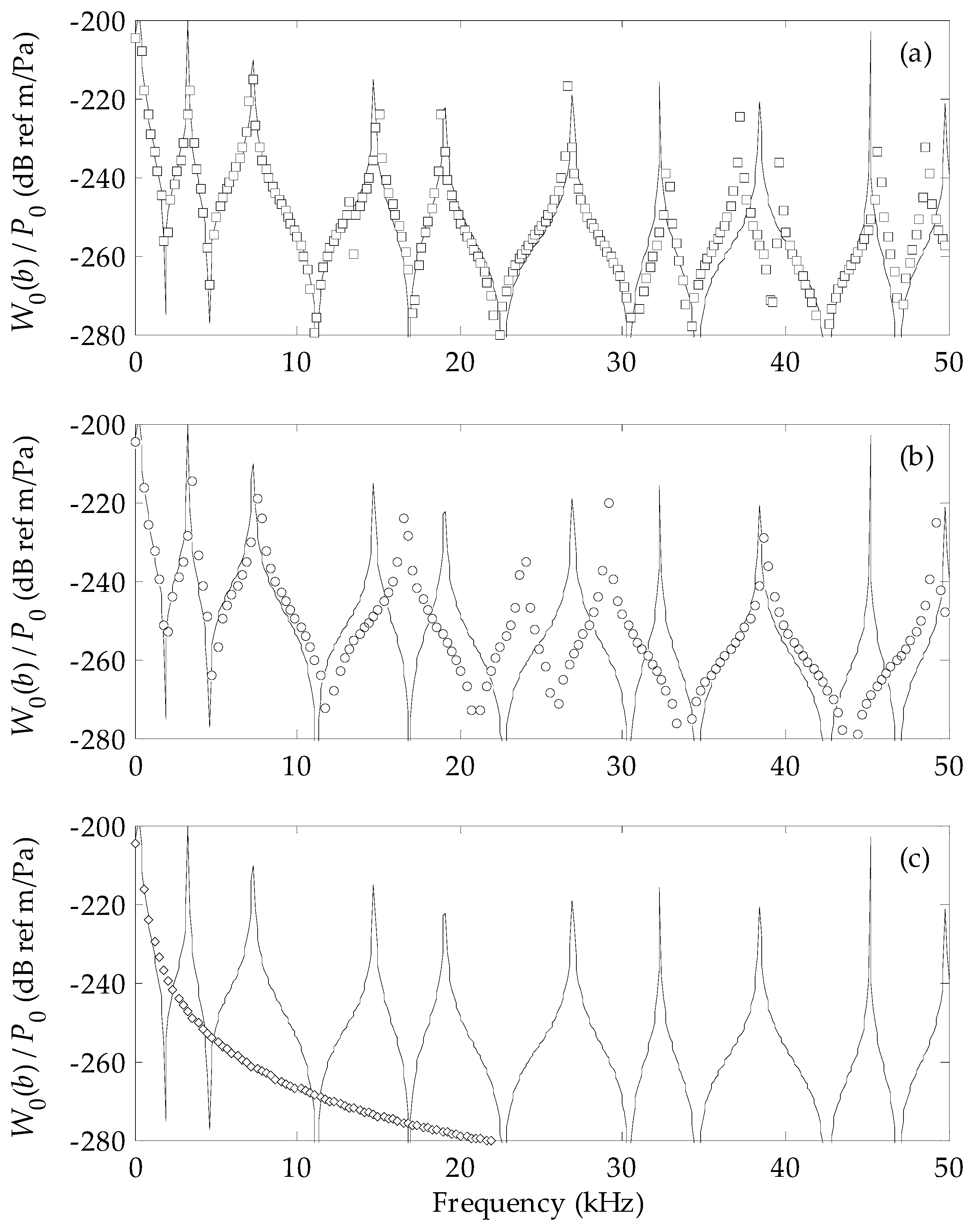
Acoustics 01 00017 g005
Figure 6. Comparison of analytical model (solid line) to finite element model (square markers) for radial displacement divided by radial pressure versus frequency for the n = 3 mode.
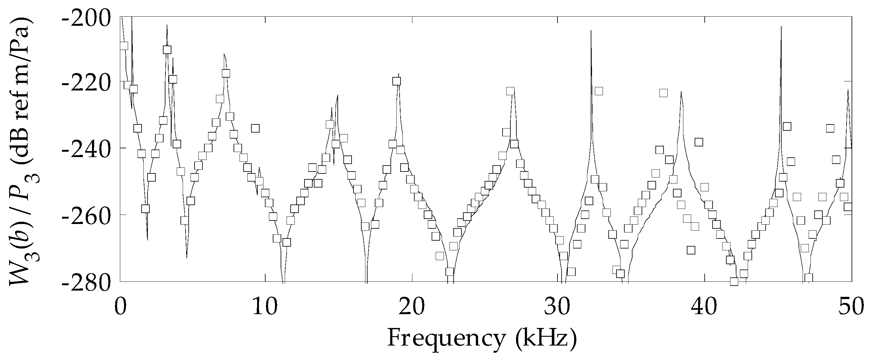
Acoustics 01 00017 g006
Figure 7. Comparison of analytical model (solid line) to finite element model (square markers) for tangential displacement divided by tangential pressure versus frequency for the n = 3 mode.
Acoustics 01 00017 g007
Figure 8. Comparison of analytical model (solid line) to finite element model (square markers) for tangential displacement divided by radial pressure (or equivalently radial displacement divided by tangential pressure) versus frequency for the n = 3 mode.
Acoustics 01 00017 g008

