Numerical Prediction of Far-Field Combustion Noise from Aeronautical Engines

Abstract

A hybrid methodology combining a detailed Large Eddy Simulation of a combustion chamber sector, an analytical propagation model of the extracted acoustic and entropy waves at the combustor exit through the turbine stages, and a far-field acoustic propagation through a variable exhaust temperature field was shown to predict far-field combustion noise from helicopter and aircraft propulsion systems accurately for the first time. For the single-stream turboshaft engine, the validation was achieved from engine core to the turbine exit. Propagation to the far field was then performed through a modeled axisymmetric jet. Its temperature modified the acoustic propagation of combustion noise significantly and a simple analytical model based on the Snell–Descarte law was shown to predict the directivity for axisymmetric single jet exhaust accurately. Good agreement with measured far-field spectra for all turboshaft-engine regimes below 2 kHz stresses that combustion noise is most likely the dominant noise source at low frequencies in such engines. For the more complex dual-stream turbofan engine, two regime computations showed that direct noise is mostly generated by the unsteady flame dynamics and the indirect combustion noise by the temperature stratification induced by the dilution holes in the combustion chamber, as found previously in the turboshaft case. However, in the turboengine, direct noise was found dominant at the combustor exit for the low power case and equivalent contributions of both combustion noise sources for the high power case. The propagation to the far-field was achieved through the temperature field provided by a Reynolds-Averaged Navier–Stokes simulation. Good agreement with measured spectra was also found at low frequencies for the low power turboengine case. At high power, however, turboengine jet noise overcomes combustion noise at low frequencies.

1. Introduction

Future aeroengines must be designed to limit cruising speed consumption, pollutant emissions and noise at landing and takeoff phases. With the development of new low NOx-emission combustion chambers, such as lean premixed, rich-quench-lean or staged-injection combustion chambers, combustion noise is becoming a significant contributor to the overall aircraft noise and, therefore, the focus of many recent studies [1,2,3,4,5,6]. The latter show that two mechanisms creating combustion noise must be distinguished: direct and indirect noise. The first one is directly related to the flame dynamics, e.g., the fluctuations of the heat release rate, which correspond to unsteady volumetric expansion generating sound waves in the reactive zone [7]. The second one is the generation of sound when entropy waves (hot and cold spots generated in the flame zone), convected by the mean flow, reach zones with significant mean flow gradients, typically a turbine blade passage [8,9]. This last source (excess noise) is thought to be important at low frequencies and was experimentally evidenced only recently by Bake et al. [10] in the Entropy Wave Generator experiment. The significant contribution of indirect noise was shown numerically and analytically by Leyko et al. [11,12,13], Duran et al. [14,15,16], Giauque et al. [17,18], and Lourier et al. [19] in nozzles, and more recently by Livebardon et al. [20] in a full engine context.

To account for these mechanisms and predict aeronautical combustor noise which propagates from the engine core to the far-field, different methodologies have been developed. As recently reviewed by Hultgren [21], most existing combustion-noise predictions for complete engines still rely on semi-empirical models. In fact, although unsteady Computational Fluid Dynamics (CFD) methods such as Large Eddy Simulation (LES) or Direct Numerical Simulation (DNS) can directly provide the acoustic field radiated by noise sources, their computational cost is high, thus they are limited to small domains close to the sources making such an approach unrealistic for core noise. Hybrid methods have been developed to overcome this limitation. In these approaches, a detailed turbulent reactive LES is used only for the noise sources in the chamber. It provides waves which are then propagated through the turbine stages with a simplified acoustically compact method taking into account that combustion noise is in the low frequency range (0–1500 Hz). These methods are analytical extensions of the methods of Cumpsty and Marble [9], the limits of which were extensively studied by Leyko et al. [22,23] through a stator vane, Wang et al. [24] through a rotor blade, and more recently by Bauerheim et al. [25] through a two-dimensional stage. The extension to a three-dimensional transonic turbine stage was also studied by Wang et al. [26] and Papadogiannis et al. [27]. Provided the attenuation of entropy waves by the mean flow is accounted for, these analytical models have been shown to propagate the waves correctly through blade rows in the frequency range of combustion noise. Similar results was recently found by Zheng et al. [28]. These first two steps correspond to the so-called CONOCHAIN (COmbustion NOise CHAIN) methodology recently developed at Cerfacs [20]. CONOCHAIN has been tested in the framework of the Turboshaft Engine Exhaust Noise Identication (TEENI) European project, showing promising results for the pressure at the turbine exit [20].

The present paper focuses on the extension of CONOCHAIN to the far-field propagation where most experimental data are available. Preliminary results were presented at two AIAA/CEAS Aeroacoustics conferences [29,30]. Computation of the resulting acoustic far-field is based on Phillips’ analogy [31] for cases where the jet velocity is low, and thus jet noise is negligible and the zero Mach-number assumption can be used. The complete methodology is presented in Section 2. Two industrial cases corresponding to turboshaft and turboengine applications, respectively, are described in Section 3. CONOCHAIN results are shown in Section 4. The TEENI turboshaft case was used as a validation case. Then, a different configuration of an industrial turbofan was studied in details to stress the robustness of the method. Conclusions are finally drawn in Section 5 and the impact of the engine architecture on combustion noise is deduced.

2. Combustion Noise Prediction

The method used to predict far-field engine combustion noise consists of three chained steps: first a LES within the chamber (Section 2.1), then the propagation of direct noise and generation of indirect noise in the turbines by the so-called CHORUS code (Section 2.2) and finally the noise propagation from the engine outlet to the far field (Section 2.3). Figure 1 shows an overview of the extended CONOCHAIN procedure.

2.1. Large Eddy Simulation of Confined Reactive Flows

The calculation of combustion noise sources requires a proper estimate of the turbulent flow to resolve velocity gradients and accelerations as well as flame dynamics. To achieve this goal, a LES is performed with the massively-parallel unstructured LES solver AVBP [32]. The latter solves the compressible Navier–Stokes equations in three-dimensional complex geometries [33] with a finite volume method and a Two-step Taylor–Galerkin numerical Scheme (TTGC) that is third-order accurate in space and time [34] to limit dispersion and dissipation. To achieve stability, Colin’s sensor is used locally to apply artificial viscosity in zones with strong gradients [35]. The sub-grid scale stresses are provided by the Smagorinsky model [36] and the flame-turbulence interactions are described by the Dynamic Thickened Flame (DTF) approach [33,35,37]. Kerosene/air chemistry is modeled using a synthetic surrogate described by a reduced mechanism involving six species and two reactions [38]. Reaction rates are modeled by Arrhenius laws [33], where the preexponential constants are fitted in rich regimes to recover proper laminar flame speeds. Non-reflective Navier–Stokes Characteristic Boundary Conditions (NSCBC) are used at inlets and outlets to limit acoustic reflections [39,40].

2.2. Direct and Indirect Noise Generation and Propagation through Turbine Blades (CHORUS)

Once the LES is statistically converged and enough fields are available, they are used to extract waves that propagate through the turbine stages. Flow variables are extracted from the LES at several planes perpendicular to the engine axis at the exit of the combustion chamber (Figure 1). By subtracting the mean flow, the entropy fluctuation, $s^{\prime }$, the velocity magnitude fluctuation, $w^{\prime }$, the pressure fluctuation, $p^{\prime }$ and the flow angle fluctuation, and ${\theta }^{\prime }$ are obtained respectively, which then yield the primitive dimensionless fluctuating variables used in Cumpsty and Marble’s model [9]:

• entropy ($s^{\prime }/C_p$)
• velocity magnitude ($w^{\prime }/c$)
• pressure ($p^{\prime }/\gamma p$)
• flow angle (${\theta }^{\prime }$)

where $\gamma$ is the specific heat ratio, p is the mean pressure, $c_p$ is the specific heat at constant pressure and c is the mean sound speed. By assuming time harmonic fluctuations, these primitive variables are combined to build upstream and downstream propagating acoustic waves (${\mathrm{w}}^{+}$ and ${\mathrm{w}}^{-}$), entropy waves (${\mathrm{w}}^s$) and vorticity waves (${\mathrm{w}}^v$). Thus, each wave $\varphi$ is written as follows,

$${\mathrm{w}}^{\varphi }=\left|{\mathrm{w}}^{\varphi }\right|exp\left(\mathrm{i}\left(\omega t-k^{\varphi }(xcos{\nu }^{\varphi }+ysin{\nu }^{\varphi })\right)\right),\forall \varphi =+,-,s,v$$

(1)

where $(x,y)$ are the coordinate systems of the turbine-blade cascades (x being the engine axis), t is the time, $\omega$ is the angular frequency, $k^{\varphi }$ is the modulus of the wave vector of the wave, and ${\nu }^{\varphi }$ is the wave front angle with respect to the engine axis, as shown in Figure 2.

The whole process can be summarized by the following steps [41,42,43]:

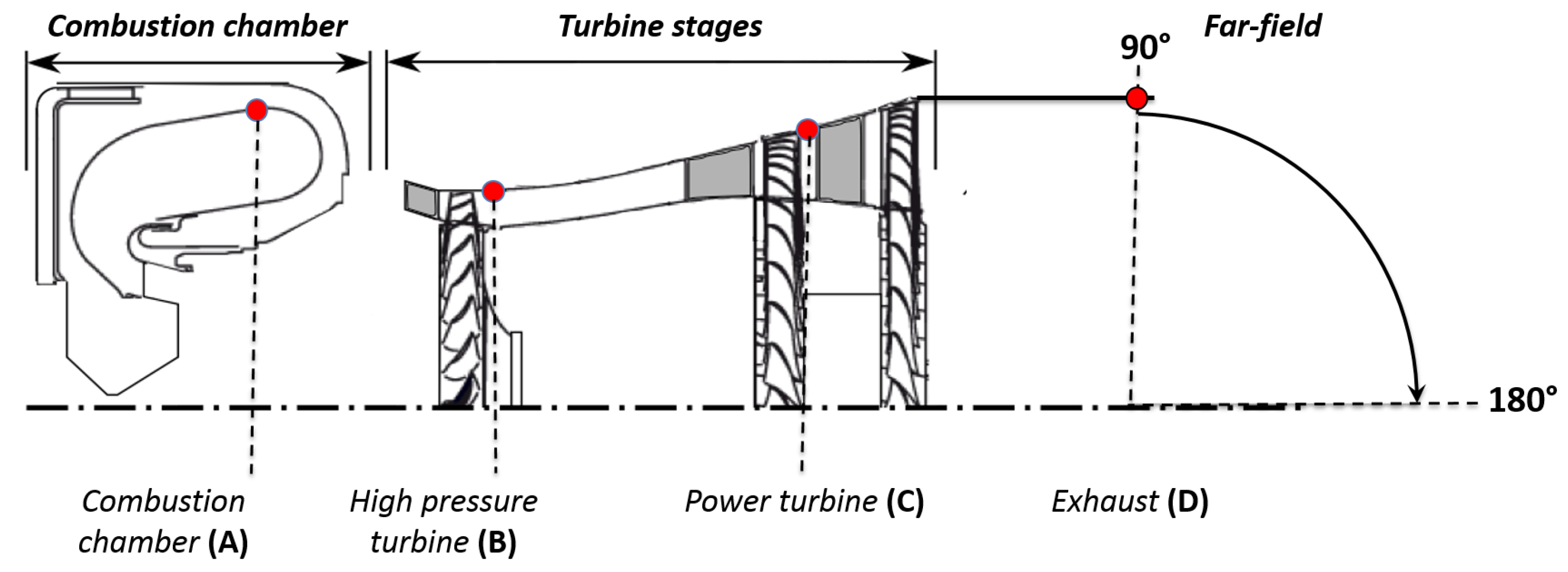
• Instantaneous LES solutions are interpolated over $N_{planes}$ planes (up to a thousand) at the outlet of the combustion chamber, as shown in Figure 1. Primitive variables are radially averaged and decomposed using temporal Fourier transform. Spatial Fourier transforms over the azimuthal direction allow performing an azimuthal modal decomposition (see Livebardon et al. for details [5]).
• Dispersion relations, derived from two-dimensional linearized Euler equations, allow building primitive variables in a waveform (Equations (10) and (11) in [5]).
• The waves ${\mathrm{w}}^{\varphi }$ are filtered at the exit of the combustion chamber using the set of $N_{planes}$ interpolating planes to extract the propagating components [44], namely

  $${\widehat{\mathrm{w}}}^{\varphi }=\frac{1}{N_{planes}}\sum _{i=1}^{N_{planes}}{\mathrm{w}}_i^{\varphi }exp\left(-\mathrm{i}{k}_x^{\varphi }{x}_i\right).$$

  (2)

  where $k_x^{\varphi }$ is the projection of the wavenumber on the engine axis and $x_i$ are the axial position of the extraction planes. The azimuthal wave numbers are obtained by spatial Fourier transform and the axial wave numbers are derived from the above dispersion relations.
• Using this wave decomposition and an extension of the actuator disk theory [9], CHORUS propagates these waves through turbine stages and computes acoustic power attributed to direct and indirect combustion noise at several locations in a real turbine.

Cumpsty and Marble’s actuator disk model [9] assumes the blade rows are compact. This requires the axial chord of each row to be lower than the acoustic wavelength so that each blade row can be seen as a thin interface. Although it limits the model to low frequencies, it is suited to our case, since combustion noise is a low frequency broadband noise (less than 1500 Hz). In a real turbofan-engine turbine, the blade axial chord is small (about 3 cm in general) compared with the acoustic wavelengths of combustion noise (40 cm at 1000 K, considering the usual maximum frequency of combustion noise, 1500 Hz, and more than 6 m at 100 Hz). In the first transonic stage of the high-pressure turbine that is relevant to indirect combustion noise, the blade axial chord also remains small compared to the entropy wavelength [27].

Matching conditions can be written between the inlet and the outlet of successive blade rows. For a stator, the conservation equations of mass $\dot{m}$, entropy $s/C_p$ and stagnation temperature $T_t$ through a stator are used. Conservation of stagnation temperature is replaced by the conservation of rothalpy $I_t$ for rotors [25]. A last relationship depends on the mean flow state at the trailing edge of the blade. For a subsonic flow, a Kutta condition is used and replaced for choked flow by the conservation of the mass-flow rate through a one-dimensional isentropic choked nozzle. To account for the propagation in the inter-blade regions, a phase shift based on the wave travel times between rows is taken into account. Although stators and rotors are assumed compact, these travel times between rotors and stators make the formulation frequency dependent. The limits of validations of this model have been assessed for a stator and a stator–rotor (stage) case [1,22,25,41,42]. Using fully unsteady simulations with AVBP, Leyko et al., Duran et al. and Bauerheim et al. showed that the planar entropy wave is not conserved through a row [22,25,41]: turbulent mixing, combined with the acceleration and deviation induced by the turbine blades, leads to a scattering of planar entropy waves through each passage so that energy is redistributed into other azimuthal modes [20,22]. The mean axial velocity profile through the turbine stage was found to be the dominant effect of this wave dispersion mechanism [22,25]. Therefore, an attenuation function of the longitudinal entropy wave has been implemented [41,45]. Bauerheim proposed a simple analytical model for the mean axial velocity profile through the turbine stage based on its asymmetry and flatness [25]. It then yields an analytical expression for the time-delay within the blade passage that can be easily integrated to provide the attenuation function. Such a procedure shows that, at low frequency, only the mean velocity deficit within the passage is important, while, at higher frequencies, an accurate velocity profile in the blade boundary layers is required. For simplicity here, the numerical attenuation function derived by Bauerheim et al. is used for all considered blade rows [25].

A second issue is the interaction between burners in a multi-burner engine as found in most gas turbines. Livebardon et al. showed that the entropy mode produced by a full combustor was not the same as the mode produced by a single sector [20]: interferences between burners decrease the overall signal level. Since no correlation between sectors appears in the full 360${}^{\circ }$ combustor LES of the TEENI engine, a filter allows to consider a random phase distribution of the planar modes of a single sector to mimic a full-annular mode. This filter function is used here for all cases if not mentioned otherwise.

2.3. Far Field Propagation through a Real Nozzle to the Atmosphere

In most cases, experimental data on engine noise are only available in the far-field. Therefore, waves obtained by CHORUS need to be propagated through the engine nozzle to the atmosphere to be compared with experimental data. This requires computing acoustic propagation through a jet of hot gases. Using Phillips’ acoustic analogy [31] allows taking into account the variation of sound speed and thus to have inhomogeneous temperature and density fields. A time Fourier transform of the resulting wave equation yields the following Helmholtz equation:

$${\displaystyle \frac{\partial }{\partial x_i}}\left(c^2{\displaystyle \frac{\partial \widehat{p}}{\partial x_i}}\right)+{\omega }^2\widehat{p}=-\mathrm{i}\omega (\gamma -1){\widehat{\dot{\omega }}}_T.$$

(3)

where $\widehat{p}$ is the harmonic acoustic pressure fluctuation, and ${\widehat{\dot{\omega }}}_T$ is the main acoustic source term related to the unsteady heat release.

Equation (3) is limited to low Mach number flows, which is the case for the two low-power applications considered here (average jet Mach number at the nozzle exit $M_j<0.3$). Moreover, there is no reactive flow at the outlet of the nozzle for the considered operating conditions (no post-combustion). Thus, ${\widehat{\dot{\omega }}}_T=0$, and Equation (3) becomes the following eigenvalue problem:

$$(\nabla .c^2\nabla +{\omega }^{2}I)\widehat{p}=0.$$

(4)

This linear system is solved by the Generalized Minimum RESidual (GMRES) method that can deal with large, sparse and non-Hermitian linear systems and belongs to the class of Krylov-based iterative methods. It allows using only Matrix-vector products. The resulting Helmholtz solver developed at Cerfacs is called AVSP [46,47].

As shown in Figure 1, the waves obtained at the outlet of the turbines are then injected into the forced version of the above Helmholtz solver AVSP-f [48]. This forcing is performed at the turbine exit, where the incoming acoustic wave $A^{+}=p^{\prime }+\rho c{u}^{\prime }$ is injected through an acoustically non-reflecting inlet. The corresponding wave amplitude $\widehat{p}$ is imposed as a function of frequency $f=\omega /\left(2\pi \right)$ at each node of the surface.

3. Industrial Configurations and Experimental Measurements

3.1. TEENI: A Full-Scale Experimental Test

The first experimental system was a fully instrumented helicopter engine for which both far field and chamber turbine measurements of pressure levels were performed during the TEENI project [49]. As such, it constitutes a unique experimental engine database for core noise. The actual experimental set-up is shown in Figure 3.

Unsteady pressures were measured in the far field and within the turbine at the locations shown in Figure 4 (in the combustion chamber (A), in the high-pressure turbine (B), in the power turbine (C) and at the exhaust (D)) for seven different operating points from the lowest power setting encountered in flight conditions to take-off power. Note that only two azimuthal pressure probes were available within the engine [5]. The CONOCHAIN methodology presented in Section 2 was applied to the actual experimental configuration to evaluate its ability to predict the combustion noise generated by a helicopter engine. Two operating points corresponding to low and high powers were numerically investigated thus far [5]. For both engine conditions, Liverbardon et al. showed good agreement between the pressure measurements and the simulation results not only in the combustion chamber but also after the different blade rows of the TEENI engine, as shown in Figure 4 [5].

This turboshaft configuration is also interesting because there is no significant jet noise (low exhaust jet velocity), thus experimental data obtained for far field noise mainly consist of combustion noise and can be used for validation.

3.2. An Industrial Turbofan Engine

The second configuration was an annular burner of a turbofan engine, termed engine B, composed of identical injectors placed periodically. Here, the computational domain was a single sector of the chamber with only one injector (Figure 5), followed by the High Pressure Turbine Stator (HPTS). Each sector was divided into three parts:

• An injector with two corotative swirlers
• A by-pass duct
• The flame tube

To study combustion noise, the first operating point corresponded to a low power regime used for taxiing. For this operating condition, the jet velocity is low (<100 m/s) and jet noise is negligible. The second operating point was the full power case, corresponding to take-off conditions.

Table 1. Main characteristics of the operating points used for the LES simulations.

	Low	Full
Inlet pressure ratio	12%	100%
Temperature ratio	54%	100%
Air mass-flow rate ratio	13%	100%
Fuel mass-flow rate ratio	9%	100%
Fuel/Air ratio	1.2446	1.92

summarizes both engine conditions. All parameters were normalized by the corresponding full power conditions.

The turbojet engine chamber is followed by two turbines (Figure 5). The first one is a high pressure turbine (HPT) composed of one stator and one rotor, i.e., one single stage. The last one is a low pressure turbine (LPT) composed of three stages. For both operating points, the turbines have different characteristics, as summarized in

Table 2. Characteristics of the high-pressure (HPT) and low-pressure (LPT) turbines for both operating points.

		Low	Full
HPT	Dimensionless rotational speed	62%	100%
	Inlet Pressure ratio	100%	100%
	Inlet Temperature ratio	100%	100%
	Outlet Pressure ratio	59%	31%
	Outlet Temperature ratio	79%	70%
LPT	Dimensionless rotational speed	22%	100%
	Inlet Pressure ratio	53%	26%
	Inlet Temperature ratio	75%	68%
	Outlet Temperature ratio	73%	53%

. The rotational speeds are normalized by the full power-case speed, while pressure and temperature are divided by the inlet conditions of the high pressure turbine.

The robustness of the combustion noise prediction method was tested by comparing results with acoustic pressure data obtained in the far field from the engine test bench. Aft noise measurements were achieved at 45 m with an acoustic barrier shielding noise from the inlet.

4. CONOCHAIN Results

4.1. TEENI Case

The global CONOCHAIN tool was first applied to the TEENI industrial turboshaft-engine case (Section 3.1). Only the high-power condition was considered here as it represents the most challenging and relevant case to meet acoustic specifications. Details and validation of the combustion-chamber LES for both engine configurations were provided by Liverbardon et al. [5]. Results were first compared with pressure fluctuations measured in the turbine stages representative of the internal noise sources, because, as mentioned above, the TEENI project provided unique measurements within the engine in addition to far-field noise [5]. Finally, acoustic propagation to the far-field (19 m away from the engine exhaust) was investigated.

4.1.1. Acoustic Activity from the Chamber to the Engine Exhaust

The unsteady analysis of LES results provided the amplitudes of acoustic and entropy waves responsible for direct and indirect combustion noise. The first step was to compare LES and experimental results within the flame tube itself (Figure 1). In the chamber, only direct noise contributes to total noise since entropy waves have not yet been accelerated significantly through the high pressure turbine. This was verified by Liverbardon et al. by showing high coherence levels between the heat release within the combustion chamber and the pressure fluctuations at the combustor exhaust [5]. Figure 6a shows a good agreement between the experimental Power Spectral Densities (PSD) of pressure fluctuations and the numerical results in terms of broadband levels and spectral shape. The experimental oscillations were caused by the design and the response of the remote microphone probes (RMP) [5].

By splitting acoustic and convective waves at the exit of the combustion chamber, CONOCHAIN allows computing the contribution of direct and indirect combustion noise within the turbine stages. Propagation of noise sources through the high pressure turbine, the power turbine and up to the engine exhaust was investigated with the analytical method described in Section 2.2. Extreme pressure spectra obtained from the two azimuthal microphones delimit a grey zone that provides an estimate of the experimental uncertainty and stresses the circumferential asymmetry in the actual engine. In these spectra, the tonal peaks are generated by the rotating shafts and correspond to the turbine blade passing frequencies: turbine noise is therefore seen from 600 Hz. Using a three-sensor technique, Liverbardon et al. also showed that a significant narrow component of direct combustion noise was found around 200 Hz generated in the combustion chamber, and that a broadband hump up to 1200 Hz could be attributed to broadband noise generated by the HPT, which could be indirect combustion noise [5]. These experimental spectra were compared with the spectra obtained from the combustion waves (Figure 6b–d) at each position defined in Figure 4. In the low frequency range where CONOCHAIN is valid (typically less than 1 kHz), the predicted values capture both the experimental trend and levels, as already found by Liverbardon et al. [5]. They also showed similar good results at low power, which suggests that combustion noise is the dominant source at low frequencies for all turboshaft-engine regimes. Possible explanations for the remaining discrepancies are the drastic simplification of the geometry in the analytical propagation models, additional noise sources (including the evidenced turbine noise) that may also occur locally in the engine near the pressure probe, and the experimental uncertainty that is only indicative due to the lack of in-situ calibration for instance.

4.1.2. Analysis of the the Far-Field Acoustic Pressure

When acoustic waves were identified at the engine outlet (Position D in Figure 4a), they were used to force the ingoing waves in the AVSP-f computation of the propagation to the far field. As explained in Section 2.3, the injection of waves was done through an inlet NSCBC boundary condition. The total acoustic contribution (direct and indirect noise) was used here for this forcing.

The hot jet of a turboshaft engine, which is single stream and axisymmetric, has temperature inhomogeneities. Phillips’ analogy assumes inhomogeneities in the mean flow. Thus, sound speed variations can be considered and this allows describing an inhomogeneous temperature field corresponding to a jet flow of a subsonic nozzle. As no flow simulation of TEENI engine exhaust was possible (no available nozzle geometry), the temperature field of the jet was evaluated using the correlation of Zaman [50] and Pope [51] for turbulent jets, as summarized in Appendix A.

To first investigate the impact of the temperature on the propagation of waves, zero Mach-number AVSP simulations were made with the same amplitude of 100 Pa imposed for different frequencies from 0 to 1000 Hz, and two different initializations of the mean field. On the one hand, an isothermal field (300 K) was imposed in the whole computational domain; on the other hand, the non-uniform mean field was obtained from the above simplified jet model. As shown in Figure 7, the temperature field has a major impact on the directivity of the acoustic field. For the isothermal field the maximum directivity of combustion noise measured from the engine axis is in the jet direction (${180}^{\circ }$ in Figure 4), whereas the maximum directivity is shifted between ${130}^{\circ }$ and ${140}^{\circ }$ for the stratified field. In fact, the plane wave is refracted within the jet because of the change of medium, and the different sound speeds between the hot potential core and the cold shear layer and external flow. A simple model based on the Snell–Descarte law is proposed in Appendix B to explain this particular directivity of combustion noise.

The same methodology was then applied to the actual TEENI high-power configuration. The PSD of the far-field acoustic pressure around the maximum directivity angle were compared with the experimental data available at 19 m in Figure 8. A good agreement was found between the experimental PSD of acoustic pressure and the numerical results in terms of broadband levels and patterns. Similar good results were obtained at low power, confirming that combustion noise is indeed the dominant source at low frequencies for all turboshaft-engine regimes [52]. Possible explanations for the remaining discrepancies are the above uncertainty on the source levels at the exhaust, the drastic simplification of the jet that has most likely a different potential core, and the possible contribution from low-order azimuthal modes that are neglected in the current one-burner sector simulations [20]. Moreover, low Mach number convection effects (neglected here) can still slightly modify the combustion noise directivity near the axis, as recently shown by Ferand et al. [30] (see below).

4.2. Engine B Case

4.2.1. Single-Sector LES of the Combustion Chamber

LES of a single sector was first run for 48 ms of physical time with a time-step of $3\times {10}^{-8}$ s respecting a maximum CFL number of 0.7. Fuel was injected in gaseous phase close to the lips of the swirler to mimic the fast evaporation of the kerosene spray. A cold flow was injected in the by-pass duct and around the walls by inlet films and multiperforated plates, to cool the chamber walls. Multiperforated plates were modeled by a homogeneous plate with a specific effusion condition [53]. For both simulations (low and full power), the HPTS was choked, and no additional boundary condition was needed at the chamber outlet (Figure 9). All walls of the chamber were defined as adiabatic with a turbulent wall-law model to evaluate and impose the wall-shear stress.

The geometry was discretized with tetrahedral elements (

Table 3. Mesh parameters.

Number of cells	33,134,438
Number of nodes	6,199,870
Smallest volume	$2.3\times {10}^{-14}$ m${}^3$
Time step	$3\times {10}^{-8}$ s

) and a fine discretization around the injection system and the flame was used to capture small geometrical details and physics.

Mean velocity fields for both engine configurations are presented in Figure 10 in a meridional plane of the combustion chamber, and scaled by the inlet mean velocity $U_{inlet}$ of the full power case. In both cases, the expected formation of the precessing vortex core was evidenced at the swirler lips with large recirculation zones in the center of the combustion chamber [54]. This swirling flow was mixed with the secondary flows coming from the dilution holes and a radially-stratified velocity field was then sucked into the turbine.

The dimensionless mean temperature fields for both engine configurations are represented in Figure 11a,b in a meridional plane of the combustion chamber, and in Figure 11c,d in a midspan blade-to-blade surface through the HPTS vanes, respectively. They correspond to ${\displaystyle \frac{T-T_{inlet}}{T_{adiab}-T_{inlet}}}$, where $T_{inlet}$ is the mean inlet temperature and $T_{adiab}$ is the mean adiabatic temperature. The mean flame location is highlighted by the iso-lines of the mean heat-release. The most reactive zones were confined close the swirler but there was also a reacting zone near the dilution holes for both power conditions. The mean temperature fields were characterized by a primary zone in which combustion took place to reach the adiabatic temperature for both simulations. To reduce the mean temperature before the high pressure turbine, air flow was injected from the dilution holes and interacted with the burnt gases. This created the strong temperature stratification both radially (Figure 11a,b) and azimuthally (Figure 11c,d) that was then sucked by the HPTS and yielded strong indirect combustion noise, as already seen in the TEENI case [5].

The root-mean-squared (RMS) pressure fields are shown in Figure 12 for both engine configurations in a meridional plane of the combustion chamber. In both cases, the main pressure fluctuations were located close to the swirler and the interaction zones induced by the dilution-hole cross-flow jets. As expected in terms of fluctuating pressure levels, the low power simulation showed far less activity than the higher operating point, which had levels of fluctuations ten times higher than the lower one.

The corresponding root-mean-squared (RMS) temperature fields (Figure 13) reveal two main zones of fluctuating temperature. First, in the primary zone, temperature fluctuations corresponded to the shape of the turbulent flame where turbulent structures interacted with the flame front, which convected fresh gases across the reacting zone. Second, the interaction of the dilution jet flows at the end of the primary zone generated the strongest temperature fluctuations in both cases, as highlighted in Figure 14. Both contributed to direct combustion noise. The instantaneous fluctuating temperature contours also showed that the largest hot spots responsible for indirect combustion noise in the HPT were generated in the second half of the flame tube.

Fluctuations of acoustic pressure and entropy were extracted on planes P located one chord before the HPTS, as shown in Figure 15 and explained in Section 2.2. The PSDs of the acoustic pressure fluctuations at the outlet of the combustion chamber are illustrated in Figure 16 for both engine regimes. A bump around 500 Hz was observed at low power and was still present at full power condition, even if a slight shift in frequency was seen. As expected, the broadband pressure-fluctuation level increased with power rating.

4.2.2. Acoustic Power in the Turbine Stages

Acoustic and entropy waves were propagated through the turbine stages with CHORUS to yield the distribution of direct and indirect noise at the outlet of each row of the turbine (Figure 17). Figure 17a shows this distribution for the taxi out operating point (low power), whereas Figure 17b provides the distribution for the full power conditions. Contrary to the turboshaft case, very different behaviors were obtained for the two engine regimes of the turbofan. Direct combustion noise is clearly the dominant mechanism in the low power case. At full power conditions, the dominant mechanism between indirect and direct noise can no longer be identified. Indirect noise is much more present for this operating point than at low power.

At low power, when comparing the spectra between the combustion chamber (Figure 16) and the outlet of the turbine (Figure 18a), the spectral shape was seen to be globally conserved for both combustion-noise sources between the chamber and the outlet of the turbine. The spectra were broadband with a bump at 500 Hz, even if this hump was less pronounced for indirect noise. Only power losses occurred through the turbine stages. In a full-annular combustor, the overall signal level of indirect noise is decreased since there are no correlations between the entropy planar mode of each sector. Whereas the introduced filter did not change the hierarchy of sources in the turboshaft case, the contribution of indirect noise in the turbofan case changed, and the direct noise became dominant. In the high power case, the power losses through the turbine stages were less important and the spectral shape was modified for both combustion-noise sources by the transmission through the turbine stages, as shown in Figure 18b. This can be explained by the different flow angles at each turbine stage for the engine regime, as shown by Leyko et al. (Figure 4 in [22]).

4.2.3. Analysis of the Far-Field Acoustic Pressure

In the actual turbofan engine, the jet is a dual stream with an internal lobe mixer and consequently has temperature inhomogeneities. However, to simplify the geometry, the mixer was replaced by a primary nozzle, which gives similar flow conditions. Because of the complex dual-stream jet, the simple jet-flow model in Appendix A cannot be used to initialize the AVSP-f computations. Instead, Reynolds-Averaged Navier–Stokes (RANS) simulations were performed on a hybrid grid resolving the boundary layers with prisms in the nozzle, using ANSYS-FLUENT v.15 [55]. A standard k–$\epsilon$ model was used for the turbulence closure, and high-order schemes were applied to discretize the RANS equations. The resulting field of speed of sound normalized by its maximum value in each engine regime is shown in Figure 19. The top part of the plot corresponds to the flow solution of the low power engine regime, whereas the bottom part corresponds to that of the high power engine regime, as described in Section 3.2. The lengths of the potential core are almost the same (white arrow) but the spreading of the jet is clearly different in both regimes yielding different temperature and speed of sound fields.

The acoustic computational domain is represented in Figure 20. Since a single sector of combustor was computed, only plane waves are meaningful. By considering low frequency (<2000 Hz) plane modes, the computational domain can be reduced to a slice of the atmosphere. To have a good resolution up to 2000 Hz (${\lambda }_{2000\mathrm{Hz}}=17.2$ cm), ten nodes per wavelength are approximately needed, which limits the possible far-field range directly solved with the Helmholtz solver AVSP-f. The latter then provided the modulus and phase of the acoustic pressure up to 7.5 m from ${90}^{\circ }$ to ${180}^{\circ }$. To obtain the measured pressure levels in the far-field, this acoustic pressure obtained at 7.5 m was then propagated up to 45 m, assuming a monopolar radiation and a spherical wave propagation.

In Figure 21, the computed far-field combustion noise is compared with the measured turbofan sound pressure levels at 45 m. The grey areas stand for the experimental variation of different tests around the simulated engine regime, and the uncertainty of the microphone measurements. At low power, jet velocity is low, thus jet noise is negligible. Consequently, combustion noise is the main noise source at low frequency: the spectral content was well predicted and the correct order of magnitude was captured. This confirmed the results of Livebardon et al. [5] in the TEENI turboshaft case but for a more complex dual-stream turbofan case. Spectra are broadband with one tone around 500 Hz, as observed before in the combustion chamber (Figure 16) and in the turbine (Figure 17). However, a slight shift of the bump frequency can be observed between the simulation and the experimental data. The spectrum would most likely need more frequency resolution to correctly identify the localization of the tone.

Figure 22 shows the overall sound directivity measured in the far field at 45.72 m from the engine exhaust (solid line) for the angles defined in Figure 4. The prediction of the present CONOCHAIN methodology is shown with solid circles and compares favorably with experiment, stressing the importance of accounting for the actual jet temperature. However, the maximum sound level is found at about ${150}^{\circ }$ (grey arrow) compared to about ${140}^{\circ }$ in the measurements. Ferand et al. [30] recently performed two LES of the actual jet flow with (solid squares) and without (solid triangles) combustion noise forcing. In the latter, the turbulent jet noise levels are found negligible, consistently with the low exhaust velocity. The forcing case termed FJBSC is very close to the CONOCHAIN result, stressing the dominant contribution of combustion noise at low engine power, and in good agreement with the measurements at least up to ${130}^{\circ }$, with a maximum discrepancy of about 5 dB at ${90}^{\circ }$. The maximum sound level at ${140}^{\circ }$ (black arrow) is recovered, stressing that there is a little convection effect along the jet axis in this engine case, even at low engine power.

At high power (Figure 21), the noise spectrum is still broadband but with a maximum of radiation at 150 Hz. A sharper decrease is observed in the simulation between 500 and 2000 Hz than in the experimental total engine-noise spectra (in Figure 21b particularly). At full power, jet noise is becoming the dominant noise source compared with combustion noise [30]. Consequently, experimental sound pressure levels are higher, and additional noise sources need to be predicted for the highest engine regimes to compare with far-field turbofan bench data.

5. Conclusions

A complete hybrid methodology combining CFD methods and analytical models, termed CONOCHAIN, has been described for the prevision of far-field combustion noise from helicopter and aircraft propulsion systems for the first time. It combines a detailed LES of a combustion chamber sector, an analytical propagation model of the extracted acoustic and entropy waves at the combustor exit through the turbine stages (CHORUS), and a generalized Helmholtz propagation code through a variable temperature field (AVSP). It is worthy noting that a specific decorrelation filter is used to account for the interaction between the multiple engine burners, and an attenuation function through each turbine row is introduced to properly simulate the effect of the mean flow on the entropy waves.

Comparisons with experimental data were made for two different industrial cases: the TEENI single-stream turboshaft engine for which validations were obtained from engine core to the turbine exit, and a more complex modern dual-stream turbofan engine for which only far-field acoustic pressure was available. In the first case, the propagation to the far-field was achieved through an axisymmetric single-stream jet. As no exhaust flow simulations were available, a simple jet model has been proposed. In the second case, the propagation to the far-field was achieved through an actual dual-stream exhaust for which a RANS simulation provided the temperature field fed to AVSP. Accounting for the actual jet temperatures was shown to be key, as it significantly changes the directivity of combustion noise. A simple analytical model based on the Snell–Descarte law was actually shown to predict such a directivity for axisymmetric single jet exhaust accurately.

Good agreement was first found between CONOCHAIN combustion-noise results and measured far-field spectra for all turboshaft-engine regimes below 2 KHz, stressing that combustion noise is most likely the dominant noise source at low frequencies in such engines. Combustion noise mechanisms were then described in a realistic turboengine for two operating conditions corresponding to low and high power. As in the turboshaft, the strong stratification of temperature induced by the dilution holes is the main cause of indirect combustion noise. Direct combustion noise is rather connected to the turbulent flame unsteadiness, and possibly to its interaction with the dilution cross-flow jets. However, in the turboengine, direct noise was found dominant at the combustor exit for the low power case and equivalent contributions of both combustion noise sources for the high power case. In the turboengine case, the multi-burner filter was found to play a significant role in the combustion-noise contributions, whereas it did not alter the hierarchy in the turboshaft case. Moreover, the propagation through the turbines stages was found to be different in both turboengine regimes. For low power, the combustion noise features are essentially damped but the spectral shapes are preserved as in all turboshaft cases, whereas for the high power case both the levels and the spectral shape are altered, because of the multiple blade rows and significant different flow deviations in each of them. At high power, combustion noise was also found to be negligible compared to jet noise in the turboengine case, which can be explained by the much higher jet exhaust for this engine type compared to turboshafts.

Finally, the complete CONOCHAIN+AVSP-f hybrid method was therefore shown to accurately predict engine noise at low frequencies provided jet noise remains negligible. For instance, at high power, turboengine jet noise is seen to overcome combustion noise at low frequencies, which suggests studying the effect of combustion noise and its associated acoustic waves on jet noise.

References

1. Duran, I.; Leyko, M.; Moreau, S.; Nicoud, F.; Poinsot, T. Computing combustion noise by combining Large Eddy Simulations with analytical models for the propagation of waves through turbine blades. Comptes Rendus de l’Académie des Sciences—Mécanique 2013, 341, 131–140. [Google Scholar] [CrossRef]
2. Liu, Y.; Dowling, A.P.; Swaminathan, N.; Morvant, R.; Macquisten, M.A.; Caracciolo, L.F. Prediction of Combustion Noise for an Aeroengine Combustor. J. Prop. Power 2014, 30, 114–122. [Google Scholar] [CrossRef]
3. Dowling, A.P.; Mahmoudi, Y. Combustion noise. Proc. Combust. Inst. 2015, 35, 65–100. [Google Scholar] [CrossRef]
4. Morgans, A.S.; Duran, I. Entropy noise: A review of theory, progress and challenges. Int. J. Spray Combust. Dyn. 2016, 8, 285–298. [Google Scholar] [CrossRef]
5. Livebardon, T.; Moreau, S.; Gicquel, L.; Poinsot, T.; Bouty, E. Combining LES of combustion chamber and an actuator disk theory to predict combustion noise in a helicopter engine. Combust. Flame 2016, 165, 272–287. [Google Scholar] [CrossRef]
6. Ihme, M. Combustion and Engine-Core Noise. Ann. Rev. Fluid Mech. 2017, 49, 277–310. [Google Scholar] [CrossRef]
7. Bragg, S. Combustion noise. J. Inst. of Fuel 1963, 36, 12–16. [Google Scholar]
8. Marble, F.E.; Candel, S. Acoustic disturbances from gas nonuniformities convected through a nozzle. J. Sound Vib. 1977, 55, 225–243. [Google Scholar] [CrossRef]
9. Cumpsty, N.A.; Marble, F.E. The interaction of entropy fluctuations with turbine blade rows; a mechanism of turbojet engine noise. Proc. R. Soc. Lond. A 1977, 357, 323–344. [Google Scholar] [CrossRef]
10. Bake, F.; Richter, C.; Muhlbauer, B.; Kings, N.; Rohle, I.; Thiele, F.; Noll, B. The Entropy Wave Generator (EWG): A reference case on entropy noise. J. Sound Vib. 2009, 326, 574–598. [Google Scholar] [CrossRef]
11. Leyko, M.; Nicoud, F.; Moreau, S.; Poinsot, T. Numerical and Analytical Investigation of the Indirect Noise in a Nozzle; Center for Turbulence Research, NASA AMES, Stanford University: Stanford, CA, USA, 2008; pp. 343–354. [Google Scholar]
12. Leyko, M.; Nicoud, F.; Poinsot, T. Comparison of Direct and Indirect Combustion Noise Mechanisms in a Model Combustor. AIAA J. 2009, 47, 2709–2716. [Google Scholar] [CrossRef]
13. Leyko, M.; Moreau, S.; Nicoud, F.; Poinsot, T. Numerical and analytical investigation of the indirect combustion noise in a nozzle. Comptes Rendus Mécanique 2009, 337, 415–425. [Google Scholar] [CrossRef]
14. Duran, I.; Moreau, S. Analytical and numerical study of the Entropy Wave Generator experiment on indirect combustion noise. In Proceedings of the 17th AIAA/CEAS Aeroacoustics Conference, Portland, OR, USA, 5–8 June 2011. [Google Scholar]
15. Duran, I.; Moreau, S.; Poinsot, T. Analytical and numerical study of combustion noise through a subsonic nozzle. AIAA J. 2013, 51, 42–52. [Google Scholar] [CrossRef]
16. Duran, I.; Moreau, S. Solution of the quasi-one-dimensional linearized Euler equations using flow invariants and the Magnus expansion. J. Fluid Mech. 2013, 723, 190–231. [Google Scholar] [CrossRef]
17. Giauque, A.; Huet, M.; Clero, F. Analytical Analysis of Indirect Combustion Noise in Subcritical Nozzles. J. Eng. Gas Turbines Power 2012, 134, 111202. [Google Scholar] [CrossRef]
18. Huet, M.; Giauque, A. A nonlinear model for indirect combustion noise through a compact nozzle. J. Fluid Mech. 2013, 733, 268–301. [Google Scholar] [CrossRef]
19. Lourier, J.; Huber, A.; Noll, B.; Aigner, M. Numerical Analysis of Indirect Combustion Noise Generation Within a Subsonic Nozzle. AIAA J. 2014, 52, 2114–2126. [Google Scholar] [CrossRef]
20. Livebardon, T.; Moreau, S.; Poinsot, T.; Bouty, E. Numerical investigation of combustion noise generation in a full annular combustion chamber. In Proceedings of the 21th AIAA/CEAS Aeroacoustics Conference (36rd AIAA Aeroacoustics Conference), Dallas, TX, USA, 22–26 June 2015. [Google Scholar]
21. Hultgren, L. A Comparison of Combustor-Noise Models. In Proceedings of the 18th AIAA/CEAS Aeroacoustics Conference (33rd AIAA Aeroacoustics Conference), Colorado Springs, CO, USA, 4–6 June 2012. [Google Scholar]
22. Leyko, M.; Duran, I.; Moreau, S.; Nicoud, F.; Poinsot, T. Simulation and Modelling of the waves transmission and generation in a stator blade row in a combustion-noise framework. J. Sound Vib. 2014, 333, 6090–6106. [Google Scholar] [CrossRef]
23. Mishra, A.; Bodony, D.J. Evaluation of actuator disk theory for predicting indirect combustion noise. J. Sound Vib. 2013, 332, 821–838. [Google Scholar] [CrossRef]
24. Wang, G.; Duchaine, F.; Papadogiannis, D.; Duran, I.; Moreau, S.; Gicquel, L. An overset grid method for large eddy simulation of turbomachinery stages. J. Comput. Phys. 2014, 274, 333–355. [Google Scholar] [CrossRef]
25. Bauerheim, M.; Duran, I.; Livebardon, T.; Wang, G.; Moreau, S.; Poinsot, T. Transmission and reflection of acoustic and entropy waves through a stator–rotor stage. J. Sound Vib. 2016, 374, 260–278. [Google Scholar] [CrossRef]
26. Wang, G.; Sanjosé, M.; Moreau, S.; Papadogiannis, D.; Duchaine, F.; Gicquel, L. Noise mechanisms in a transonic high-pressure turbine stage. Int. J. Aeroacoust. 2016, 15, 144–161. [Google Scholar] [CrossRef]
27. Papadogiannis, D.; Duchaine, F.; Gicquel, L.; Wang, G.; Moreau, S.; Nicoud, F. Assessment of the indirect combustion noise generated in a transonic high-pressure turbine stage. J. Eng. Gas Turb. Power 2016, 138, 041503. [Google Scholar] [CrossRef]
28. Zheng, J.; Giauque, A.; Ducruix, S. A 2D-axisymmetric analytical model for the estimation of indirect combustion noise in nozzle flows. In Proceedings of the 21st AIAA/CEAS Aeroacoustics Conference, Dallas, TX, USA, 22–26 June 2015. [Google Scholar]
29. Ferand, M.; Livebardon, T.; Moreau, S.; Sensiau, C.; Bouty, E.; Sanjosé, M.; Poinsot, T. Numerical investigation of combustion noise from aeronautical combustor to far-field. In Proceedings of the 22nd AIAA/CEAS Aeroacoustics Conference, Lyon, France, 30 May–1 June 2016. [Google Scholar]
30. Ferand, M.; Daviller, G.; Moreau, S.; Sensiau, C.; Poinsot, T. Using LES for combustion noise propagation to the far-field by considering the jet flow of a dual-stream nozzle. In Proceedings of the 24th AIAA/CEAS Aeroacoustics Conference, Atlanta, GA, USA, 25–29 June 2018. [Google Scholar]
31. Phillips, O.M. On the generation of sound by supersonic turbulent shear layers. J. Fluid Mech. 1960, 9, 1–28. [Google Scholar] [CrossRef]
32. Schønfeld, T.; Rudgyard, M. Steady and Unsteady Flows Simulations Using the Hybrid Flow Solver AVBP. AIAA J. 1999, 37, 1378–1385. [Google Scholar] [CrossRef]
33. Poinsot, T.; Veynante, D. Theoretical and Numerical Combustion, 3rd ed.; R.T. Edwards, Inc.: Philadelphia, PA, USA, 2011. [Google Scholar]
34. Colin, O.; Rudgyard, M. Development of high-order Taylor-Galerkin schemes for unsteady calculations. J. Comput. Phys. 2000, 162, 338–371. [Google Scholar] [CrossRef]
35. Colin, O.; Ducros, F.; Veynante, D.; Poinsot, T. A thickened flame model for large eddy simulations of turbulent premixed combustion. Phys. Fluids 2000, 12, 1843–1863. [Google Scholar] [CrossRef]
36. Smagorinsky, J. General circulation experiments with the primitive equations: 1. The basic experiment. Mon. Weather Rev. 1963, 91, 99–164. [Google Scholar] [CrossRef]
37. Selle, L.; Lartigue, G.; Poinsot, T.; Koch, R.; Schildmacher, K.U.; Krebs, W.; Prade, B.; Kaufmann, P.; Veynante, D. Compressible Large-Eddy Simulation of turbulent combustion in complex geometry on unstructured meshes. Combust. Flame 2004, 137, 489–505. [Google Scholar] [CrossRef]
38. Franzelli, B.; Riber, E.; Sanjosé, M.; Poinsot, T. A two-step chemical scheme for Large-Eddy Simulation of kerosene-air flames. Combust. Flame 2010, 157, 1364–1373. [Google Scholar] [CrossRef]
39. Poinsot, T.; Lele, S. Boundary conditions for direct simulations of compressible viscous flows. J. Comput. Phys. 1992, 101, 104–129. [Google Scholar] [CrossRef]
40. Selle, L.; Nicoud, F.; Poinsot, T. The actual impedance of non-reflecting boundary conditions: implications for the computation of resonators. AIAA J. 2004, 42, 958–964. [Google Scholar] [CrossRef]
41. Leyko, M.; Moreau, S.; Nicoud, F.; Poinsot, T. Waves transmission and generation in turbine stages in a combustion-noise framework. In Proceedings of the 16th AIAA/CEAS Aeroacoustics Conference, Stockholm, Sweden, 7–9 June 2010. [Google Scholar]
42. Duran, I.; Moreau, S. Study of the attenuation of waves propagating through fixed and rotating turbine blades. In Proceedings of the 18th AIAA/CEAS Aeroacoustics Conference (33rd AIAA Aeroacoustics Conference), Colorado Springs, CO, USA, 4–6 June 2012. [Google Scholar]
43. Duran, I.; Moreau, S. Numerical simulation of acoustic and entropy waves propagating through turbine blades. In Proceedings of the 19th AIAA/CEAS Aeroacoustics Conference (34th AIAA Aeroacoustics Conference), Berlin, Germany, 27–29 May 2013. [Google Scholar]
44. Kopitz, J.; Huber, A.; Sattelmayer, T.; Polifke, W. Thermoacoustic Stability Analysis of an Annular Combustion Chamber with Acoustic Low Order Modeling and Validation Against Experiment. In Proceedings of the International Gas Turbine and Aeroengine Congress & Exposition, Reno, NV, USA, 6–9 June 2005. [Google Scholar]
45. Duran, I.; Leyko, M.; Moreau, S.; Nicoud, F.; Poinsot, T. Computing combustion noise by combining Large Eddy Simulations with analytical models for the propagation of waves through turbine blades. In Proceedings of the 3rd Colloquium INCA, Toulouse, France, 17–18 November 2011. [Google Scholar]
46. Martin, C.; Benoit, L.; Sommerer, Y.; Nicoud, F.; Poinsot, T. LES and acoustic analysis of combustion instability in a staged turbulent swirled combustor. AIAA J. 2006, 44, 741–750. [Google Scholar] [CrossRef]
47. Selle, L.; Benoit, L.; Poinsot, T.; Nicoud, F.; Krebs, W. Joint use of Compressible Large-Eddy Simulation and Helmholtz solvers for the analysis of rotating modes in an industrial swirled burner. Combust. Flame 2006, 145, 194–205. [Google Scholar] [CrossRef]
48. Silva, C.F.; Nicoud, F.; Schuller, T.; Durox, D.; Candel, S. Combining a Helmholtz solver with the flame describing function to assess combustion instability in a premixed swirled combustor. Combust. Flame 2013, 160, 1743–1754. [Google Scholar] [CrossRef]
49. Pardowitz, B.; Tapken, U.; Knobloch, K.; Bake, F.; Bouty, E.; Davis, I.; Bennett, G. Core noise—Identification of broadband noise sources of a turbo-shaft engine. In Proceedings of the 21st AIAA/CEAS Aeroacoustics Conference, Atlanta, GA, USA, 16–20 June 2014. [Google Scholar]
50. Zaman, K. Asymptotic spreading rate of initially compressible jets-experiment and analysis. Phys. Fluids 1998, 10, 2652–2660. [Google Scholar] [CrossRef]
51. Pope, S.B. Turbulent flows; Cambridge University Press: Cambridge, UK, 2000. [Google Scholar]
52. Livebardon, T. Modélisation du Bruit de Combustion Dans Les Turbines D’hélicoptères. Ph.D Thesis, INP, Toulouse, France, 2015. [Google Scholar]
53. Mendez, S.; Eldredge, J. Acoustic modeling of perforated plates with bias flow for Large-Eddy Simulations. J. Comput. Phys. 2009, 228, 4757–4772. [Google Scholar] [CrossRef]
54. Lucca-Negro, O.; O’Doherty, T. Vortex breakdown: A review. Prog. Energy Comb. Sci. 2001, 27, 431–481. [Google Scholar] [CrossRef]
55. Fosso Pouangué, A.; Sanjosé, M.; Moreau, S.; Daviller, G.; Deniau, H. Subsonic Jet Noise Simulations Using Both Structured and Unstructured Grids. AIAA J. 2015, 53, 55–69. [Google Scholar] [CrossRef]
56. Amiet, R.K. Refraction of sound by a shear layer. J. Sound Vib. 1978, 58, 467–482. [Google Scholar] [CrossRef]
Figure 1. Description of the CONOCHAIN methodology.
Acoustics 01 00012 g001
Figure 2. Sketch of the actuator disk theory applied on each turbine stage.
Acoustics 01 00012 g002
Figure 3. TEENI engine with the silencer mounted on the air-intake.
Acoustics 01 00012 g003
Figure 4. Sketches of the TEENI experimental set-up with the location of unsteady pressure probes (AD), and the microphone convention in the far field.
Acoustics 01 00012 g004
Figure 5. Sketch of the industrial turbofan.
Acoustics 01 00012 g005
Figure 6. PSD of pressure fluctuations: (a) in flame tube (Position A in Figure 4); (b) at the high pressure turbine exit (Position B in Figure 4); (c) at the power turbine exit (Position C in Figure 4); (d) at the engine exhaust (Position D in Figure 4). CONOCHAIN predictions (■) and RMP measurements for the high-power case. The shaded grey zones stress the experimental uncertainty. (―).
Acoustics 01 00012 g006
Figure 7. Radiation maps of the PSD of the far-field acoustic pressure obtained: (a) for an iso-temperature jet (300 K); and (b) for the actual hot jet.
Acoustics 01 00012 g007
Figure 8. PSD of far-field combustion noise (19 m) at: (a) 120 ; and (b) 130 . Total predicted (●), and experimental noise (―).
Acoustics 01 00012 g008
Figure 9. Boundary conditions used in the LES simulations.
Acoustics 01 00012 g009
Figure 10. Mean dimensionless velocity magnitude U U i n l e t with black mean streamline at: (a) low power; and (b) high power.
Acoustics 01 00012 g010
Figure 11. Mean dimensionless temperature field T T i n l e t T a d i a b T i n l e t with white isolines of mean heat release ( W / m 3 ) at: (a,c) low power; and (b,d) high power.
Acoustics 01 00012 g011
Figure 12. Root-mean-squared pressure (Pa) at: (a) low power; and (b) high power.
Acoustics 01 00012 g012
Figure 13. Root-mean-squared temperature (K) at: (a) low power; and (b) high power.
Acoustics 01 00012 g013
Figure 14. Instantaneous fluctuating temperature (K) at: (a) low power; and (b) high power.
Acoustics 01 00012 g014
Figure 15. Planes used to extract acoustic and entropy waves from LES snapshots.
Acoustics 01 00012 g015
Figure 16. Power spectral density of pressure fluctuations within the flame tube (Position P in Figure 15) for low power (■) and high power conditions (○).
Acoustics 01 00012 g016
Figure 17. Total acoustic power through the turbine stages (B1–S4 in Figure 5) at: (a) low power; and (b) high power. Direct (■) and indirect noise (○).
Acoustics 01 00012 g017
Figure 18. Power spectral density of pressure fluctuations at the turbine exit (position S4 in Figure 5) at (a) low power and (b) high power. Direct (■) and indirect noise (○).
Acoustics 01 00012 g018
Figure 19. Isocontours of the normalized speed of sound.
Acoustics 01 00012 g019
Figure 20. Acoustic domain and boundary conditions.
Acoustics 01 00012 g020
Figure 21. Computed combustion noise in far field (45 m). Total predicted noise (●) and experimental SPL for power close to the computed case (grey area) at: (a) 120 , low power; (b) 120 , high power; (c) 130 , low power; and (d) 130 , high power.
Acoustics 01 00012 g021
Figure 22. Over All Sound Pressure Level (OASPL) in far field (45.72 m) of the low power case. No forcing: (▲), FJBSC–LES with forcing: (■), CONOCHAIN: (●) and total experimental OASPL (–).
Acoustics 01 00012 g022