Modeling Post-Liberalized European Gas Market Concentration—A Game Theory Perspective


1
Energy Economics Group (EEG), Institute of Energy Systems and Electrical Drives, Technische Universität Wien, Gusshausstrasse 25/370-03, A-1040 Wien, Austria
2
Mines Saint-Etienne, Université Clermont Auvergne, CNRS, UMR 6158 LIMOS, Institut Henri Fayol, F-42023 Saint-Etienne, France
*
Author to whom correspondence should be addressed.
Forecasting 2021, 3(1), 1-16; https://doi.org/10.3390/forecast3010001
Submission received: 23 November 2020
/
Revised: 21 December 2020
/
Accepted: 23 December 2020
/
Published: 28 December 2020
(This article belongs to the Special Issue Forecasting Commodity Markets)
Abstract
:The question of whether the liberalization of the gas industry has led to less concentrated markets has attracted much interest among the scientific community. Classical mathematical regression tools, statistical tests, and optimization equilibrium problems, more precisely non-linear complementarity problems, were used to model European gas markets and their effect on prices. In this research, the parametric and nonparametric game theory methods are employed to study the effect of the market concentration on gas prices. The parametric method takes into account the classical Cournot equilibrium test, with assumptions on cost and demand functions. However, the non-parametric method does not make any prior assumptions, a factor that allows greater freedom in modeling. The results of the parametric method demonstrate that the gas suppliers’ behavior in Austria and The Netherlands gas markets follows the Nash–Cournot equilibrium, where companies act rationally to maximize their payoffs. The non-parametric approach validates the fact that suppliers in both markets follow the same behavior even though one market is more liquid than the other. Interestingly, our findings also suggest that some of the gas suppliers maximize their ‘utility function’ not by only relying on profit, but also on some type of non-profit objective, and possibly collusive behavior.
1. Introduction
1.1. European Gas Market Development
The European Union’s (EU) gas market has rapidly evolved over the years. Several gas directives issued by the European Commission demonstrate the evolution of the liberalization process in Europe since 1998. Major developments in these regulatory reforms include providing customers and suppliers with third party access to infrastructure, a clear-cut separation in energy companies through ownership unbundling, and regulatory supervision of the member states.
Combined with the exclusion of destination clauses, the adoption of the Entry-Exit system for capacity booking (moving away from predefined point-to-point transportation routes.), in addition to the requirement to establish a Virtual Trading Point in a given system (this means that gas can now be traded irrespective of its location.), has entirely transformed the gas market setting in Europe. Thus, trading in the wholesale markets is facilitated, and users can optimize their portfolios (shippers may swap gas between locations, a factor that allows them to access gas volumes from locations to which they have no direct physical connection, avoiding the need to book and pay for or use unnecessary capacity.).
Crucially, these reforms have also promoted capacity allocation tools, i.e., auction procedures for the benefit of small to medium competing shippers and traders. This was achieved by the successful establishment of the Network Code in the gas transmission system. As a result, congestion in the EU’s gas transmission pipelines is reduced, and the efficient use of existing capacities is optimized.
Other measures (more information on gas reforms in Europe can be found in the Gas Directives No. 30/1998, 55/2003, 715/2009 and 984/2013) have also contributed to the further development of the gas markets, such as new investments in cross-border capacity, the integration of old legacy or long-term contracts into the new system, and the establishment of cross-border cooperation between Transmission System Operators via the European Network for Gas, which coordinates network expansion and reinforcement, including cross-border capacities and interconnectors.
Thus, gas consumers in the EU have a broader choice of credible suppliers in comparison with the previously used point-to-point system. Moreover, according to [1], there is increased competition in several member states, which are mainly located in Northwestern Europe. Policy makers aim to integrate the different national wholesale markets into a bigger gas market in order to minimize any attempt by the suppliers to exert market power.
Institutional and regulatory reforms have influenced the European market structure. Given the importance of this topic, several empirical and theoretical research studies have examined the degree of European market integration.
The question of whether liberalization has led to integrated and more competitive EU gas markets is a topic of interest among the scientific community. In the literature, two main mathematical subjects are used to study the effect of the liberalization of gas markets: while the classical mathematical regression tools and statistical tests are used to analyze the influence of supply and demand fundamentals on gas prices and the market integration, areas of mathematics related to optimization, more specifically non-linear complementarity problems, are used to model gas markets and suppliers’ behavior.
Classical mathematical regression methods, such as correlation, co-integration tests, and Granger causality tests, are used to assess the co-movement of prices for different market methods. Univariate and multivariate econometric models that focus on the whole distribution are also used to model natural gas volatility. However, most of these models apply parametric methods, which are constrained by several assumptions. Other authors used non-parametric models, such as non-linear machine learning, which are distribution-free and do not require additional statistical tests, such as the normality test of residuals, autocorrelation, etc. These models are not developed and applied extensively in natural gas market literature. Almost all of these econometric methods are primarily used for forecasting purposes and to assess and enumerate the main variables that affect and contribute to the natural gas price build-up. Variables related to supply and demand factors, such as, but not limited to, weather, storage utilization rates, and supply interruption, are the main drivers of gas prices in liberalized markets, in contrast to non-liberalized markets. In the latter markets, prices do not follow market trends and are indexed on oil prices.
The complementarity problem is another line of mathematical research that is used in the literature to study the effect of structural changes in the gas markets. Relying on mathematical optimization programming, researchers first use the equilibrium model to examine the strategic behavior of key market participants (such as suppliers) and then study the impact of market power on gas prices in a second step. Most researchers portray the European market as an oligopolistic competition between a limited number of suppliers.
1.2. Main Research Questions
The research process reveals no previous application of non-parametric complementarity analysis to wholesale gas markets. This paper aims to fill this gap by testing the concentration and behavior of gas suppliers in two different regional European gas markets, Austria and the Netherlands. Each of these countries represents a different evolutionary stage in the process of wholesale gas market liberalization.
Consequently, two main research questions are analyzed in this paper. Firstly, the aim is to study and investigate the effects of the recent liberalization trends on gas prices and whether the markets are still dominated by oligopolistic companies acting strategically to maximize their profits. Secondly, this research addresses the use of non-parametric analysis in order to test for any evidence of market integration in two European gas markets that are geographically distant from one another.
1.3. State of the Art of Existing Literature
Below is an overview of the theoretical foundation of the application of econometric models to natural gas markets and pricing in the literature. The functioning of the European gas wholesale markets is well documented in the literature, as is the focus on econometric models that rely on empirical application that quantitatively reflects the gradual advances in the supply-side competition, the improved price convergence across market areas, the wholesale price mechanism, the enhanced interconnection between markets and the overall integration of national markets.
Classical univariate and multivariate econometric models used for studying high-frequency time series data, such as the generalized autoregressive conditional heteroskedasticity (GARCH), are extensively documented in the scientific literature. Based on a data sample over several years, which includes weekly and monthly demand, supply and price data, volatility is modeled using the autoregressive-moving-average (ARMA)-GARCH models. The empirical results of [2] reveal a weather effect on the conditional volatility of gas price returns. Others, such as [3,4,5,6], examined the influence of supply and demand fundamentals on gas price volatility, using a multivariate vector autoregressive (VAR) and error correction models (ECM). Consistent with prior research, the authors found that variables such as weather and storage have a major influence on short-term gas price volatility in liberalized European gas markets.
Non-parametric and non-linear models are also used in the literature. [7,8] employed machine learning methods that can solve complex non-linear equations in order to forecast the day-ahead gas prices. Unlike the classical approach, these models are not constrained by the need of major assumptions and consequently do not require additional tests (e.g., the normality test for residuals, autocorrelation) [9].
Using empirical statistical tests on gas prices, such as co-integration [10] or the Kalman filtering technique [11], the respective authors were able to identify significant level of integration in several gas hubs in Northwestern Europe. This is in line with the recent findings of [12,13], who also argued in favor of a high level of integration in gas markets.
In order to study the effect of structural changes in the gas markets, several authors rely on complementarity problems. Researchers such as [14,15] used the equilibrium model to study the short- and long-run impact and the effects of radical liberalization on the European gas markets.
Other authors [16,17,18,19,20,21] used the Karush–Kuhn–Tucker (KKT) optimality conditions to study the economic behavior of key market participants in relation to different structural changes, namely increased demand, import dependency, and supply disruptions. The behavior of the market participants in the equilibrium model ranges from perfect competition to monopoly. The most recent work examining the performance of two regional wholesale gas markets in Europe is the work of [22]. The empirical findings of this study show that gas markets situated in Northwestern Europe are integrated and that arbitrage opportunities between markets are exploited. This is generally considered beneficial; however, if they are not exploited at the right time, a persisting price difference between markets could occur, which would confirm the presence of market power.
1.4. Contribution of This Research to Progress Beyond State of the Art
This paper contributes to the literature in two ways by applying a non-parametric analysis method to gas markets. Firstly, it is investigated if the recent liberalization process witnessed in two different European gas markets, each at a different evolutionary stage, has given room to more competition among suppliers and whether the market is still dominated by oligopolistic companies and companies exhibiting strategic behavior. Secondly, the ability to test for evidence of market integration in both European gas markets is studied.
With regard to the first point, several authors have already studied and examined the impact of liberalization within the European Union. Authors such as [14,15] used the complementarity equilibrium model to study the profit maximization of producers and its impact on the economic welfare in Western Europe. Although the study was conducted before most of the liberalization directives was adopted by the European Commission, the authors used futuristic scenarios. In one of the scenarios, the stakeholders (producers and consumers) can exploit the possibility of a free market that resembles the current European gas market. The complementarity model for the European natural gas markets was further developed by [16,18,19,21]. In their new model, all market players are introduced, and the economic behavior of each stakeholder is studied.
The models used in these studies are of a parametric nature, focusing on the use of empirical data and assumptions such as, but not limited to, cost and demand functions, which yields a classical optimization problem in the context of non-linear programming. The data on cost and gas contracts are normally inaccessible to the public because of non-disclosure clauses, especially with regard to old legacy gas contracts. Additionally, most of the parametric analyses rely on statistical assumptions about underlying data. The results and conclusions can only be validated if the assumptions are correct.
To complement the work done previously and to offer an alternative to parametric modeling in the field of natural gas markets, non-parametric models are used in this research in order to study the effect of liberalization on European gas markets. The latter model is developed by some authors, namely [23,24,25,26], who contribute to the development of the theory behind the application of a test that can detect a Cournot behavior of firms competing with each other using the utility maximization objective function. As explained in this research, this kind of algorithm allows one to bypass many assumptions related to cost and demand functions. This study appears to be the first to customize the non-parametric theory and apply it to the natural gas market in an attempt to overcome the constraints of parametric models.
Almost all previously cited researchers agree on the fact that, at the wholesale level, the most realistic representation of the European gas markets and suppliers is a Nash–Cournot oligopolistic competition that is influenced by external factors such as infrastructure capacity constraints and markets that have a limited access to suppliers. The European gas market is dominated by a limited number of big gas producers/suppliers, each making a strategic output decision that affects the wholesale price. In theory, all gas producers seek to maximize their profit. This claim is characteristic of a typical Cournot game, where collusive and cooperative behavior should be prohibited by the regulators of each market. Normally, the Cournot competition results in a “prisoner’s dilemma”. The prisoner’s dilemma is a paradox in decision analysis, in which two individuals acting in their own self-interest do not achieve the optimal outcome. To avoid such a dilemma, the players should cooperate. However, this cannot be the case, because in a liberalized market the players are not allowed to cooperate with the aim of increasing their profits. This is unacceptable and thus will reduce consumer welfare. Therefore, the aim is to make sure that neither collusion nor any kind of cooperation between companies is allowed. Therefore, it is anticipated that the gas producers in each market play a Cournot non-cooperative game, which has a Nash equilibrium solution.
The second contribution of this research aims to progress beyond the state of the art in gas market analysis is the application of the non-parametric method to study the ability to test for evidence of market integration in both European gas markets.
So far, the subject of gas market integration in Europe and North America has been studied and analyzed in the scientific literature based on methods other than those used in this research. [10] applied a series of statistical convergence tests, such as co-integration, in order to study the convergence of gas prices in different European gas markets. Other authors such as [12,27] used other time series analysis tools to study the gas market integration in Europe. Their results show that market convergence has actually occurred in some areas while additional policies are going to be implemented to further integrate other markets. Places where gas contract pricing mechanisms are indexed to gas markets, which are affected by supply and local demand factors, and where significant infrastructure is available show clear signs of price correlation, while European gas markets that have no such privileges do not.
Using non-parametric methods, the authors of this paper are able to provide an additional mathematical method to test such a claim. Additionally, by using models other than time series analysis, the gas market integration in Europe is investigated.
1.5. Outline of the Paper
The remainder of this paper is structured as follows: Section 2 starts with a brief discussion on the dynamics of each gas market subject of analysis, the Netherlands and Austria. The methods used in the study are then described. Section 3 explores the importance of the results and identifies the impact of recent liberalization trends on gas prices. In the final section, the uses, conclusion, and extension of the work are presented.
2. Materials and Methods
2.1. Materials
2.1.1. Data and Discussion on Dynamics of Each Market
The focus lies on Austria and the Netherlands, as each exemplifies a diverse evolutionary phase in the European wholesale gas markets liberalization on the one hand, and each is exposed to a different indigenous gas production and gas supply portfolio on the other hand.
2.1.2. Austria
The Austrian gas transmission network is composed of three market zones: Tyrol, East and Vorarlberg. The market zones of Tyrol and Vorarlberg are only associated with the German transportation network, have no physical link to Austria, and have neither storage nor indigenous gas production at their disposal. The vast majority of the Austrian gas demand is located in the Eastern market area [28]. Within the Eastern market area, the import stations are connected to the border points by the domestic distribution system, and major transit pipelines exist.
Since 2013, within the new “entry-exit” model, the Eastern market area forms one entry-exit zone with one central Virtual Trading Point (VTP). Settlement at the VTP is carried out by the Central European Gas Hub (CEGH). This creates trading possibilities at the wholesale level, which is a major shift for a market that used to be governed by long-term oil-indexed gas contracts. Additionally, with the adoption of the transmission Network Code, new traders wishing to exchange gas titles experience reduced congestion in the transmission networks [29].
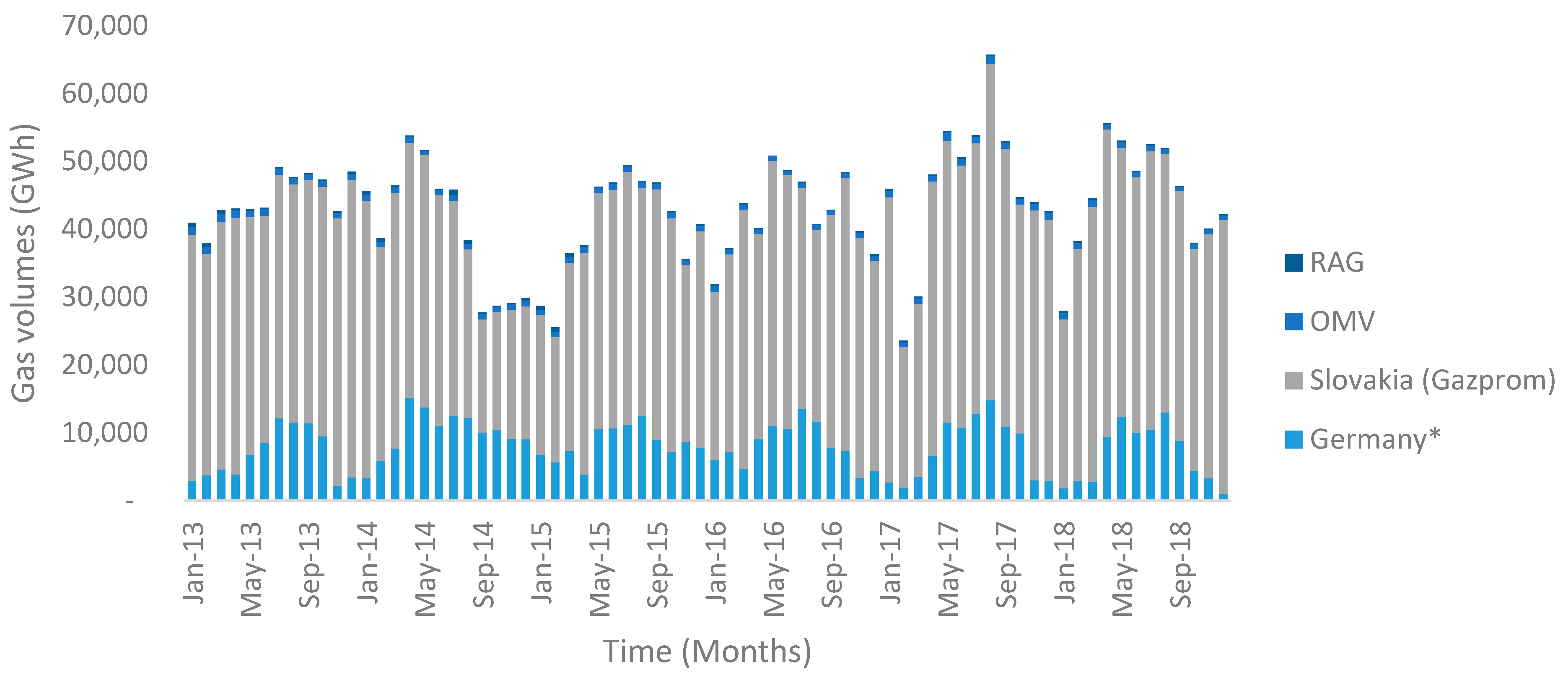
Austria imports more than two-thirds of its inland consumption. Most of the gas entering Austria is delivered from Russia through Gazprom, arriving at the key entry point Baumgarten. The remainder originates from Germany through the West-Austria-Gasleitung (WAG) pipeline, the physical connection at the border with Germany. The indigenous production is undertaken by two companies, OMV and RAG.
In addition to local producers, as seen in Figure 1, the Austrian market is supplied from the east on the one hand, where a single company is the only supplier, and from Germany on the other hand, where several big gas suppliers are active.
2.1.3. The Netherlands
The Dutch gas company Gasunie is operating an entry-exit tariff system for the gas transmission network in the Netherlands, similarly to the Austrian market. The Title Transfer Facility (TTF) is the virtual point where operating traders exchange gas titles in the Netherlands.
Gas is exported and imported by means of connections that are located near the borders to Germany and Belgium. Gas is also imported from the United Kingdom via Belgium through the bi-directional interconnector. Nonetheless, gas can only be directly imported via the connection with Norway in Emden, northern Germany.
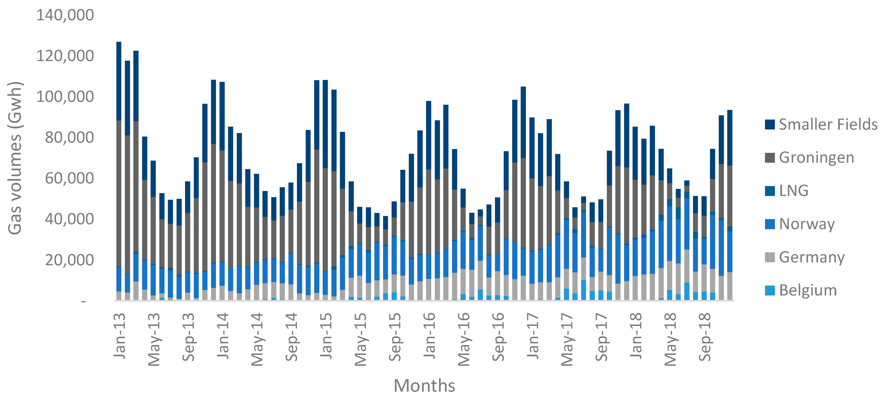
Gas consumed in the Netherlands mainly comes from local production, specifically the Groningen field, in addition to further onshore and offshore Dutch fields. The Netherlands is the principal gas producer in the EU.
Additionally, as per Figure 2, other sources feed the local market, such as imports from Russia, Norway, and LNG. More than two thirds of the total gas produced within the country originates from the Groningen field (Giant and biggest European gas field located in Netherland) and other onshore fields. The remainder is produced in 150 fields located offshore in the North Sea [30].
2.1.4. Key Performance Indicators of Both Gas Hubs
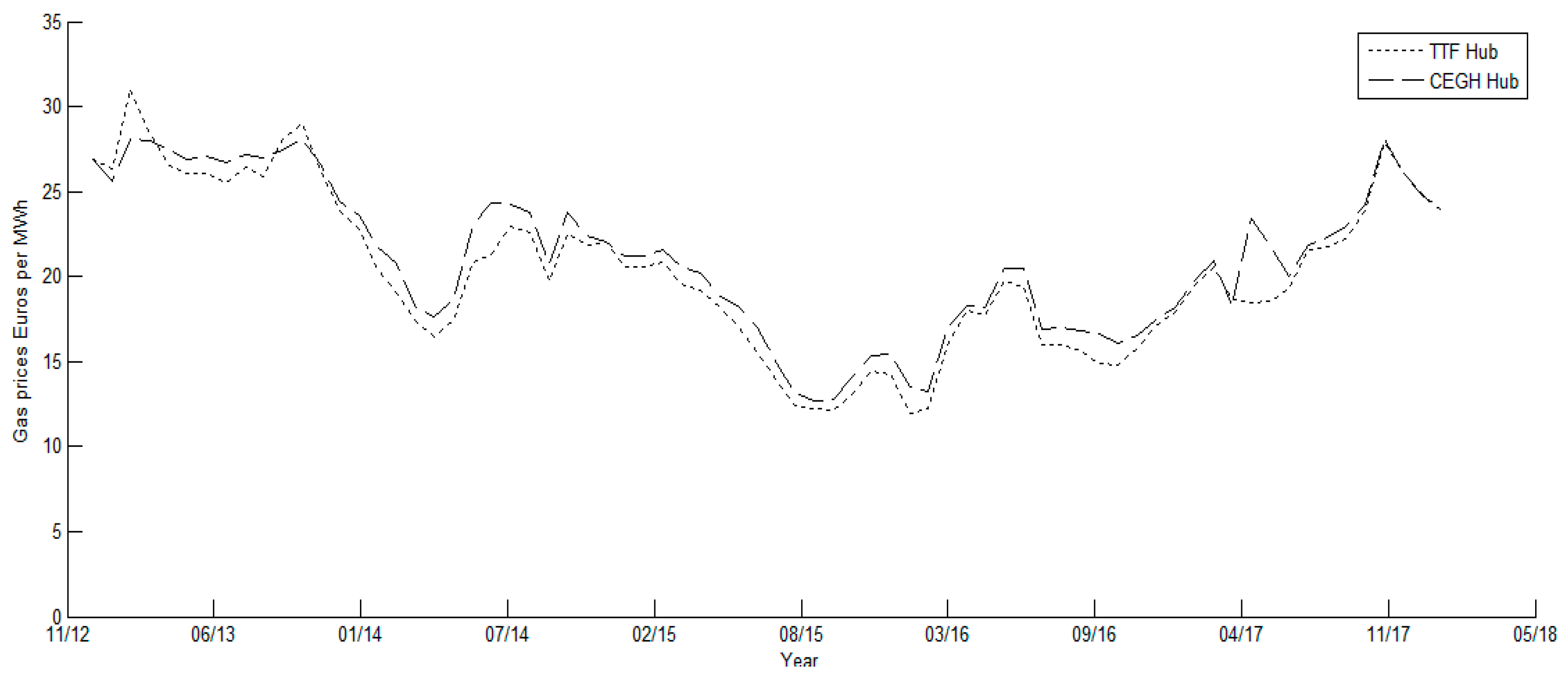
Another set of data that is important for this study is the wholesale gas price in each market. Figure 3 shows the time series of the natural gas prices of both the Dutch market, represented by the TTF hub, and the Austrian market, represented by the CEGH. All prices are denominated in Euros per MWh. The dataset consists of monthly values recorded between January 2013 and December 2018. As shown in the graph, both price trends are, to some extent, positively correlated, albeit the price of gas sold on the Austrian side is at most times higher than that on the Dutch market.
This price and volume behavior should usually be justified and interpreted by a solid understanding of the economics of both market structures and evaluated by means of a quantitative analysis, which is the subject of this research.
Some reports presented by think tanks such as [31,32,33] conducted an analytical analysis that can also provide an insight into market structure and prior formation of these gas markets. The results of these analytical studies are summarized below:
The number of firms trading at a hub indicates the willingness of traders to be involved and the ease of participation; a larger number of active participants is a sign of increased competition and consequently less market manipulation.
According to Table 1, the low quantity of gas traded in the CEGH is an indication of low liquidity in Austria, as compared with the Netherlands. On the other hand, Table 2 shows the churn rate, which is the traded volume as compared with the size of the market. It clearly highlights the fact that the Dutch market scores a high churn ratio, which is attractive for traders and financial players. However, this is not the case for the CEGH; the low churn rate and the low quantities of traded volumes indicate lower liquidity in Austria, an unattractive environment for traders and financial players. The churn ratio is a main factor in determining the success of a trading platform according to [10].
Based on the presented numbers, it can be directly concluded that the Dutch TTF hub is dynamic and less concentrated because of the liquidity and wide range of participants in the gas trade, unlike the CEGH in Austria.
These studies show the positive impact of the liberalization process on the gas price mechanism in Europe. More specifically, the northwestern part of Europe now reflects gas market supply and demand fundamentals. However, this is not yet fully the case in Central Europe, i.e., the CEGH. In other words, the gas-on-gas competition in Central Europe has increased from zero in 2005 (this means that prior to 2005, the contracts in the eastern part of Europe were wholly governed by long term contracts indexed on oil) to over 56% in 2015, with changes accelerating from 2013 onwards [32]. The gas indexation level in the TTF has reached higher norms.
By 2013, most of the Dutch and Norwegian long-term contracts had moved to hub prices. In fact, companies like Statoil, Gasterra, and UK producers shifted their gas contracts to hub indexation. Moreover, Russia and some of its customers agreed to revise the pricing formula by reducing the base price by about 10% and by reducing the take or pay commitment from as high as 90% to 60%. The only supply source that is still resistant to change is located in Algeria, where the gas supply contracts are still indexed on oil. Gazprom, Sonatrach, other key producers and several LNG exporting companies prefer long-term bilateral contracting with a higher presence of oil-price indexation [34].
As stated previously, the new regime foresees that any gas transported through the Austrian and Dutch networks is traded at the VTP where both bilateral and exchange trades are possible. Therefore, the large suppliers will sell their gas at both trading hubs. This means that both markets are interdependent, and that game theory is indeed a convenient model to analyze the strategic behavior of such companies. The following section elaborates on and presents the methods used in this analysis.
2.2. Non-Parametric Method
Translated into modeling, a country importing gas from different suppliers and the number of available observations is considered. For each and , the gas price at period is denoted by and the quantity of gas supplied by supplier at period t by . The monthly data related to supply and prices are illustrated in Figure 1, Figure 2 and Figure 3.
The classical Cournot equilibrium test, which is designated as the parametric method in this study, takes into account several assumptions on cost and demand functions and yields an optimization problem. The simplest way to solve such an optimization problem is by applying the Krush-Kuhn-Tucker (KKT) principle to solve the following objective function
where the first derivative of the inverse demand function is , is the marginal cost of the gas, and where the total quantity supplied to the relevant markets is,
The latter objective function is the profit maximization strategy of each gas supplier, and the success of solving this problem is not constrained by mathematical theory. As long as there is a convex problem and the conditions of the KKT are satisfied, the optimal solution can be found. However, the problem lies in the assumptions of such empirical models. At the end of this section, the parametric method is further explained, and the different assumptions are enumerated.
As previously explained, a practical non-parametric theory to test if a data set with convex cost functions belongs to Cournot is developed. In the following paragraph, it is explained how this theory can be customized and applied to the natural gas market.
is defined as the marginal cost of supplier at period . The first-order condition of firm optimization problem previously defined in Equation (1) now states that there is contained in such that
The set of observations respects the Cournot equilibrium if both conditions mentioned below are met (these conditions are derived from Equation (3):
- The observed price in each period should belong to the inverse demand function; it follows that the array must obey the following condition
- At each period, firm i′s quantity level maximizes its profit subject to the quantity of the competing firms. This property can be stated as the following inequality
At first, it is essential to know and compare the values of marginal costs for each firm at each time . In other words, if firm is producing a quantity that is higher than the quantity produced by firm , this simply tells us that the marginal cost of the latter firm should in theory be higher than the former.
Condition 2 is then applied to extend the analysis from several firm output at a specific time , to a whole range of firm outputs at different time intervals. It will then be possible to compare the marginal costs of different firms and at different times. So, if firm produces a quantity at time t, and then changes its strategic outcome to a lower level , Equation (5) tells us that must be lower than . The same logic is repeated for firm j. Finally, this will lead us to combine the results of both condition 1 and 2, and then order the marginal costs for each firm and at each time in increasing order. Once this is completed, we can then check if this order respects Equation (4).
Since the constraints of a specific inverse demand function and a specific cost function, both of which are defined in Section 3, are lifted, prices and volumes can be tested in an algorithm to verify whether or not each observation respects the Cournot equilibrium. This algorithm is based on the results of the previous statements. It starts with an assumption of the highest possible marginal cost (Upper bound) of firm at , which is equal to the price (this is typical in a fully competitive market, where the price of any commodity (i.e., gas in our case) should be equal to its delivery cost.), and verifies if conditions 1 and 2 are met at each change in marginal cost level.
The Cournot acceptance rate is then calculated, which is the ratio of cases where conditions 1 and 2 are met to the total number of observations. A higher ratio means that the firms are competing under the umbrella of the a Cournot competition, each trying to behave strategically and willing to maximize its profit, taking into account what it believes to be a strategic output of its rival
Finally, in order to check if the changes in the concentration of suppliers affect the movement of gas prices in each market, the correlation coefficient between the prices . and the concentration index (the Herfindahl–Hirschman Index is used to calculate the concentration in each market) in each market is solved as follows,
The results of the non-parametric model applied for the first time to natural gas markets are then compared with the results of the parametric models that are used extensively in the literature. In order to highlight the complexity of making parametric assumptions, a brief description of the parametric method and its assumptions is presented below.
2.3. Parametric Method
Firstly, with regard to the cost assumptions, the production cost function of each supplier, in addition to its transportation costs, in this study follows the form proposed by the following articles: [14,35]. Equation (7) gives the capacity utilization marginal cost function :
where is the maximum production capacity of each supplier. The parameters are adjusted for inflation in order to fit the purpose of the study. The production cost functions are assumed to be convex and monotonically increasing.
As shown in Figure 1, the Austrian market is supplied by three main parties (OMV and RAG are counted as one indigenous supplier, since both are assumed to have the same marginal cost function. In addition, the indigenous gas producers in Austria are assumed to be price takers and therefore cannot influence the market price of the gas).
The cost assumptions (Equation (7) for the gas are shown in Table 3.
Secondly, assumptions on the price demand function are made. To this end, the price and volume data are fitted to a classical linear price function, .
The assumption of a simple linear regression model results in a low correlation coefficient. The authors acknowledge that there are many other explicative variables affecting the gas price and that it is more accurate to estimate the demand function using econometric models of high complexity level (i.e., vector autoregressive analysis using several supply and demand variables, machine learning, etc.). Due to the limited set of available data points, the fact that modeling the price function exceeds the scope of this paper, and the fact that the use of the parametric method is only limited to comparison purposes, the assumption of a simple linear regression model is made for the demand function.
The results and the use of simple linear regression and the least square principle are assumed to be indifferent to the possibility of endogeneity and correlation with error terms in this particular context. The market inverse demand function is a linear function with ay downward slope. Additional assumptions, such as price elasticity of demand, are made in order to obtain more accurate numbers (the price elasticity of demand is assumed to be −0.2 for both markets, Austria and the Netherlands. This is an assumption, and different values that range between −0.1 to −0.8 are found in the literature for oil and gas markets [37,38].). The final step of the optimization is to solve the system of nonlinear equations and apply the KKT principle. The number of equations depends on the number of suppliers that are competing in each market.
3. Results and Discussion of Results
3.1. Non-Parametric Analysis
The average concentration indexes for all the data in both markets show signs of a low level of competition, and the values of both hubs indicate that the gas markets are concentrated to a certain extent. However, when comparing both values shown in Table 4, the CEGH scores 0.68 and is thus much larger than the TTF market, which sits at a value of 0.3. These numbers are a clear indication that the latter market is moderately less concentrated than the former.
This indicates that the Netherlands leads the process of gas market liberalization, while other central hubs that are constrained by limited supply are lagging. Typically, as shown in Figure 1, the production and imports in a country like Austria are dominated by a large, state-controlled company that has limited competition from other suppliers, which are active in Germany, a factor that gives rise to oligopolistic market behavior.
In order to test the significance of the correlation coefficient describing the relation between prices and concentration indexes in both markets, the classical Student test is performed. The results of the test are listed in Table 4.
The p-value in the Austrian market indicates that the correlation coefficient, which stands at a low value of 0.20, is not significant, which is the reason why there is no linear correlation between prices and the degree of market concentration.
By contrast, the correlation coefficient at the Dutch market is of higher value and significance, and stands at 0.67. The causation relation between the change in wholesale gas prices and the concentration of market shares in the Dutch market highlights the market power that oligopolistic traders have and can exercise at a given time by simply considering different strategic quantities. Additionally, it is worth mentioning that the short-term price dynamics are also affected by variables such as weather, storage, exchange rates, and supply disruptions.
The results suggest that there is no clear causality during the years of 2013–2018 in the Austrian market, in which the number of suppliers is limited. Each supplier’s market share is large enough for even a modest change in strategic quantity by one large supplier to have a noticeable effect on the market shares or incomes of competent rivals. As for the results of the non-parametric test shown in Table 5, they indicate the following:
- ❖
- The behavior of large gas suppliers in both markets can be explained by a Cournot model, in which suppliers follow rational economics and try to maximize their payoffs. This is justified as more than 50% of the observations respect the Cournot equilibrium, which means that the suppliers in that market are acting strategically to maximize their profits. This is in line with authors [16,17,18,19,20,21], as all of them agree on the fact that the Cournot competition is the most elastic representation of the current gas markets in Europe.
- ❖
- Interestingly, both markets generate similar results, which mean that the suppliers in both markets follow the same behavior even though the concentration index indicates a more concentrated market in Austria. As stated previously, the TTF is less concentrated than the CEGH. In theory, this means that the behavior of the gas suppliers in the former market should show signs of competition.
- ❖
- There may be a reason why the acceptance rate does not converge to higher values. It could be that suppliers have other strategies in mind, such as collusion (few researchers have studied the market power relation to prices in the presence of collusion. Most notable is [4], who concludes that (i) collusion behavior can induce price response asymmetry and (ii) markets with few suppliers are more likely to observe this type of price response), as in oil markets with OPEC or other strategies that are not “pure” profit maximizers. In the case of collusion, the solution is no longer a non-cooperative Nash equilibrium. This is in line with the findings of [17], who suggested that Gazprom is maximizing a ‘utility function’ relative to the choice of two variables/objectives, one related to profit and another not related to profit. Others such as [16] suggested that certain European gas players are either not fully Cournot players or that the new regulations and perhaps still ongoing old legacy contracts prevent them from exerting full market power.
This analysis allows for compelling interpretation of this paper’s proposition: although the CEGH is less dynamic due to its few suppliers, the game theory results for both markets are quite similar, which is a clear indication of market integration. This is in line with several other studies, namely [27,39]. In addition, the correlation of both hub prices is calculated and results in a value of 0.98; close to 1. The reasons for the lack of full market integration are briefly summarized below:
Firstly, there may be storage problems that cause prices to increase, compared to adjacent markets, thus resulting in a decrease in correlation (if the price differential between the two markets is less than the transportation fees, there is a risk of arbitrage, and the prices do not return to equilibrium). Secondly, there is a lack of transport capacity, which creates bottlenecks at times. Finally, the existence of contractual congestion and the concern about capacity hoarding are a main barrier to market integration. Eni, the Italian multinational oil and gas Company, has long-term contracts to use 85–95% of Transitgas and TAG capacity and 67% of TENP capacity. Transitgas and TENP are gas pipelines that link Italy to Switzerland, Belgium, and the Netherlands on the one hand, and TAG links Italy and Austria on the other hand. Eni did not free up any unused capacity to either Transitgas or TAG. For this reason, the Italian antitrust regulator has opened an investigation for abuse of dominance position.
The high degree of market integration across Europe and the presence of strong liquid hubs in the northwest of the continent are bound to reduce the risk of market manipulation in the eastern part of Europe, where the gas hubs are less liquid and have a limited number of suppliers.
It is evident that due to the weak integration between gas markets and the lack of effective pricing mechanisms, suppliers in such markets can greatly influence the gas prices while the markets are isolated from trading opportunities arising in nearby countries. This is true for the European Baltic states, where Gazprom uses its dominant position to charge unfair prices [40].
3.2. Parametric Anlaysis
As previously mentioned, the Austrian market is supplied by three main parties. Based on the assumptions listed in the previous section, the optimal yearly quantities of each supplier are obtained by empirically solving Equation (1) with the use of KKT conditions. The strategic quantities that give the maximum return for all three suppliers in the Austrian market in 2013 are computed and listed in Table 6.
As can be seen, the computed quantities differ from the actual values. According to the complementarity solution and based on the demand and cost assumptions, these values are the result of the strategies that resulted in the equilibrium solution of the different companies involved in the Austrian gas market.
It is important to note that the quantities are different when compared to the actual values. Our model shows that in order to reach a Nash equilibrium for competing suppliers, greater gas quantities have to be imported from Germany. The final strategic quantities for each supplier are then inserted into the inverse demand function computed using the regression technique in order to calculate the final wholesale price. These prices are shown in Table 7. The same analysis is performed for the Dutch market.
Actual yearly average prices for the same years are shown in Table 8 below:
The results presented in Table 7 are comparable to the actual values in Table 8. The Nash equilibrium for all suppliers can lead to a price that is slightly lower than the actual prices in a certain year and higher in another. It is not easy to interpret such results. On the one hand, the resulting prices are similar to the actual prices, which indicates that the authors’ model and assumptions are accurate to some extent. On the other hand, these prices are the result of strategic quantities that are optimized and that are not to be compared with actual values. The parametric method can indeed compute the optimal quantities of each supplier and subsequently the gas clearing prices. However, this requires assumptions regarding the market price, demand function, strategy of each supplier and the cost functions thereof. For this reason, the interpretation of the parametric results may be misleading and cannot be validated. However, this is not the case for the non-parametric method and results pioneered in this paper.
4. Conclusions
This paper presents a novel approach to testing if the liberalization of the gas industry has led to less concentrated European gas markets and studies the behavior of gas suppliers. The study of gas markets in itself is not new; previous analyses followed classical parametric optimization methods, which focus on the use of empirical data and market assumptions about cost and demand functions, for this purpose. By contrast, the method used in this study requires no parametric assumptions about demand and cost functions.
Using the non-parametric method, the authors assess the degree of concentration in two different European gas markets, Austria and the Netherlands, where each represents a different evolutionary stage in the process of wholesale gas market liberalization.
The results show that the gas suppliers’ behavior in both the Dutch and Austrian markets follows the Nash–Cournot equilibrium and that they are rationally acting to maximize their payoffs. More importantly, it validates the fact the suppliers in both markets engage in the same conduct even though one market is more liquid than the other. The results also show that not all the observations respect the Cournot equilibrium, which means that the suppliers in that market are maximizing their ‘utility function’, not only by seeking profit but also by pursuing non-profit objectives, such as cooperative collusive behavior. This means that some suppliers are cooperating and thus exhibiting non-competitive behavior. Such suppliers adjust their strategies in conjunction with an agreed-upon understanding with the competing suppliers at the expense of the welfare of gas consumers and possibly smaller suppliers. In this case, the rule and assumptions of a typical Nash–Cournot equilibrium are not satisfied, and consumer gas prices are closer to monopoly prices despite the presence of several suppliers. A typical example of such a market and behavior is the presence of cartels in commodity markets.
Through non-parametric methods, an additional method for testing if European gas markets are integrated and if price convergence in the gas markets/hubs has really occurred over the years is provided.
Overall, the results presented in this study lead to the conclusion that the institutional changes do not deliver on the objective of increasing competition among suppliers directly in a given hub (i.e., do not have the power to influence the number of competitors). It is more beneficial to concentrate on enhancing market integration, thus improving access to gas from the lowest-cost gas sources. Accordingly, the risk of price manipulation is reduced by ensuring that the different gas hubs in Europe are highly integrated.
The gas market in the Dutch TTF is anticipating an important decision on the speed of further reduction in domestic production amid uncertainties about the Groningen field production rates, which is the main provider of gas to customers located in Northwestern Europe. The security of supply is again at stake, a factor that increases Europe’s dependence on gas imports [41]. Therefore, diversification of supply and market integration is of primary importance in Europe.
Antitrust regulators rely on further research and analyses of other suppliers’ behavior, such as collusion, in their quest to ban abusive behavior and in supervising mergers and acquisitions in both wholesale and retail markets. The role of the regulator is noteworthy, especially with regard to the method of non-parametric Cournot theory. The modeler can check if the strategies adopted by a supplier/company in a one- or few-stage game can be sustained or if it will lead to a different outcome. Future research may focus on updating and enhancing the parameters used in this study, mainly with regard to the cost functions of the relevant big gas suppliers.
Author Contributions
Conceptualization, H.H.; methodology, H.H.; formal analysis, H.H. and A.H.; software, H.H. and A.H.; project administration, H.A.; writing—original draft, H.H.; writing—review and editing, H.A. and H.H. All authors have read and agreed to the published version of the manuscript.
Funding
This research received no external funding.
Institutional Review Board Statement
Not applicable.
Informed Consent Statement
Not applicable.
Data Availability Statement
The data presented in this study are available on request from the corresponding author.
Conflicts of Interest
The authors declare no conflict of interest.
References
- Stern, J. International gas pricing in Europe and Asia: A crisis of fundamentals. Energy Policy 2014, 64, 43–48. [Google Scholar] [CrossRef]
- Mu, X. Weather, storage, and natural gas price dynamics: Fundamentals and volatility. Energy Econ. 2007, 29, 46–63. [Google Scholar] [CrossRef] [Green Version]
- Hamie, H.; Hoayek, A.; Kamel, M.; Auer, H. Northwestern European wholesale natural gas prices: Comparison of several parametric and non-parametric forecasting methods. Int. J. Glob. Energy Issues 2020, 42, 259–284. [Google Scholar] [CrossRef]
- Hong, W.H.; Lee, D. Asymmetric pricing dynamics with market power: Investigating island data of the retail gasoline market. Empir. Econ. 2018. [Google Scholar] [CrossRef]
- Nick, S.; Thoenes, S. What drives natural gas prices? A structural VAR approach. Energy Econ. 2014, 45, 517–527. [Google Scholar] [CrossRef] [Green Version]
- Misund, B.; Oglend, A. Supply and demand determinants of natural gas price volatility in the U.K.: A vector autoregression approach. Energy 2016, 111, 178–189. [Google Scholar] [CrossRef] [Green Version]
- Čeperić, E.; Žiković, S.; Čeperić, V. Short-term forecasting of natural gas prices using machine learning and feature selection algorithms. Energy 2017, 140, 893–900. [Google Scholar] [CrossRef]
- Busse, S.; Helmholz, P.; Weinmann, M. Forecasting day ahead spot price movements of natural gas An analysis of potential influence factors on basis of a NARX neural network. In Multikonferenz Wirtschaftsinformatik 2012 Tagungsband der MKWI 2012; Institut für Wirtschaftsinformatik: Braunschweig, Germany, 2012. [Google Scholar]
- Hamie, H.; Hoayek, A.; Auer, H. Modeling the price dynamics of three different gas markets-records theory. Energy Strategy Rev. 2018, 21, 121–129. [Google Scholar] [CrossRef]
- Robinson, T. Have European gas prices converged? Energy Policy 2007, 35, 2347–2351. [Google Scholar] [CrossRef]
- Neumann, A.; Cullmann, A. What’s the story with natural gas markets in Europe? Empirical evidence from spot trade data. In Proceedings of the 9th International Conference on the European Energy Market, EEM, Florence, Italy, 10–12 May 2012. [Google Scholar]
- Hulshof, D.; van der Maat, J.P.; Mulder, M. Market fundamentals, competition and natural-gas prices. Energy Policy 2016, 94, 480–491. [Google Scholar] [CrossRef] [Green Version]
- Asche, F.; Misund, B.; Sikveland, M. The relationship between spot and contract gas prices in Europe. Energy Econ. 2013, 38, 212–217. [Google Scholar] [CrossRef]
- Golombek, R.; Gjelsvik, E.; Rosendahl, K.E. Effects of liberalizing the natural gas markets in Western Europe. Energy J. 1995, 16, 85–111. [Google Scholar] [CrossRef]
- Aune, F.R.; Golombek, R.; Kittelsen, S.A.C.; Rosendahl, K.E. Liberalizing the energy markets of Western Europe A computable equilibrium model approach. Appl. Econ. 2004, 36, 2137–2149. [Google Scholar] [CrossRef]
- Egging, R.; Gabriel, S.A.; Holz, F.; Zhuang, J. A complementarity model for the European natural gas market. Energy Policy 2008, 36, 2385–2414. [Google Scholar] [CrossRef] [Green Version]
- Jansen, T.; van Lier, A.; van Witteloostuijn, A.; von Ochssée, T.B. A modified Cournot model of the natural gas market in the European Union: Mixed-motives delegation in a politicized environment. Energy Policy 2012, 41, 280–285. [Google Scholar] [CrossRef]
- Egging, R.G.; Gabriel, S.A. Examining market power in the European natural gas market. Energy Policy 2006, 34, 2762–2778. [Google Scholar] [CrossRef]
- Gabriel, S.A.; Kiet, S.; Zhuang, J. A Mixed Complementarity-Based Equilibrium Model of Natural Gas Markets. Oper. Res. 2005, 53, 799–818. [Google Scholar] [CrossRef]
- Gabriel, S.A.; Zhuang, J.; Kiet, S. A large-scale linear complementarity model of the North American natural gas market. Energy Econ. 2005, 27, 639–665. [Google Scholar] [CrossRef]
- Holz, F.; von Hirschhausen, C.; Kemfert, C. A strategic model of European gas supply (GASMOD). Energy Econ. 2008, 30, 766–788. [Google Scholar] [CrossRef] [Green Version]
- Massol, O.; Banal-Estañol, A. Market power and spatial arbitrage between interconnected gas hubs. Energy J. 2018, 39, 67–95. [Google Scholar] [CrossRef]
- Forges, F.; Minelli, E. Afriat’s theorem for general budget sets. J. Econ. Theory 2009, 144, 135–145. [Google Scholar] [CrossRef] [Green Version]
- Ray, I.; Zhou, L. Game theory via revealed preferences. Games Econ. Behav. 2001, 37, 415–424. [Google Scholar] [CrossRef] [Green Version]
- Sprumont, Y. On the Testable Implications of Collective Choice Theories. J. Econ. Theory 2000, 93, 205–232. [Google Scholar] [CrossRef]
- Carvajal, A.; Deb, R.; Fenske, J.; Quah, J. Revealed Preference Tests of the Cournot Model. Econometrica 2013, 81, 2351–2379. [Google Scholar] [CrossRef]
- Kuper, G.H.; Mulder, M. Cross-border constraints, institutional changes and integration of the Dutch-German gas market. Energy Econ. 2016, 53, 182–192. [Google Scholar] [CrossRef] [Green Version]
- Kema, D. Country Factsheets. 2013. Available online: https://ec.europa.eu/energy/sites/ener/files/documents/201307-entry-exit-regimes-in-gas-parta-appendix.pdf (accessed on 23 November 2020).
- Thomas, S. Gas Regulation. Geeting thre Deal Through. 2018. Available online: https://gettingthedealthrough.com/area/15/jurisdiction/25/gas-regulation-austria/ (accessed on 23 November 2020).
- Anouk, H. The Dutch Gas Market: Trials, Tribulations and Trends. 2017. Available online: https://www.oxfordenergy.org/publications/dutch-gas-market-trials-tribulations-trends/ (accessed on 23 November 2020).
- Petrovich, B. The Cost of Price De-Linkages between European Gas Hubs; The Oxford Institute for Energy Studies: Oxford, UK, 2015; Volume 101. [Google Scholar]
- Heather, P. European Traded Gas Hubs: An Updated Analysis on Liquidity, Maturity and Barriers to Market Integration; The Oxford Institute for Energy Studies: Oxford, UK, 2017. [Google Scholar]
- Heather, P. The Evolution of European Traded Gas Hubs; The oxford institute for Energy Studies: Oxford, UK, 2015; Volume 104. [Google Scholar]
- ACER. Annual Report on the Results of Monitoring the Internal Gas Markets in 2016. 2017. Available online: https://acer.europa.eu/Official_documents/Acts_of_the_Agency/Publication/ACER%20Market%20Monitoring%20Report%202016%20-%20GAS.pdf (accessed on 23 November 2020).
- Golombek, R.; Gjelsvik, E.; Rosendahl, K.E. Increased competition on the supply side of the western European natural gas market. Energy J. 1998, 19, 1–18. [Google Scholar] [CrossRef]
- Blitzer, C. Western European Natural Gas Trade Model; MIT International Gas Trade Project; Center for EnergyPolicy Research, MIT Energy Laboratory: Cambridge, MA, USA, 1986. [Google Scholar]
- Huppmann, D. Endogenous Shifts in OPEC Market Power—A Stackelberg Oligopoly with Fringe; DIW Berlin: Berlin, Germany, 2014. [Google Scholar]
- Hamilton, J.D. Understanding crude oil prices. Energy J. 2009, 30, 179–206. [Google Scholar] [CrossRef] [Green Version]
- Capece, G. The Evolution of the Natural Gas Supply in Italy: From the Virtual Trading Point to the Gas Exchange. Procedia Soc. Behav. Sci. 2014, 109, 210–214. [Google Scholar] [CrossRef] [Green Version]
- European Commission. Antitrust: Commission Sends Statement of Objections to Gazprom for Alleged Abuse of Dominance on Central and Eastern European Gas Supply Markets. 2015. Available online: https://ec.europa.eu/commission/presscorner/detail/en/IP_15_4828 (accessed on 23 November 2020).
- Wook-Mackenzie. Shell and ExxonMonil’s Groningen Future Lies on Shaky Ground. 2018. Available online: https://www.google.com.hk/url?sa=t&rct=j&q=&esrc=s&source=web&cd=&cad=rja&uact=8&ved=2ahUKEwjbyMiP4e_tAhU9y4sBHZs-CvgQFjAAegQIBBAC&url=https%3A%2F%2Fwww.woodmac.com%2Freports%2Fupstream-oil-and-gas-shell-and-exxonmobils-groningen-future-lies-on-shaky-ground-15497&usg=AOvVaw1GoOKkAYoQSexvrWpMduzw (accessed on 23 November 2020).
Figure 1.
Monthly gas imports to Austria and indigenous production. Source: E-Control. The data related to the imports of gas to Austria and for the indigenous production by OMV and RAG are provided by E-Control and AGGM Austria (https://www.e-control.at/en/ and https://www.aggm.at/en). * Additional suppliers active in the market Area East receive gas from several gas shippers that are active in Germany.

Figure 2.
Monthly gas import volumes to the Netherlands and indigenous production. Source: Gasunie. The data related to the import of gas to the Dutch market can be found on the Gasunie website (https://www.gasunietransportservices.nl/en/).
Figure 2.
Monthly gas import volumes to the Netherlands and indigenous production. Source: Gasunie. The data related to the import of gas to the Dutch market can be found on the Gasunie website (https://www.gasunietransportservices.nl/en/).

Figure 3.
Monthly gas prices for the two gas hubs, Euros/MWh (available upon request for research students from market and information services at the European Energy Exchange, [email protected].).
Figure 3.
Monthly gas prices for the two gas hubs, Euros/MWh (available upon request for research students from market and information services at the European Energy Exchange, [email protected].).


Table 1.
Virtual Trading Point (VTP) participation.
| Hub | Market Participants | Active Participants | Total Traded Volumes (Twh) | |||||
|---|---|---|---|---|---|---|---|---|
| 2011 | 2014 | 2011 | 2014 | 2018 | 2014 | 2015 | 2018 | |
| TTF | 60 | 130 | 45 | 45 | 167 | 13,555 | 17,080 | 40,390 |
| CEGH | 40 | 53 | 15 | 15 | 72 | 400 | 340 | 970 |
Table 2.
Churn rate.
| Hub | Churn Rate [%] | ||||
|---|---|---|---|---|---|
| 2011 | 2014 | 2015 | 2017 | 2018 | |
| TTF | 13.9 | 36 | 45.9 | 54.3 | 70.9 |
| CEGH | 2.2 | 4.8 | 3.9 | 5.3 | 6.9 |
Table 3.
Cost assumptions parameters.
| Gas Origin | Gas Yearly Prices (USD Per Toe) 1 | |||
|---|---|---|---|---|
| Gas from Russia (Gazprom) | 22 | 0 | −41 | 100 |
| Gas from Norway/UK | 69 | 1 | −18 | 80 |
| Gas from the Netherlands (Indigenous) | 5 | 0 | −22 | 70 |
1 For the cost of production data and the value of the parameters included in Table 3, please refer to the studies of [14,35,36], more specifically the sections related to the cost of production. The cost of the gas from the German market NCG (NetConnect Germany) hub to Austria is computed based on an average of gas coming from all three directions (Russia, Norway and the Netherlands).
Table 4.
Correlation coefficient and significance.
| Hub | Concentration Index | Correlation Coefficient | p-Value |
|---|---|---|---|
| CEGH | 0.68 | 0.20 | 0.14 |
| TTF | 0.30 | 0.67 | 0 |
Table 5.
Cournot acceptance rate.
| Gas Hub | Cournot Acceptance Rate [%] |
|---|---|
| CEGH | 56 |
| TTF | 49 |
Table 6.
Strategic output of each supplier—Austria, 2013.
| 2013 | Outputs of Each Supplier-Austria | |
|---|---|---|
| Computed Quantities GWh | Actual Values GWh | |
| Russia (Gazprom) | 17,104 | 36,531 |
| Germany | 16,715 | 6728 |
| Indigenous | 1264 | 1264 |
Table 7.
Parametric method—yearly gas price results (in USD per tons of oil equivalent).
| Hub | Gas Yearly Prices (USD Per Toe) | |||||
|---|---|---|---|---|---|---|
| 2013 | 2014 | 2015 | 2016 | 2017 | 2018 | |
| TTF | 343 | 251 | 254 | 174 | 222 | 307 |
| CEGH | 340 | 297 | 271 | 193 | 240 | 319 |
Table 8.
Actual values—yearly gas price results (in USD per tons of oil equivalent).
| Hub | Gas Yearly Prices (USD Per Toe) | |||||
|---|---|---|---|---|---|---|
| 2013 | 2014 | 2015 | 2016 | 2017 | 2018 | |
| TTF | 348 | 268 | 253 | 179 | 227 | 305 |
| CEGH | 348 | 285 | 264 | 190 | 238 | 317 |
Publisher’s Note: MDPI stays neutral with regard to jurisdictional claims in published maps and institutional affiliations. |
© 2020 by the authors. Licensee MDPI, Basel, Switzerland. This article is an open access article distributed under the terms and conditions of the Creative Commons Attribution (CC BY) license (http://creativecommons.org/licenses/by/4.0/).
Share and Cite
MDPI and ACS Style
Hamie, H.; Hoayek, A.; Auer, H. Modeling Post-Liberalized European Gas Market Concentration—A Game Theory Perspective. Forecasting 2021, 3, 1-16. https://doi.org/10.3390/forecast3010001
AMA Style
Hamie H, Hoayek A, Auer H. Modeling Post-Liberalized European Gas Market Concentration—A Game Theory Perspective. Forecasting. 2021; 3(1):1-16. https://doi.org/10.3390/forecast3010001
Chicago/Turabian StyleHamie, Hassan, Anis Hoayek, and Hans Auer. 2021. "Modeling Post-Liberalized European Gas Market Concentration—A Game Theory Perspective" Forecasting 3, no. 1: 1-16. https://doi.org/10.3390/forecast3010001