Intracranial Pressure Forecasting in Children Using Dynamic Averaging of Time Series Data
by
Akram Farhadi
1,*, 
Joshua J. Chern
2,†,
Daniel Hirsh
2,†,
Tod Davis
3,†,
Mingyoung Jo
2,†,
Frederick Maier
4,† and
Khaled Rasheed
1,4,† 1
Department of Computer Science, University of Georgia, Athens, GA 30602, USA
2
Children’s Healthcare of Atlanta, Atlanta, GA 30329, USA
3
Cedars-Sinai Medical Center, Los Angeles, CA 90048, USA
4
Institute for Artificial Intelligence, University of Georgia, Athens, GA 30602, USA
*
Author to whom correspondence should be addressed.
†
These authors contributed equally to this work.
Forecasting 2019, 1(1), 47-58; https://doi.org/10.3390/forecast1010004
Submission received: 17 June 2018
/
Revised: 17 July 2018
/
Accepted: 31 July 2018
/
Published: 6 August 2018
Abstract
:Increased Intracranial Pressure (ICP) is a serious and often life-threatening condition. If the increased pressure pushes on critical brain structures and blood vessels, it can lead to serious permanent problems or even death. In this study, we propose a novel regression model to forecast ICP episodes in children, 30 min in advance, by using the dynamic characteristics of continuous intracranial pressure, vitals and medications during the last two hours. The correlation between physiological parameters, including blood pressure, respiratory rate, heart rate and the ICP, is analyzed. Linear regression, Lasso regression, support vector machine and random forest algorithms are used to forecast the next 30 min of the recorded ICP. Finally, dynamic features are created based on vitals, medications and the ICP. The weak correlation between blood pressure and the ICP (0.2) is reported. The Root-Mean-Square Error (RMSE) of the random forest model decreased from 1.6 to 0.89% by using the given medication variables in the last two hours. The random forest regression gave an accurate model for the ICP forecast with 0.99 correlation between the forecast and experimental values.
1. Introduction
Skulls are fixed volume vaults containing the brain, blood and Cerebrospinal Fluid (CSF). The brain tissue occupies about 80% of the total intracranial volume. The remaining contains about 10% blood in arteries and veins and about 10% CSF in the ventricles, the basal cisterns and the subarachnoid space [1]. The total volumes are constant, and an increase in one should offset by an equal decrease in the other. Otherwise, the pressure increases. Intracranial Pressure (ICP) is normally measured by assuming that it is evenly distributed among all intracranial compartments, including the intradural space of the spinal canal [2,3]. The normal ICP in healthy children is usually considered in the range of 5 to 15 mmHg.
Various pathological conditions may result in an increase in the ICP. In Traumatic Brain Injury (TBI), an ICP increase of >20 mmHg for more than 5 min is widely accepted to be detrimental [4]. The main purpose of ICP monitoring in TBI is to prevent secondary injury resulting from an increase in the ICP. In addition, measuring the ICP and Mean Arterial Pressure (MAP) allows calculation of Cerebral Perfusion Pressure (CPP): CPP = MAP − ICP [5]. Attempts can then be made to optimize the CPP with the goal of preventing cerebral ischemia.
The ICP is commonly measured using fiber-optics technology, which allows continuous ICP monitoring without CSF drainage. The fiber-optic type of catheter can be placed in the subdural space or the brain parenchyma [6,7]. In this study, we create a forecasting model using the data that were collected in a minute-based cycle in the pediatric intensive care unit. Our time series data cover the period of 2013 to 2017.
Despite the importance of the continuous measurement of the ICP, signal processing capabilities in existing commercial ICP monitoring devices remain poor, providing clinicians with less information that is confined to the mean ICP. Accordingly, clinical decisions related to treating abnormalities of the ICP are typically made solely based on the mean ICP, although raw continuous waveform data are usually available [8,9]. Mathematical models that relate the ICP dynamics to the other physiological parameters, the monitoring of which is minimally invasive, provide a powerful alternative for the patients who might benefit from a direct measurement of the ICP.
Ursino et al. [10] used a model to forecast the ICP dynamics from non-invasive measurements of arterial blood pressure, which appeared to conform to the ICP measured in the patients with Traumatic Brain Injury (TBI) [11]. Guiza [12] developed a model to forecast the increase in ICP in 264 brain-injured patients 30 min in advance using dynamic information of four hours ahead with 0.72 accuracy. They forecasted the increase in ICP as high or low rather than the actual value of ICP that we forecasted in this study using regression.
The eventual goal of this study is to use data-driven models that enable accurate ICP forecasts in real time. After preprocessing the data, a forecasting model is created to forecast the next 30 min of the ICP. Multiple regression algorithms are evaluated, and finally, a random model is selected to forecast the outcomes’ reliability.
2. Methods
The Institutional Review Board (IRB) of the Children Health Care of Atlanta (CHOA) approved to review 78 subjects’ charts between 9 January 2013 and 2 January 2017. An overview of the collected data is reported in Table 1 in the Results Section.
2.1. Data Acquisition and Preprocessing
We used the vitals, ICP and medications data for children at Egleston and Scottish Rite hospitals from September 2013 to February 2017. The data were stored in Hadoop [13], and the monitored ICP data were consecutively added to the database. In 1996, the Health Insurance Portability and Accountability Act (HIPAA) suggested some general requirements to enforce the security of protected health information [14]. After getting approval from HIPPA, we extracted Intensive Care Unit (ICU) patients’ raw data using database queries.
We monitored 78 patients’ ICP using the Integra Camino system. All transducers were implanted in the brain parenchyma. Given the diversity of children’s ages, we used “year” as their age unit. The length of ICP monitoring was considered to be per “day”, both because of the short-term ICP monitoring for some patients and the small median of patients’ ICP monitoring (less than a month). Time-averaged values of ICP, MAP and CPP were recorded per minute by the Phillips medical system in Atlanta, GA. The vitals include Heart Rate (HR), Respiratory Rate (RR), Blood Pressure (BP) and MAP. Missing data were possibly due to monitoring disconnections or data loss during patient transportation. Dealing with the missing data in the dataset is a frequent problem, and it may affect the final forecasting model significantly. To solve this issue, we impute the missing values if they were missing by less than 50% in the dataset. There are different methods for imputing missing values, which are based on other available data. Due to the long time needed for multivariate imputation, we decided to use simple mean imputation where the missing observation of a variable is replaced by the mean of the non-missing observations. Otherwise, if data were missing by more than 50%, we removed that feature [15,16]. These features were medications that were given to the patients.
2.2. Statistical Analysis and Machine Learning
The simple Pearson correlation method was used to see if there was any meaningful correlation between ICP and the changes in vitals during the patients’ ICP monitoring at the hospital.
We split the 78 patients into 52 and 26 individuals in two groups of training and testing, randomly. The median of the length of ICP monitoring for the patients was 17 days. In the training group, the length of ICP recordings (days) for 38 patients was less than 17 days. In the testing group, 16 patients had a length of ICP recording less of than 17 days.
We used Autoregressive Integrated Moving Average (ARIMA) and Exponential Smoothing (ETS) models to forecast ICP. The ARIMA model analyzes and forecasts uniformly statistic information, transmission and intercession of data [17]. This model is well specified when the underlying process is linear. The ETS model, as a robust stochastic model, does not only rely on the correlation of data. In this approach, the most recent observations were weighted higher than the previous ones. Therefore, the ETS model can produce smarter forecasts compared to the average method [18,19]. In order to forecast the next 30 min of a patient ICP, both the ARIMA and ETS models were fitted to the ICP time series data. Within an ARIMA model, there are three variables; auto-regressive (p), differencing (d) and moving average (q), and the model is often notated as (p,d,q). These parameters were optimized using auto.arima() in R software (3.0.2). On the other hand, ETS (M,A,N) forecasts by multiplying errors (M), adding trends (A) and ignoring seasonal effects (N).
We also used dynamic averaging time series to forecast ICP (see Figure 1). The choices of delay time and embedding dimension are important; as good choices can reduce both the amount of required data and the effect of any noise. The optimum values of the embedding parameters were determined by sensitivity analyses. This analysis is concerned with the behavior of the optimal solution with respect to the parameters. Let us consider the time series of . Xconstructed by the sliding window and Y would be our input and output matrices, respectively. The sliding window with a fixed size of two hours was used to forecast the next thirty minutes. Since it may not be feasible to forecast all of next thirty minutes at once, only one step ahead of a five-minute forecast was produced each time.
Dynamic features were used for a two-hour prediction period, as shown in Figure 1.
Each data point is the mean of 5 min of data calculated by:
Based on the domain experts’ idea and literature review, the ICP change in less than five minutes is not considered to be dangerous, and averaging can help to smooth our data. The forecast horizon was one since the forecast was one step ahead. In the first row, the working window includes k historical observations , which were used to forecast the next value . In the second row, the oldest value was removed from the window, and the latest value was added, keeping the length of the sliding window constant at k. The next forecast value would be , and so on, until the end of the dataset. If the number of observations is N, then the total number of data points is . After creating this matrix, %66 of data were used for training and %33 were used for testing set and details, as tabulated in Table 1.
Dynamic features included MAP, CPP, BP, ICP, RR, HR and medications. Medications that were given in the last hour included morphine, mannitol, Versed, saline-3 pct, pentobarbital, Dilaudid, lorazepam, rocuronium, fentanyl, succinylcholine and vecuronium. Non-overlapping intervals per minute were selected to extract these features. Medications data were added to the feature set as binary values, considering whether they were consumed at those time intervals or not. The observations showed minute by minute feature changes for each patient. Linear regression, Lasso regression, support vector machine and random forest were implemented to forecast the next 30 min of the ICP using the dynamic feature sets.
Running a regression is a simple statistical way to establish a relationship between a dependent variable and a set of independent variable(s). The Lasso regression, which performs both variable selection and regularization, showed less error in forecasting using our data comparing to the linear-based regression model. This regression is based on the shrinkage estimation, and it is a popular tool for the analysis of a high-dimensional dataset such as ours. The advantages of Lasso include: (1) a smaller Mean Squared Error (MSE) compared to the conventional methods; (2) handling the multicollinearity problems more efficiently; (3) weighting the features reliably; and (4) shrinking coefficients [20,21,22].
The Support Vector Machines (SVM) technique, which is based on statistical learning theory [23], provided better results in forecasting compared to the other regression models we used for our study. It can be applied not only to classification, but also to the case of regression. Still, it contains all the main features that characterize the maximum margin. A regression function is generated by applying a set of high dimensional linear functions. Hence, given a set of data (where is the input vector is the actual value and N is the total number of data patterns), the regression function can be presented as: . In this equation, is the weighted vector, b is the constant and denotes a mapping function that is utilized in the feature space. The coefficients and b) are calculated by minimizing the regularized risk function as follows:
where:
In Equation (2), C and are user-defined parameters and is called an -insensitive loss function. The parameter is the difference between the actual values and the values calculated from the regression function. This difference can be treated as a tube around the regression function. The loss equals zero if the forecast value is within the -tube. Furthermore, is used to estimate the flatness of a function. Thus, C is a parameter determining the trade-off between the empirical risk and the model flatness. It corresponds to a linear method in a high dimensional nonlinear feature space related to the input space and carries out the regression estimation by risk minimization. This risk minimization consists of the empirical error and the confidence level value.
The SVM method might prevent the over-fitting problem since the feasible region is a convex set. This would make the SVM solution a global optimum [24]. Here, we used a polynomial kernel of degree one to represent the similarity of the training samples in a feature set over polynomials of the original variables.
We also used the random forest method [25] to build our prediction model. This model is made of many different decision trees generated from a random bootstrap decision sampling of the same training data. Decision trees can divide the feature space into a number (J) of regions and fit a specific model in each one. The decision model assigns a constant value, , to each region as: if then . Thus, a regression tree can be defined as:
where:
At each inner node during the regression process, the RF traverses down the data to choose the best splitting feature that results in the highest information gain from a small number of randomly-selected features rather than using all the features. Finally, the output is calculated as the arithmetic mean of all individual tree predictions [26]. The random forest has many of advantageous aspects that make it very suitable for many prediction problems. First, it is fast enough to apply on a regression problem; second, it is robust to the noise; and third, it handles a high number of features easily [27]. The random forest was chosen to handle the multicollinearity of the features as explained above.
3. Results
Overall, 78 patients with continuous ICP monitoring were chosen for this analysis. Out of these 78 patients, 42 were male and 36 were female. The number of children who were less than eight years old and more than eight years old was 44 and 34, respectively. According to the patient’s length of ICP recording, there were 54 recorded less than 17 days and 24 recorded for a longer time (Table 1).
Figure 2 shows the Pearson correlation among vitals and ICP. Pearson correlation [28] results demonstrated a lack of significant correlations between vitals and ICP.
There is a poor positive correlation between HR and RR. Other than that, there is not any meaningful correlation among vitals in Figure 2. In this study, we did not add any information regarding the types of traumatic brain injury including brain contusion, brain bleed and brain shift, a notable omission.
This study focused on evaluating the forecasting performances of various models for both the short and relatively long term. The sliding window w was set to be two hours of ICP data by minute, and the forecasting horizon k was set to five, meaning five forecasts were produced ranging from five minutes ahead to 30 min ahead into the future. After preprocessing, 66% of data were used for training and 33% of data for testing, considering the normal distribution among features in both sets.
A baseline, linear regression did the worst in forecasting time series as it was not able to predict the change points in the forecast line. Exponential time series did a better job than simple linear regression with lower error rates. ARIMA reduced the mean absolute error to around one, but kept the squared correlation coefficient the same as the two previous forecasting algorithms.
Figure 3 compares the ICP forecasting for a patient during the next 30 min using both of these models.
Both forecast estimates above were provided with confidence bounds: 80% confidence limits shaded in darker blue, and 95% in lighter blue. Longer term forecasts usually have more uncertainty, as the model regresses future Y on previously predicted values. As you can see, after a sharp change in ICP, neither ETS nor ARIMA can forecast accurate values of continuous ICP. We obtained an RMSE of 3.3 using ETS. ARIMA reduced this amount of error to 3.0. However, due to the non-stationary nature of some of the patients ICP data, we could not track the same pattern using ARIMA.
To create better prediction model, we used two hours of vitals and medication to create dynamic features based on a sliding window every five minutes. Two Lasso regression and random forest used for regression. Plots represented in Figure 4 and Figure 5 helped to choose the most accurate model to fit our data the best.
In Figure 4 each color represents the value taken by a different coefficient in the Lasso model. As it is shown here, with the small L1 norm, there was much regularization. On the other hand, as Lambda grew, the regularization term had a more substantial effect, and we saw fewer variables in our model (because more and more coefficients will be normed to zero). Lasso simultaneously selected relevant predictive variables and optimally estimated their effects [29].
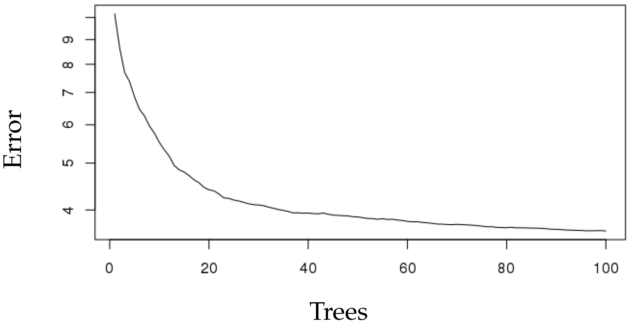
We also applied random forest for forecasting the next 30 min of ICP. Random forest increases diversity among the regression trees by resampling the data with replacement and randomly changing the predictive variable sets over the different tree induction processes. In current work, we used R software to build regression trees. For the training of this type of model, it is necessary not only to define the space dimensionality of random features, but also the number of trees to be built based on the decision limits generated by said division variables. To establish the optimal value of these parameters, a number of experiments were carried out using a different number of trees and a different number of split variables. The number of trees ranged between one and 100. Figure 5 shows our trained random forest tree performance with 100 trees and the related error.
As you can see, MSE decreased as the number of tree increased. Prediction accuracy of all algorithms was assessed using the squared correlation coefficient between predicted ICP and actual ICP values in the next 30 min, Mean Absolute Error (MAE), RMSE and Relative Root Squared Error (RRSE) (see Table 2).
RMSE for Lasso regression was 2.76. the RRSE changed from 31 to 21.5% after adding medications. In support vector machine, the error rate was less than linear regression. However, comparing to other regression results, random forest explained more of the variability of the response data around its mean. The algorithms used for prediction are listed in Table 2.
Lasso regression and support vector machine achieved the same ; however, the RRSE of support vector machine was significantly less than Lasso regression. Finally, the best model, random forest, obtained the least RRSE for the forecast. For the selection of the best regression model, we determined that it was the one in which the several error rates were lower than the other algorithms. From the numbers in Table 2, it is immediately obvious that random forest outperformed other algorithms in forecasting. Adding medications decreased RMSE from 1.6 to 0.89 using random forest. This helps the physicians to read predictions for the next 30 min using the last two hours of data. A squared correlation coefficient of 0.99 implied that the random forest model explained 99% of the variance in our data. Furthermore, this model resulted in a less average distance of predictions from actual data points (0.59).
4. Discussion
The clinical context of this research is using a novel approach to generate continuous, streaming next-30-min ICP forecasts to facilitate ICP management. Currently, intervention is implemented until ICP rises above a certain threshold (20 mm HO). One may envision that eventually, it may be desirable for clinicians to intervene based on predictions before the actual rise of ICP. The dynamic time series forecasts non-stationary phenomena much better than ordinary forecasting, so it can preserve both higher and low frequency components of the ICP changes. In general, it is capable of revealing a certain trend of the data, which is likely to be missed by conventional techniques of using constant features for prediction.
The normal intracranial pressure increases with age, as cranial bones will be more rigid and structures close with age. Figure 6 shows ICP change with age.
Comparing ICP in different age groups shows that a small increment in intracranial volume results in a notable change in ICP. The pressure increase is faster in children and slower in older adults. In the presence of any intracranial masses (tumors, cysts or hydrocephalus), the ICP can increase rapidly. This sharp increase can decrease the Cerebral Blood Flow (CBF) significantly and cause cerebral ischemia and death [30,31]. Reliable prognosis of ICP trends with long prediction horizons is required for clinical purposes; this may be regarded as the multistep prediction task. In the experiment described in this paper, multi-step prediction has been used. Each row in the sliding window matrix was used to predict the next k steps ahead, and this iteration was repeated k times to achieve thirty minutes of prediction.
There have been multiple studies that have tried to forecast ICP; however, they did not consider medication’s effect on ICP forecasting. Several studies have done classification rather than regression to forecast ICP [32,33]. In this study, we presented different models for forecasting ICP in children based on dynamic features. We demonstrated that increased ICP could be forecast using time-based ICP changes in the past. However, ARIMA and ETS models did not work well because of erratic fluctuations in ICP, so they could not forecast them accurately. Applying regression models allow us to forecast ICP accurately 30 min ahead.
Forecasting ICP for k time steps with less error rate can be regarded as a really satisfactory result, even in comparison with the results achieved in other areas of interest [34,35]. This is possible mainly due to recent advances in data pre-processing, like preparing the dynamic sliding window for short-term and long-term forecasting. Nevertheless, what is a satisfactory result from the mathematical point of view may be quite disappointing in practical applications. In particular, no method of mathematical forecasting, available to date, is able to predict irregular and/or incidental break points in the signal, if they had not been heralded in the historical course of the process; whereas, in fact, prediction of such changes in the ICP trend as early as possible would be most valuable to the neurosurgeon and nurses. Hence, we shifted our interest from the “simple” long-term forecasting of the ICP to k step forecasting using dynamic time series features. Our ultimate goal was to describe an error rate of different machine learning algorithms to forecast k steps ahead of ICP.
To the best of our knowledge, this is the first forecasting that considers medications other than vitals in order to forecast ICP. This presents an advantage of intervening before the patient needs surgery in the operating room [36]. Our novel approach predicts the ICP average in children in the next 30 min, giving physicians and nurses enough time to make an intervention and decrease it by using specific medications. Future studies are required to investigate the effect of static features on predicting intracranial pressure.
5. Limitations of the Study
Limitations of this study should be noted. To deal with real-world problems, we are often faced with missing values in the data due to monitoring malfunctions or human errors. Handling different types of missing data was the only important limitation of this study. First, we only used a dataset of patients who had a bolt as they had less missing values. We removed the other dataset including patients who had an extra-ventricular device or patients who had been monitored with both a bolt and an extra-ventricular device, respectively, due to the high percentage of missing values. Second, surgery features had a high volume of missing values. We eliminated those features in order to achieve realistic results.
Traditionally, the missing values are simply omitted. However, omitting those missing values may cause temporal discontinuity. In order to prevent that, missing values were imputed using mean imputation. We believe having a complete dataset without needing to fill out missing values will improve the error rate of forecast.
6. Conclusions and Future Works
This study aimed to evaluate the performance of the multiple regressors for forecasting the next 30 min of ICP in children. Compared to other regressors, the random forest performed well in the context of regression with dynamic features of time series. The specific objectives were to study the behavior of forecasting models with a low resolution of data, adding dynamic features of medications given in the ICP monitoring time and testing error rates in different models. The results of this research provide new insights into the performance of random forest in the context of forecasting dynamic time series. The random forest does not over fit because of the validation set that was used for testing, the law of large numbers and only two user-defined parameters to be set: the number of trees and the number of random split variables. The number of trees is directly proportional to the regressors’ error rate until reaching a state (100 trees) in which the generalization error converges adopting values lower than 1%. Once the error has converged, the number of random variables only alters the regressors error rate slightly.
The forecasting of ICP in the next 30 min based on dynamic features can give a reasonable estimate for ICP, which provides an appropriate time for intervening before serious problems occur. Given the inclusion criteria of the study, all patients had an ICP device of a parenchymal electrode (Camino bolt). Having complete data of patients with the bolt would be a significant help in generalizing the model and using it for forecasting ICP in any types of patients.
In terms of future work, There are several directions that can be pursued in order to improve upon this work. More types of ICP monitoring data can be used, including patients who have an extra ventricular device for monitoring ICP. Other dynamic features such as surgical features could be helpful in generalizing the model. Furthermore, using other imputation models for missing values such as median imputation, random forest imputation or expectation maximization techniques might give realistic values compared to the simple mean imputation that was used here. Additional forecasting models, such as neural networks, especially recurrent neural networks, should be included in order to create a more comprehensive evaluation of the forecasting technique for intracranial pressure in children.
Author Contributions
A.F. involved in Conceptualization, Data curation, Formal analysis, Investigation, Methodology, Software development, and Writing. K.R. contributed to the supervision. F.M. contributed to the methodology and the software. D.H. contributed to the resources. T.D. contributed to the resources and investigation. J.J.C. was involved in the Conceptualization, Funding acquisition, Investigation, Supervision, Validation and writing. M.J., F.M. and J.J.C. contributed to Validation, Writing—review & editing.
Funding
This research received no external funding.
Acknowledgments
We acknowledge great support from the Children Health Care of Atlanta IS&T staff and Academic Neurosurgical Unit registrars. Without their help, the collection of electronic data would have never been successful. We also thank the University of Georgia for providing help in advising this study.
Conflicts of Interest
All other authors report no conflicts of interest relevant to this article.
References
- Linn, K. Acute Pediatric Neurology. Eur. J. Paediatr. Neurol. 2014, 18, 828. [Google Scholar] [CrossRef]
- Sankhyan, N.; Raju, K.V.; Sharma, S.; Gulati, S. Management of raised intracranial pressure. Indian J. Pediatr. 2010, 77, 1409–1416. [Google Scholar] [CrossRef] [PubMed]
- Palmer, J. Management of raised intracranial pressure in children. Intensive Crit. Care Nurs. 2000, 16, 319–327. [Google Scholar] [CrossRef] [PubMed]
- Klose, M.; Juul, A.; Poulsgaard, L.; Kosteljanetz, M.; Brennum, J.; Feldt-Rasmussen, U. Prevalence and predictive factors of post-traumatic hypopituitarism. Clin. Endocrinol. 2007, 67, 193–201. [Google Scholar] [CrossRef] [PubMed]
- Chambers, I.R.; Jones, P.A.; Lo, T.M.; Forsyth, R.J.; Fulton, B.; Andrews, P.J.; Mendelow, A.D.; Minns, R.A. Critical thresholds of intracranial pressure and cerebral perfusion pressure related to age in paediatric head injury. J. Neurol. Neurosurg. Psychiatry 2006, 77, 234–240. [Google Scholar] [CrossRef] [PubMed] [Green Version]
- Riordan, M.; Chin, L. Intracranial Pressure Monitors. In Adjuncts for Care of the Surgical Patient, An Issue of Atlas of the Oral & Maxillofacial Surgery Clinics 23-2, E-Book; Elsevier: Amsterdam, The Netherlands, 2015. [Google Scholar]
- Adams, H.; Kolias, A.G.; Hutchinson, P.J. The role of surgical intervention in traumatic brain injury. Neurosurg. Clin. 2016, 27, 519–528. [Google Scholar] [CrossRef] [PubMed]
- Hu, X.; Xu, P.; Scalzo, F.; Vespa, P.; Bergsneider, M. Morphological clustering and analysis of continuous intracranial pressure. IEEE Trans. Biomed. Eng. 2009, 56, 696–705. [Google Scholar] [PubMed]
- Farhadi, A.; Lloyd, B.; Groat, D.; Mirkovic, J.; Cook, C.B.; Grando, A. iDECIDE: A Mobile Application for Pre-Meal Insulin Dosing Using an Evidence Based Equation to Account for Patient Preferences. In Proceedings of the AMIA, Washington, DC, USA, 14–18 November 2014. [Google Scholar]
- Ursino, M.; Lodi, C.A. A simple mathematical model of the interaction between intracranial pressure and cerebral hemodynamics. J. Appl. Physiol. 1997, 82, 1256–1269. [Google Scholar] [CrossRef] [PubMed]
- Evans, D.; Drapaca, C.; Cusumano, J. Dynamics and Bifurcations in Low-Dimensional Models of Intracranial Pressure. In Mathematical and Computational Approaches in Advancing Modern Science and Engineering; Springer: Berlin, Germany, 2016; pp. 223–232. [Google Scholar]
- Güiza, F.; Depreitere, B.; Piper, I.; Van den Berghe, G.; Meyfroidt, G. Novel methods to predict increased intracranial pressure during intensive care and long-term neurologic outcome after traumatic brain injury: Development and validation in a multicenter dataset. Crit. Care Med. 2013, 41, 554–564. [Google Scholar] [CrossRef] [PubMed]
- Stonebraker, M. Is MR a DBMS? MIT Computer Science and AI Lab: Cambridge, MA, USA, 1993. [Google Scholar]
- Farhadi, A.; Ahmadi, M. The Information Security Needs in Radiological Information Systems—An Insight on State Hospitals of Iran, 2012. J. Digit. Imag. 2013, 26, 1040–1044. [Google Scholar] [CrossRef] [PubMed]
- Kang, H. The prevention and handling of the missing data. Korean J. Anesthesiol. 2013, 64, 402–406. [Google Scholar] [CrossRef] [PubMed]
- Efron, B. Missing data, imputation, and the bootstrap. J. Am. Stat. Assoc. 1994, 89, 463–475. [Google Scholar] [CrossRef]
- Mahmoudi, M. Three Essays in Macroeconomics. Ph.D. Thesis, University of Nevada, Reno, NV, USA, 2017. [Google Scholar]
- Jain, G.; Mallick, B. A study of time series models ARIMA and ETS. SSRN Electron. J. 2017. [Google Scholar] [CrossRef]
- Hassani, H.; Webster, A.; Silva, E.S.; Heravi, S. Forecasting US tourist arrivals using optimal singular spectrum analysis. Tour. Manag. 2015, 46, 322–335. [Google Scholar] [CrossRef]
- Lee, T.F.; Chao, P.J.; Ting, H.M.; Chang, L.; Huang, Y.J.; Wu, J.M.; Wang, H.Y.; Horng, M.F.; Chang, C.M.; Lan, J.H.; et al. Using multivariate regression model with least absolute shrinkage and selection operator (Lasso) to predict the incidence of Xerostomia after intensity-modulated radiotherapy for head and neck cancer. PloS ONE 2014, 9, e89700. [Google Scholar] [CrossRef] [PubMed]
- Vasquez, M.M.; Hu, C.; Roe, D.J.; Chen, Z.; Halonen, M.; Guerra, S. Least absolute shrinkage and selection operator type methods for the identification of serum biomarkers of overweight and obesity: Simulation and application. BMC Med. Res. Methodol. 2016, 16, 154. [Google Scholar] [CrossRef] [PubMed]
- Singer, M.; Deutschman, C.S.; Seymour, C.W.; Shankar-Hari, M.; Annane, D.; Bauer, M.; Bellomo, R.; Bernard, G.R.; Chiche, J.D.; Coopersmith, C.M.; et al. The third international consensus definitions for sepsis and septic shock (sepsis-3). JAMA 2016, 315, 801–810. [Google Scholar] [CrossRef] [PubMed]
- Vapnik, V. Statistical Learning Theory; Wiley: New York, NY, USA, 1998; Volume 1. [Google Scholar]
- Min, J.H.; Lee, Y.C. Bankruptcy prediction using support vector machine with optimal choice of kernel function parameters. Expert Syst. Appl. 2005, 28, 603–614. [Google Scholar] [CrossRef]
- Stone, C.J.; Friedman, J.; Breiman, L.; Olshen, R. Classification and regression trees. Wadsworth Int. Group 1984, 8, 452–456. [Google Scholar]
- Ellis, K.; Kerr, J.; Godbole, S.; Lanckriet, G.; Wing, D.; Marshall, S. A random forest classifier for the prediction of energy expenditure and type of physical activity from wrist and hip accelerometers. Physiol. Meas. 2014, 35, 2191. [Google Scholar] [CrossRef] [PubMed]
- Li, H.; Leung, K.S.; Wong, M.H.; Ballester, P.J. Substituting random forest for multiple linear regression improves binding affinity prediction of scoring functions: Cyscore as a case study. BMC Bioinform. 2014, 15, 291. [Google Scholar] [CrossRef] [PubMed] [Green Version]
- Hunt, R. Percent agreement, Pearson’s correlation, and kappa as measures of inter-examiner reliability. J. Dent. Res. 1986, 65, 128–130. [Google Scholar] [CrossRef] [PubMed]
- Ogutu, J.O.; Schulz-Streeck, T.; Piepho, H.P. Genomic selection using regularized linear regression models: ridge regression, Lasso, elastic net and their extensions. BMC Proc. BioMed Central 2012, 6, S10. [Google Scholar] [CrossRef] [PubMed]
- Smith, M. Monitoring intracranial pressure in traumatic brain injury. Anesth. Analg. 2008, 106, 240–248. [Google Scholar] [CrossRef] [PubMed]
- Shapiro, K.; Morris, W.; Teo, C. Intracranial hypertension: Mechanisms and management. In Pediatric Neurosurgery. Surgery of the Developing Nervous System; WB Saunders: Philadelphia, PA, USA, 1994; pp. 307–319. [Google Scholar]
- Hu, X.; Xu, P.; Asgari, S.; Vespa, P.; Bergsneider, M. Forecasting ICP elevation based on prescient changes of intracranial pressure waveform morphology. IEEE Trans. Biomed. Eng. 2010, 57, 1070–1078. [Google Scholar] [PubMed]
- Swiercz, M.; Mariak, Z.; Krejza, J.; Lewko, J.; Szydlik, P. Intracranial pressure processing with artificial neural networks: Prediction of ICP trends. Acta Neurochir. 2000, 142, 401–406. [Google Scholar] [CrossRef] [PubMed]
- Kumar, M.; Thenmozhi, M. Forecasting stock index movement: A comparison of support vector machines and random forest. SSRN Electron. J. 2006. [Google Scholar] [CrossRef]
- Mahmoudi, M.; Guerrero, F. The transmission of the US stock market crash of 2008 to the European stock markets: An applied time series investigation. Am. J. Econ. 2016, 6, 216–225. [Google Scholar]
- Mayer, S.A.; Dennis, L.J. Management of Increased Intracranial Pressure. Neurologist 1998, 4, 2–12. [Google Scholar] [CrossRef]
Figure 1.
Sliding window.

Figure 2.
Correlation among vitals.

Figure 3.
(a) Forecast using ARIMA; (b) forecast using Exponential Smoothing (ETS).

Figure 4.
Fitted Lasso model.

Figure 5.
Trained Random Forest with 100 trees.

Figure 6.
ICP change with age.


Table 1.
Intensive Care Unit data overview.
| Patients | Total Mean/SD | Training Set (n = 52) | Testing Set (n = 26) |
|---|---|---|---|
| Age: 0 to 2 | 5 | 3 | 2 |
| Age: 2 to 8 | 39 | 25 | 14 |
| Age >8 | 34 | 24 | 10 |
| Sex: Male | 42 | 26 | 16 |
| Sex: Female | 36 | 21 | 15 |
| Days of ICP recordings | 17/14 | 17/16 | 17/19 |
| ICP (mmHg) | 15.3/16.4 | 15.5/18 | 16.3/17.1 |
Table 2.
Algorithms used for prediction.
| Algorithm | CC | MAE | RMSE | RRSE |
|---|---|---|---|---|
| linear Regression | 0.97 | 2.39 | 4.13 | 23.2% |
| ETS | 0.97 | 2.15 | 3.3 | 20.2% |
| ARIMA | 0.97 | 1.89 | 3.0 | 18.7% |
| Lasso Regression | 0.98 | 1.80 | 2.76 | 21.5% |
| Support Vector Machine | 0.98 | 1.59 | 2.74 | 14.25% |
| Random Forest | 0.99 | 0.59 | 0.89 | 5.7% |
© 2018 by the authors. Licensee MDPI, Basel, Switzerland. This article is an open access article distributed under the terms and conditions of the Creative Commons Attribution (CC BY) license (http://creativecommons.org/licenses/by/4.0/).
Share and Cite
MDPI and ACS Style
Farhadi, A.; Chern, J.J.; Hirsh, D.; Davis, T.; Jo, M.; Maier, F.; Rasheed, K. Intracranial Pressure Forecasting in Children Using Dynamic Averaging of Time Series Data. Forecasting 2019, 1, 47-58. https://doi.org/10.3390/forecast1010004
AMA Style
Farhadi A, Chern JJ, Hirsh D, Davis T, Jo M, Maier F, Rasheed K. Intracranial Pressure Forecasting in Children Using Dynamic Averaging of Time Series Data. Forecasting. 2019; 1(1):47-58. https://doi.org/10.3390/forecast1010004
Chicago/Turabian StyleFarhadi, Akram, Joshua J. Chern, Daniel Hirsh, Tod Davis, Mingyoung Jo, Frederick Maier, and Khaled Rasheed. 2019. "Intracranial Pressure Forecasting in Children Using Dynamic Averaging of Time Series Data" Forecasting 1, no. 1: 47-58. https://doi.org/10.3390/forecast1010004