Interphase Power Flow Control via Single-Phase Elements in Distribution Systems


1
Department of Electrical and Computer Engineering, University of Texas at Austin, Austin, TX 78712, USA
2
Department of Systems and Energy, University of Campinas, Campinas 13083-970, Brazil
*
Author to whom correspondence should be addressed.
Clean Technol. 2021, 3(1), 37-58; https://doi.org/10.3390/cleantechnol3010003
Submission received: 3 December 2020
/
Revised: 10 January 2021
/
Accepted: 11 January 2021
/
Published: 13 January 2021
(This article belongs to the Special Issue Integration and Control of Distributed Renewable Energy Resources)
Abstract
:The capability of routing power from one phase to another, interphase power flow (IPPF) control, has the potential to improve power systems efficiency, stability, and operation. To date, existing works on IPPF control focus on unbalanced compensation using three-phase devices. An IPPF model is proposed for capturing the general power flow caused by single-phase elements. The model reveals that the presence of a power quantity in line-to-line single-phase elements causes an IPPF of the opposite quantity; line-to-line reactive power consumption causes real power flow from leading to lagging phase while real power consumption causes reactive power flow from lagging to leading phase. Based on the model, the IPPF control is proposed for line-to-line single-phase power electronic interfaces and static var compensators (SVCs). In addition, the control is also applicable for the line-to-neutral single-phase elements connected at the wye side of delta-wye transformers. Two simulations on a multimicrogrid system and a utility feeder are provided for verification and demonstration. The application of IPPF control allows single-phase elements to route active power between phases, improving system operation and flexibility. A simple IPPF control for active power balancing at the feeder head shows reductions in both voltage unbalances and system losses.
1. Introduction
AC power systems employ three-phase power technologies for economic reasons. Even though power in each phase is naturally independent, i.e., loads are supplied by the generation of the same phase, the capability for routing power between phases or interphase power flow (IPPF) control, can improve flexibility and operation for distribution systems. Power can be routed from heavily to lightly loaded phases for load in-balance compensation. As a result, system losses can be reduced [1,2] while improving utilization of power equipment. IPPF control capability also improves the system operation, especially in microgrids. In critical scenarios, a phase may experience load-generation imbalance due to line trips or insufficient generation. With IPPF control capability, the power of the interrupted phase can be routed from the other phases to maintain load-generation balance and system stability.
Among others, instantaneous symmetrical components [3], current physical components [4], and the power unbalance compensation via static var compensators (SVCs) in [5] are the leading theories related to power routing. However, they only focus on load balancing and are not applicable for general power routing applications. Moreover, these theories are developed for three-phase devices and not for single-phase devices.
From the hardware development perspective, line switches and three-phase flexible alternating current transmission systems (FACTs) are the devices currently considered for interphase power routing control applications. Line switches and tie-lines can be utilized to swap a part of a heavily loaded phase with a part of a lightly loaded phase downstream, so that the upstream loading is balanced [6,7,8]. Three-phase FACTs are another group of versatile devices that emerged in response to the increasing concern regarding power quality. They can provide reactive power support, voltage regulation, or harmonic compensation. With proper control, devices such as SVCs [5,9] and distribution static compensator (DSTATCOMs) can also achieve load unbalance compensation [10,11,12,13]. Although they can be used for power routing control, they require additional hardware. With the increasing integration of photovoltaics (PVs) and other distributed energy resources (DERs), three-phase power electronic interfaces have been proposed for compensation [14,15,16]. The back-to-back converters connecting asynchronous microgrids to the main distribution grid are also considered for unbalance compensation in [17]. Even though three-phase power electronic interfaces are attractive for IPPF control applications, their interphase power routing capability is limited as they are designed for balanced power operations. Unbalanced operations may induce unacceptable DC-link voltage fluctuation [18].
The contributions brought in the paper are three fold. Firstly, the IPPF theory is proposed for modeling the power flow behavior through single-phase devices connected between two different phases. The proposed model is applicable for constant impedance, constant current, and constant power elements connected in line-to-line or line-to-neutral configurations. The second contribution involves the development of control algorithms governing the IPPF of line-to-line single-phase SVCs and line-to-line single-phase power electronic interfaces. Additionally, the control is also applicable for the line-to-neutral SVCs and power electronic interfaces connected at the wye side of delta-wye transformers. Two control modes are proposed for line-to-line single-power electronic interfaces. The first mode provides the active and reactive power control of the devices. The second control mode enables the auxiliary controls including precise power injection and power routing control of two connected terminals. Lastly, two applications utilizing the coordinated IPPF controls for improving system operation and flexibility are provided.
The organization of this paper are outlined as follows: In Section 2, the IPPF model is proposed for modeling the power flow phenomena of single-phase elements. The model serves as the development framework for the IPPR control of line-to-line single-phase elements in Section 3. In Section 4, simulations are provided for demonstration and verification. Finally, Section 5 concludes the paper.
2. Interphase Power Flow via Single-Phase Element
In this section, general power flow phenomena of a single-phase element are investigated and modeled. For generality, single-phase elements are modeled as loads, which can be categorized into constant current, constant power, or constant impedance loads.
2.1. Interphase Power Flow
IPPF refers to power flow as the result of connecting a single-phase element between two terminals, a and b. The power flow of interest includes active power (P), reactive power (Q), and complex power (S). Active power is the power (measured in W) that is utilized by the element for real work. Reactive power is the power (measured in var) used to maintain electric and magnetic fields of the element. Complex power (measured in VA) is the sum of the active power and reactive power (). The power flow of the single-phase element modeled in IPPF can be categorized as follows:
- Complex, active, and reactive power absorption through each terminal: , , , , , ,
- Total power absorbed by the single-phase element: , and ,
- The difference in the power absorption between two terminals: , , and . Positive indicates that the absorbed power on terminal a is higher than terminal b, i.e., , or .
The relationship among the power in IPPF can be expressed mathematically as (2)–(5) and illustrated in Figure 1.
The power drawn by the single-phase element through each terminal ( or ) consists of two parts. The first part () is absorbed by the element, which is a half of the total power (). The other part (), defined as “interphase power routing” (IPPR), is not absorbed by the load but routed through the load from terminal a to b. It is equal to half of the power difference between terminals. In the following subsections, the IPPF of different single-phase load types is investigated. The considered load models are as shown in Figure 2.
2.2. Constant Current Load
Considering that the constant current load in Figure 2a draws in complex currents and from each terminal, respectively, the current flowing through the load is denoted as . By the definition of complex power, the following relations hold:
The steady-state complex voltages and currents in (6)–(9) can be expressed in rectangular coordinates with subscripts r and i representing the real and the imaginary parts, respectively, i.e., where and are the real and the imaginary parts of . As a result, (6)–(9) can be rewritten as (10),
Apart from depicting the relationship between the steady-state current and IPPF, (9) and (10) also show that constant current loads cause power differences; IPPR. The amount of IPPR is proportional to the current magnitude. Furthermore, constant current loads can trade off between real and reactive IPPR by varying the current angle as shown in (10). More active power and less reactive power is routed as current aligns more toward .
2.3. Constant Power Load
The model of a constant power load consuming a total complex power of is shown in Figure 2b. By rearranging (10), the relationship between the constant power load and IPPF can be obtained in polar coordinate as (11), where V and denote voltage magnitude and angle respectively,
where , , and .
As shown in (11), the constant power load influence over IPPF can be decomposed into 3 components expressed as separate matrices. They can be interpreted as follows:
- The first component, N represents the fundamental power distribution of a single-phase load. It shows that power is drawn equally from both terminals. This component can be considered the base power flow that does not involve IPPR.
- The second component, U involves a factor u, which describes how a voltage magnitude unbalance causes an IPPR and an uneven power distribution in the base power flow described above. The power is drawn more from the terminal with the higher voltage magnitude.
- The last component, R describes an IPPR as a result of the presence of the opposite power quantity in a single-phase load. In particular, the real power consumption of a load () routes interphase reactive power of from the lagging phase to the leading phase terminal. On the other hand, the reactive power consumption of a load () routes an interphase real power of from the leading phase to the lagging phase terminal.
The IPPF of a constant power load can be illustrated with the three components as in Figure 3.
2.4. Constant Impedance Load
A constant impedance load denoted can be modeled as in Figure 2c with an admittance of . IPPF in (11) can be rewritten as (13) where M is as defined in (11).
Similar to the constant power load analysis, (13) describes the precise IPPF regardless of the terminal voltages. However, with a balanced voltage assumption (the voltage angle of phase a leads phase b by ), (13) is simplified to (14).
The influence of the constant impedance load is similar to that of the constant power load. The conductance of the load draws real power equally from both terminals while routing interphase reactive power () from lagging to leading terminal. On the other hand, the inductive load (negative susceptance) draws reactive power equally from both phases and routes interphase real power () from leading to lagging terminal.
2.5. Line-to-Neutral Load
In this section, a line-to-neutral load is analyzed as a special case of a line-to-line load when one of its terminals is connected to neutral. Without loss of generality, the load is modeled as a constant power load and terminal b is connected to neutral (denoted n) at which the voltage is zero. As a result, expression (11) simplifies to (15).
When the neutral voltage is zero, factors u and r in (11) become and 0 respectively. This indicates that power routing control becomes ineffective as R component does not affect IPPF. Moreover, at the neutral terminal, the IPPR caused by U ( and ) is drawn back to the load by the N component ( and ). This results in no power flow at the neutral terminal. However, some power can leak to the neutral network and small interphase power routing is possible when the neutral voltage is non-zero. Nevertheless, since neutral voltage in practice can be neglected, the line-to-neutral single-phase loads do not produce an IPPR between its phase terminal and neutral.
2.6. Delta-Wye Transformer
The circuit diagram of a delta-wye transformer (Dy1) according to ANSI/IEEE C57.12 is shown in Figure 4. The secondary windings of phase a-n, b-n, and c-n are connected directly across the primary windings of phase A-C, B-A, and C-B, respectively. As a result, line-to-neutral loads on the secondary side are perceived effectively as line-to-line loads on the primary perspective. The IPPF at the delta side of a delta-wye transformer caused by a phase a load at the wye side can be calculated with (12).
3. Interphase Power Flow Control
In the previous section, the IPPF models for different load types were developed, showing that the line-to-neutral elements behind delta-wye transformers and line-to-line single-phase elements can be utilized for routing power between terminals. The reactive power of the elements can be utilized to route interphase real power while the real power can be used for routing interphase reactive power. In this section, control methodologies are proposed for controlling line-to-line SVCs and power electronic interfaces to achieve desirable IPPR and IPPF. The controls are developed for the line-to-line elements for simplicity; however, it is also applicable for line-to-neutral single-phase elements connected at the wye side of a delta-wye transformer.
3.1. Line-to-Line Static Var Compensator (SVC)
SVCs are shunt devices consisting of reactance bank which may employ either capacitors or inductors. In general, SVCs are deployed to provide reactive power support at selected locations. To provide the desired reactive power support, the corresponding reactive power or reactance is determined and SVCs then adjust their capacitance or inductance appropriately.
From the IPPF control perspective, SVCs are considered a constant impedance load with uncontrollable and negligible resistance. According to (13) and (14), interphase reactive power routing achievable () would also be uncontrollable and small. Hence, the IPPR control of SVCs will focus only on real power routing. To achieve a desired interphase real power routing, , the appropriate reactive power and reactance of SVCs can be computed precisely by using (16) and (17):
3.2. Line-to-Line Power Electronic Interface
This subsection proposes an online IPPR control for a power electronic interface. The model of a power electronic interface connected to the grid in line-to-line configuration is shown in Figure 5. The power electronic interface consists of an inverter, a filter and a DC link, which is connected to DC power source such as PV, energy storage or an electric vehicle. Unlike SVCs, power electronic interfaces utilize power electronic gates and PWM techniques.
The overview of the control algorithm is shown in Figure 6. The proposed controller consists of phase lock loop (PLL) and three hierarchical control loops. The PLL unit serves as the observer for the system that uses the measurement of physical states to estimate other states of interest. The estimated states will be prompted for the controllers to utilize. The outermost controller loop is the IPPF control loop, whose main task is to calculate the corresponding target AC current flow from a desired IPPF. The current control loop’s responsibility is to determine the appropriate voltage at the inverter terminal. Finally, the voltage control loop issues the control signal for the power electronic gates in the inverter to realize the target voltage set by the current controller.
In the practical implementation, another control for the DC link voltage should also be considered. However, since this is not relevant for the main functionality, the DC link voltage control is omitted. In this work, the DC-link voltage is assumed to be perfectly maintained by a constant voltage source.
3.2.1. Phase Lock Loop (PLL)
Since expression (10) relating current and IPPF can be regarded as a representation of a synchronous rotating reference frame or d-q domain, the referencing frame is chosen as the coordinate system for developing the control hence forth. As a result, it is necessary for the controller to have a means for extracting the states of interest in such coordinate system. This can be achieved by utilizing second-order-general integrator quadrature signal generator (SOGI-QSG) to generate quad delay signals [19] and using the Park Transform to convert the single phase stationary coordinates to the d-q reference coordinates. However, since the outputs of SOGI-QSG are instantaneous, the values obtained after Park transformation are amplitudes. The RMS values can be calculated by dividing the outputs by .
In this section, d and q components are considered as real and imaginary parts respectively. Furthermore, PLL will regard line-to-line voltage at grid side () as the reference for the d-q rotating frame. In particular, the rotating d-q frame shall synchronously align with such that the q component of will be adjusted to zero. A simple PI controller achieves alignment. By using the aligned d-q rotating frame as a reference, other properties of interest in the d-q frame can be determined via Park Transform. The control block of SOGI-QSG is as shown in Figure 7. The closed loop transfer functions of and are as shown in Equations (20) and (21). It can be observed that the gain at of is 1 while the gain of is −j ( delay of the same magnitude). The gain k determines the closed-loop bandwidth.
3.2.2. Interphase Power Flow Control Loop
The main purpose of IPPF controller is to determine the target current flowing in the AC side to attain a desired IPPF characteristic with respect to the real time system voltage. This can be accomplished by using the inverse of (11), but this method introduces several challenges. Firstly, as the rank of the transfer matrix is two, only two power quantities can be chosen for control while the other three dependent power quantities would be contingently determined and indirectly controlled. The importance of each power quantity in the control perspective is as follows:
- determines the active power transfer between the DC side and AC side. An inappropriate setting of would result in the increase and decrease of the DC link voltage.
- determines the total reactive power absorption which may be dispatched from a centralized controller.
- and relate to real and reactive power routing control.
- , , and may be selected for precise real and reactive power absorption at the terminal.
The second challenge is that although there are four candidate control parameters, (12) suggests that they should not be chosen arbitrarily. Particularly, under balanced voltage conditions, interphase real power routing () and total reactive power () are dependent and interphase reactive power routing () and total real power () are dependent. Thus, the two power quantities in each pair should not be selected simultaneously.
Considering the variable importance and dependency, two operation modes and the corresponding controls are proposed:
- In the first operating mode in which the set point of and are given, and should be selected as the control parameters. When is small, the real power should be roughly equally distributed between the two phases.
- In the second mode, power electronic interfaces are utilized for ancillary services such as IPPF control or precise power absorption or injection. In this mode, two power quantities of IPPF can be selected for control. To control active and reactive IPPR, or can be selected. For controlling the precise power injection at a connected terminal, , , and can be selected. However, neither and , nor and should be chosen simultaneously. After the control parameters have been determined, the corresponding and to achieve the desired ancillary service can be calculated by using Equation (11). Those values should be limited within the inverter power rating. Moreover, the AC-DC active power balance should be enforced to ensure stable DC link voltage.
Regardless of the operation modes, after , have been determined, Equation (10) can be used to calculate the corresponding target currents, and .
3.2.3. Current Control Loop
The purpose of the current controller is to determine the target instantaneous terminal voltages at the inverter AC side to realize the target current issued by the IPPR controller given the current system voltage. Since the component in the d-q reference is readily available, the control is developed using the double synchronous reference frame (DSRF) control scheme. From Figure 5, the following system dynamics can be derived.
These translate to
Also in the d-q domain as
Following DSRF control scheme, the controller employs 2 PI controllers, one each for d and q reference frame. From the system dynamics, it can be observed that the coupling term can be decoupled by using backward compensation. Furthermore, forward compensation is utilized to cancel out the constant terms ( and ) to improve system dynamics. The control block diagram is as shown in Figure 8. After the target AC inverter terminal voltage and are obtained, the inverse Park transform is applied to convert the voltage in d-q coordinates to the instantaneous coordinates.
3.2.4. Voltage Control Loop
After receiving the target instantaneous voltage magnitude, the voltage controller’s responsibility is to generate the corresponding power electronic gate control signals. The voltage controller is similar to other general sinusoidal voltage controllers, for example, employing unipolar sinusoidal pulse width modulation.
4. Simulation and Verification
In this section, the IPPF model developed in Section 2 and the IPPF control proposed in Section 3 are verified and demonstrated by the simulation of two systems.
4.1. Multimicrogrid System Simulation
The first simulation is performed in PSCAD to demonstrate the application of IPPF control for power routing in a multimicrogrid system.
4.1.1. System Description
The system consists of three grid-tied microgrids. The overview of the circuit and the PSCAD implementation are as shown in Figure 9 and Figure 10, respectively. The first microgrid (MC1) is connected to the primary feeder through a 4.16 kV/208 V wye-wye transformer. This microgrid has 2 energy storage devices (ES1 and ES2) and a PV (PV1) connected across phases A-N, B-C, and A-B, respectively. The second microgrid (MC2) is served by a 4.16 kV/208 V delta-wye transformer. There are a PV device (PV3), and two ESs (ES3 and ES4) on phase b, c, and a, respectively. The third microgrid (MC3) is tapped from phase C on primary through a single-phase 2.4 kV/120–240 V transformer. A PV (PV2) provides distributed generation on this microgrid. For simplicity, loads are neglected, and all single-phase device ratings are 50 kVA. The initial power flow of the circuits is as shown in Figure 10. All power is provided from the primary feeder for the line and transformer losses.
4.1.2. Interphase Power Flow Control
Three control actions are performed in a chronological order to demonstrate IPPF application:
- At 0.4 s, 10 kW from PV3 (on phase B) is routed to charge ES3 (phase C). Additionally, the steady state active and reactive powers are provided entirely by the devices in the microgrid, making MC2 self-sufficient. The active and reactive power flow required for achieving this power routing can be calculated using the approximate IPPF model (12). The theoretical power flow at the delta-wye transformer is as shown in Figure 11.
- At 0.6 s, 10 kW from PV2 in MC3 (phase C) is routed to charge ES2 in MC1 (on phase B-C). ES2 injects 17.3 kvar so that the active power is drawn solely from phase C.
- At 0.8 s, 10 kW from PV3 in MC2 (phase B) and 10 kW from PV1 in MC1 (phase A-B) are routed to charge ES1 in MC1 (phase A). The total reactive power required for IPPF control can be calculated using (12). The reactive power burden for IPPF control can be distributed evenly among the PVs, requiring 17.3 kvar from each.
4.1.3. Result
Real powers at the main feeder head, the secondary side of the delta-wye transformer in MC2, the primary A-B winding of delta side of the delta-wye transformer in MC2, and the secondary side of the Wye-Wye transformer in MC1, and PV1 are shown in Figure 12, Figure 13, Figure 14, Figure 15 and Figure 16, respectively. Figure 17 shows the steady-state power flow of multimicrogrid circuit after the all power routing. Additionally, Figure 18 is the steady-state power flow of the delta-wye transformer (T3) in MC2 after the first power routing action. The results show that the proposed IPPF control is effective in routing power between microgrids for achieving the desired objectives.
After the first control action at 0.4 s, active power is successfully routed from PV3 (phase B) to ES3 (phase C). Figure 18 shows the simulated power flow of MC 2, which matches with the theoretical power flow in Figure 11. It can be observed that the real and reactive power utilized for IPPF control is provided from within the microgrid as the power flow at the primary side of T3 is similar to the initial power flow in Figure 10. Furthermore, the active power in the secondary circuit is routed between phases successfully through the primary delta winding as desired according to Figure 11. Figure 14 shows the simulated active power injection from the A-B winding of the primary side of T3. Before the first IPPF control action is applied (before 0.4 s), it can be observed that small active power (0.577 kW) is routed from phase A to phase B due to the reactive power loss in the transformer winding. After the first IPPF control action, 9.998 kW from phase b in the secondary circuit is transferred to the primary A-B winding of T3. The power is then split into two portions, 3.308 and 6.69 kW. Furthermore, 6.69 kW is injected from the A-B winding to the B-C winding through phase B terminals. The other portion, 3.308 kW, is injected from the A-B winding through phase A terminal and then routed through A-C winding into B-C winding. Finally, the total active power in B-C winding of the delta side is transferred to the c phase in the secondary circuit.
After 0.6 s, the power from PV2 (phase C) in MC3 is routed to charge ES2 (phase B-C) in MC1. The reactive power of ES2 is controlled for power routing so that the active power is drawn through phase C only as observed in Figure 15 and Figure 17. IPPF control enables single-phase elements to regulate their power drawn or injected at each terminal.
After 0.8 s, active power from PV1 and PV3 is routed to charge ES1. Since IPPF control for active power routing utilizes reactive power, the main active power operation of the participant is not interrupted. PV1 and PV3 can generate the active power while also utilizing their reactive power for IPPF application. Furthermore, the reactive power burden can also be shared among participant devices in MC1 and MC2.
The results in this simulation verify the IPPF models and controls developed in Section II and III. Furthermore, the simulation demonstrates the potential of IPPF control application for improving the system operation and equipment utilization of a multiphase microgrid and multimicrogrid systems. Within a microgrid, the generation of a phase can be routed to the designated equipment in another phase. IPPF control also enables the resources of multiple microgrids to be shared effectively despite the different phase connections from the primary. In addition, the simulation shows that real power routing as an ancillary function does not interrupt the main real power operation of the power electronic interfaces. Lastly, the reactive power burden required for IPPF control can be shared among the participating devices in different microgrids.
4.2. Distribution Feeder Simulation
In this simulation, a simple IPPF control is applied to a distribution circuit for balancing the active power at the feeder head. The control effectiveness and the impacts on system voltage unbalance and loss are evaluated. The simulation is performed in the Matlab—OpenDSS environment.
4.2.1. System Detail
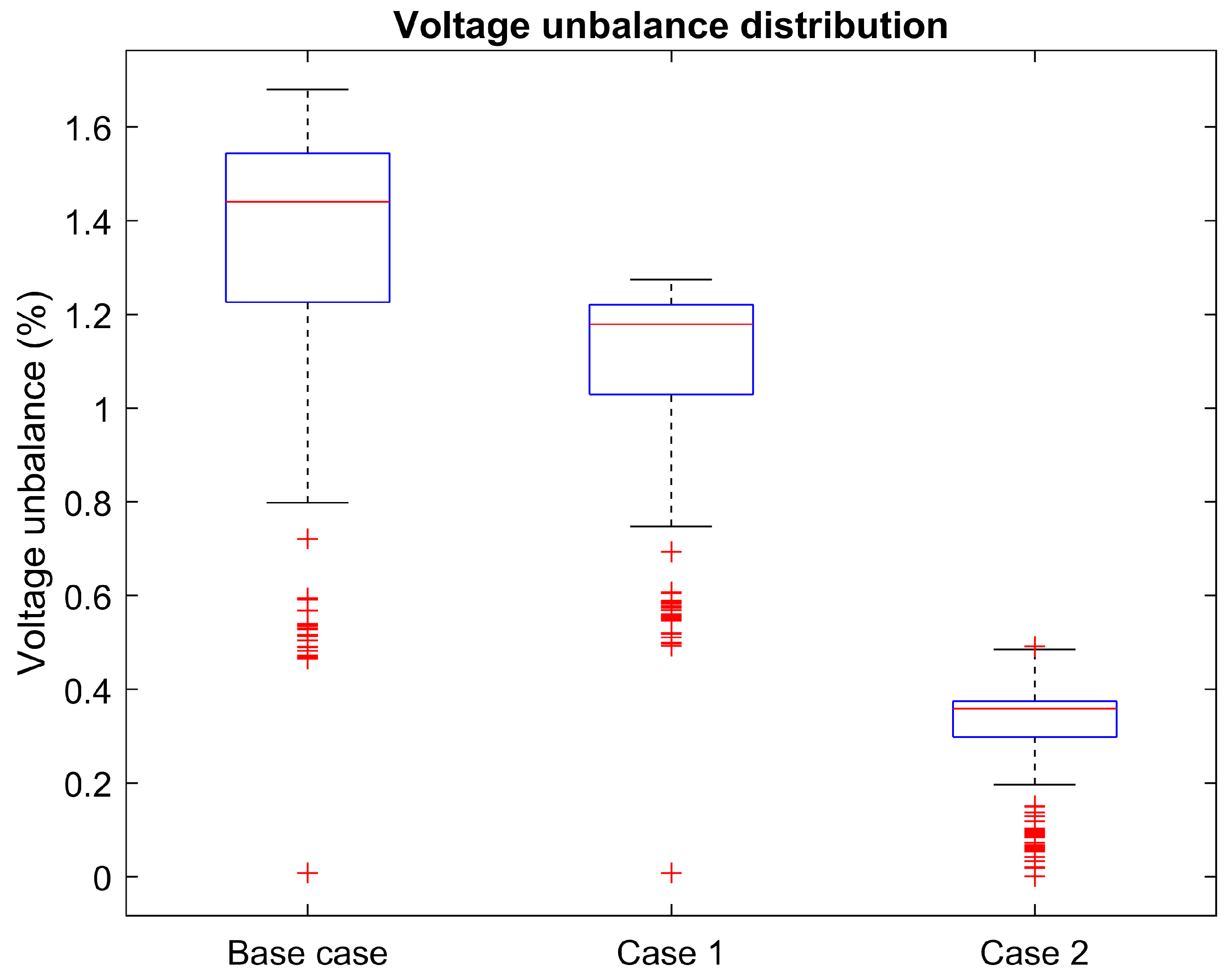
The simulation circuit is a 12 kV distribution feeder of a utility. The one-line diagram is plotted in Figure 19 using GridPV tool [20]. This feeder is served by a 25 MVA, 69/12 kV, wye-wye connected substation transformer. The circuit has unbalanced loads of 2795, 3216, 3260 kW, in phases A, B, and C, respectively. Additionally, there are 215 single-phase PVs generating a total power of 1806, 916, 716 kW, in phases A, B, and C, respectively. With loads and PVs connected, the total power at the feeder head is 953.4 + j 692, 2369.8 + j 1104.5, 2572.6 + j 1152.6 kVA as shown in Figure 20a. It can be observed that this power unbalance is the result of the lightly loaded conditions and high PV penetration in Phase A in comparison to the other phases. The distribution of the voltage unbalance of all buses is shown in Figure 21 under “base case” scenario. Voltage unbalance of most buses is in the range 0.8–1.6% with an average of 1.2%. A few buses have voltage unbalance below 0.8%. These buses are located near the substation where voltage is balanced. In general, it can be observed that the farther away from the feeder head, the higher the voltage unbalance.
For IPPF control application demonstration purpose, it is assumed that there are 130 single-phase power electronic interfaces connected across each A-B and A-C phase. These devices can inject or absorb 12 kvar for IPPF control application. In addition, 5150-kvar capacitor banks across A-C phase are assumed to be connected at the primary feeder. These capacitor banks can be used in conjunction with the power electronic interfaces to share the IPPF control burden.
4.2.2. Interphase Power Flow Control
Three scenarios are considered for evaluating the IPPF control. The first scenario, “base case”, is the original feeder without IPPF control. This scenario will serve as the baseline for comparison.
In the second scenario, denoted “Case 1”, a simple IPPF control is implemented for routing active power from phase A to phase B and C so that the active power is balanced at the feeder head. The total reactive power requirement for IPPF application is calculated using (12). This reactive power burden is then shared evenly among all IPPF control devices; 10.4, −10.7 and 150 kvar is required from each A-B and A-C phase IPPF control device and capacitor bank, respectively.
The third scenario, denoted “Case 2”, has IPPF control implemented the same as Case 1. In addition, the existing PVs are utilized for power factor correction so that power factor is unity at the feeder head. The reactive power requirement for power factor correction is calculated from the result of Case 1 and shared evenly among the PVs.
4.2.3. Simulation Results
The active and reactive power at the feeder head and the voltage unbalance distribution of all scenarios are summarized in Table 1 and Figure 21, respectively. In Case 1, the power at the feeder head becomes 1988.7 + j 366, 1906.1 + j 1767.3, and 1926.3 − j 32.1 kVA in phase A, B, and C, respectively. The system loss is reduced by 4%. The active power becomes balanced as expected after IPPF control. The reactive power is reduced in phase A and C, while increased in phase B. The reactive power remains unbalanced as it is not controlled and utilized for active power routing.
As observed in Figure 21, the average voltage unbalance is reduced from base case to 1%. Furthermore, significant voltage unbalance reduction is observed for the buses further away from the substation (voltage unbalance greater than 50th percentile). This demonstrates the effectiveness of performing unbalanced compensation in a distributive manner. Power unbalance is compensated throughout the system and voltage unbalance is improved throughout the system rather than a few locally.
In Case 2, the substation power after power routing is as shown in Figure 20b. Both active and reactive power at the feeder head becomes balanced: 1980 − j 11.2, 1944.9 − j 90.7, 1955.2 − j 9.8 kVA in phase A, B, and C, respectively. Significant improvement can be observed in system loss and voltage unbalance. System loss is reduced by 14% while the average voltage unbalance is reduced to 0.2%. Compared to Case 1, balance in both active and reactive power is achieved by using the line-to-neutral PVs to complement the IPPF control devices. The line-to-neutral PVs help compensate the reactive power in each phase which is not controlled in the IPPF control.
The simulation in this section demonstrates the effectiveness of the simple IPPF control in balancing the active power at the feeder head. The resulting system shows improvement in both voltage unbalance and system loss. The voltage unbalance of all buses show improvement rather than a few locally as the unbalance compensation is performed in a distributed manner throughout the circuit. Moreover, the line-to-neutral devices can be utilized to control or compensate the reactive power which is regulated in the active power routing. With both IPPF control and power factor correction, significant voltage unbalance and system loss is observed.
5. Conclusions
In this work, the power flow phenomena of single-phase elements were investigated and modeled as IPPF. The analysis showed that IPPF can be decomposed into three components: the fundamental power of the single-phase elements which is drawn equally from each terminal, the IPPR caused by voltage unbalance, and IPPR caused by the presence of the opposite power quantity. The last component is the key that enables IPPF controls for (1) line-to-line single-phase elements and (2) line-to-neutral single-phase elements that are connected at the wye side of delta-wye transformers.
Based on the developed model, the control for line-to-line SVCs and power electronic interfaces was proposed for achieving a desired IPPR or IPPF. For SVCs, the determination of the appropriate reactive power and reactance for achieving the desired power routing was proposed. For the power electronic interfaces, two operation modes along with the hierarchical controls were proposed. In the first mode, the total power of the power electronic interfaces is controlled. In the second mode, ancillary functions including precise power injection and interphase power routing control were developed.
The developed models and control effectiveness were verified and demonstrated through two simulations. In the multimicrogrid system simulation, IPPF control was implemented to improve system operations and flexibility by directing the active power from a phase of a microgrid to the desired device in another phase of another microgrid. The main active power operations of the controlled devices are not interrupted while the devices are utilized for IPPF control. Furthermore, the control burden can be shared among multiple participants for distributed control. In the second simulation, a simple IPPF control was applied to a utility distribution circuit to balance the active power at the feeder head. Results showed reductions in both system voltage unbalance and losses.
Future work should explore improved coordination for IPPF controls to further enhance the operation and resiliency of distribution systems and microgrids. In addition to the line-to-line single-phase elements, other devices should be investigated for potential IPPF control utilization. The performance of the future IPPF controls should be improved with more complex dispatch schemes. Reactive power routing and limitations of IPPF devices such as energy and power availability should be considered.
Author Contributions
Conceptualization, P.S., S.S.; Validation, P.S., V.C.C.; Writing—original draft, P.S.; Writing—review and editing, N.G.B., S.S., V.C.C. All authors have read and agreed to the published version of the manuscript.
Funding
This work was supported in part by Sao Paulo Research Foundation (FAPESP) grants 2017/10476-3, 2019/20186-8 and 2016/08645-9.
Institutional Review Board Statement
Not applicable.
Informed Consent Statement
Not applicable.
Data Availability Statement
No new data were created or analyzed in this study. Data sharing is not applicable to this article.
Conflicts of Interest
The authors declare no conflict of interest.
Abbreviations
The following abbreviations are used in this manuscript:
| DER | Distributed energy resource |
| DSRF | Double synchronous reference frame |
| DSTATCOM | Distribution static compensator |
| ES | Energy storage |
| FACT | Flexible alternating current transmission system |
| IPPF | Interphase power flow |
| IPPR | Interphase power routing |
| MC | Microgrid |
| P | Active power |
| PLL | Phase lock loop |
| PV | Photovoltaic |
| Q | Reactive power |
| S | Complex power |
| SOGI-QSG | Second-order-general integrator quadrature signal generator |
| SVC | Static var compensator |
References
- Chembe, D. Reduction of power losses using phase load balancing method in power networks. In Proceedings of the World Congress on Engineering and Computer Science (WCECS), San Francisco, CA, USA, 20–22 October 2009; pp. 492–497. [Google Scholar]
- Sahito, A.; Memon, Z.; Shaikh, P.; Ahmed Rajper, A.; Memon, S. Unbalanced loading; An overlooked contributor to power losses in HESCO. Sindh Univ. Res. J. Sci. Ser. 2016, 47, 779–782. [Google Scholar]
- Ghosh, A.; Joshi, A. A new approach to load balancing and power factor correction in power distribution system. IEEE Trans. Power Deliv. 2000, 15, 417–422. [Google Scholar] [CrossRef]
- Czarnecki, L.S.; Haley, P.M. Unbalanced power in four-wire systems and its reactive compensation. IEEE Trans. Power Deliv. 2015, 30, 53–63. [Google Scholar] [CrossRef]
- Quintela, F.; Arévalo, J.; Redondo, R.; Melchor, N. Four-wire three-phase load balancing with Static VAr Compensators. Int. J. Electr. Power Energy Syst. 2011, 33, 562–568. [Google Scholar] [CrossRef]
- Jiang, I.H.; Nam, G.; Chang, H.; Nassif, S.R.; Hayes, J. Smart grid load balancing techniques via simultaneous switch/tie-line/wire configurations. In Proceedings of the IEEE/ACM International Conference on Computer-Aided Design (ICCAD), San Jose, CA, USA, 3–6 November 2014; pp. 382–388. [Google Scholar]
- Haq, S.U.; Arif, B.; Khan, A.; Ahmed, J. Automatic three phase load balancing system by ssing fast switching relay in three phase distribution system. In Proceedings of the 1st International Conference on Power, Energy and Smart Grid (ICPESG), Mirpur, Pakistan, 12–13 April 2018; pp. 1–6. [Google Scholar]
- Chang, T.H.; Lee, T.E.; Lin, C.H. Distribution network reconfiguration for load balancing with a colored petri net algorithm. In Proceedings of the 2017 ICASI, Sapporo, Japan, 13–17 May 2017; pp. 1040–1043. [Google Scholar]
- Mayordomo, J.G.; Izzeddine, M.; Asensi, R. Load and voltage balancing in harmonic power flows by means of Static VAr Compensators. IEEE Trans. Power Deliv. 2002, 17, 761–769. [Google Scholar] [CrossRef]
- Mishra, M.K.; Ghosh, A.; Joshi, A.; Suryawanshi, H.M. A novel method of load compensation under unbalanced and distorted voltages. IEEE Trans Power Deliv. 2007, 22, 288–295. [Google Scholar] [CrossRef] [Green Version]
- Singh, B.; Solanki, J. A comparison of control algorithms for DSTATCOM. IEEE Trans. Ind. Electron. 2009, 56, 2738–2745. [Google Scholar] [CrossRef]
- Arya, S.R.; Singh, B.; Niwas, R.; Chandra, A.; Al-Haddad, K. Power quality enhancement using DSTATCOM in distributed power generation system. IEEE Trans. Ind. Appl. 2016, 52, 5203–5212. [Google Scholar] [CrossRef]
- Chang, W.; Liao, C.; Wang, P. Unbalanced load dompensation in three-phase power system with a current-regulared dstatcom based on multilevel converter. J. Mar. Sci. Technol. 2016, 24, 484–492. [Google Scholar]
- Tenti, P.; Trombetti, D.; Tedeschi, E.; Mattavelli, P. Compensation of load unbalance, reactive power and harmonic distortion by cooperative operation of distributed compensators. In Proceedings of the 2009 13th European Conference on Power Electronics and Applications, Barcelona, Spain, 8–10 September 2009; pp. 1–10. [Google Scholar]
- Mousazadeh Mousavi, S.Y.; Jalilian, A.; Savaghebi, M.; Guerrero, J.M. Flexible compensation of voltage and current unbalance and harmonics in microgrids. Energies 2017, 10, 1568. [Google Scholar] [CrossRef]
- El-Naggar, A.; Erlich, I. Control approach of three-phase grid connected PV inverters for voltage unbalance mitigation in low-voltage distribution grids. IET Renew. Power Gener. 2016, 10, 1577–1586. [Google Scholar] [CrossRef]
- Hong, T.; de León, F. Controlling non-synchronous microgrids for load balancing of radial distribution systems. IEEE Trans. Smart Grid 2017, 8, 2608–2616. [Google Scholar] [CrossRef]
- Tang, F.; Zhou, J.; Xin, Z.; Huang, S.; Loh, P.C. An improved three-phase voltage source converter with high-performance operation under unbalanced conditions. IEEE Access 2018, 6, 15908–15918. [Google Scholar] [CrossRef]
- Ciobotaru, M.; Teodorescu, R.; Blaabjerg, F. A new single-phase PLL structure based on second order generalized integrator. In Proceedings of the 2006 37th IEEE Power Electronics Specialists Conference, Jeju, Korea, 18 June 2006; pp. 1–6. [Google Scholar]
- Reno, M.J.; Coogan, K. Grid Integrated Distributed PV (GridPV). Available online: https://www.osti.gov/servlets/purl/1165229 (accessed on 10 January 2015).
Figure 1.
Interphase power flow model of a single-phase load connected across terminal a and b.
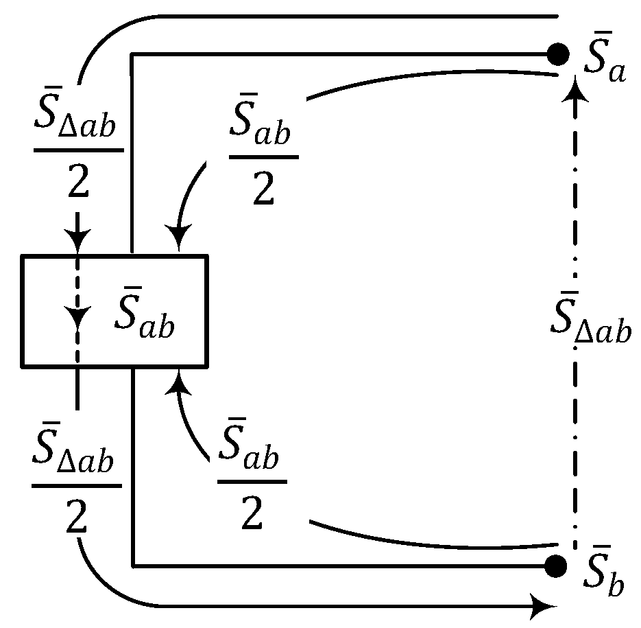
Figure 2.
Physical models of single-phase constant (a) current, (b) power, (c) impedance loads.
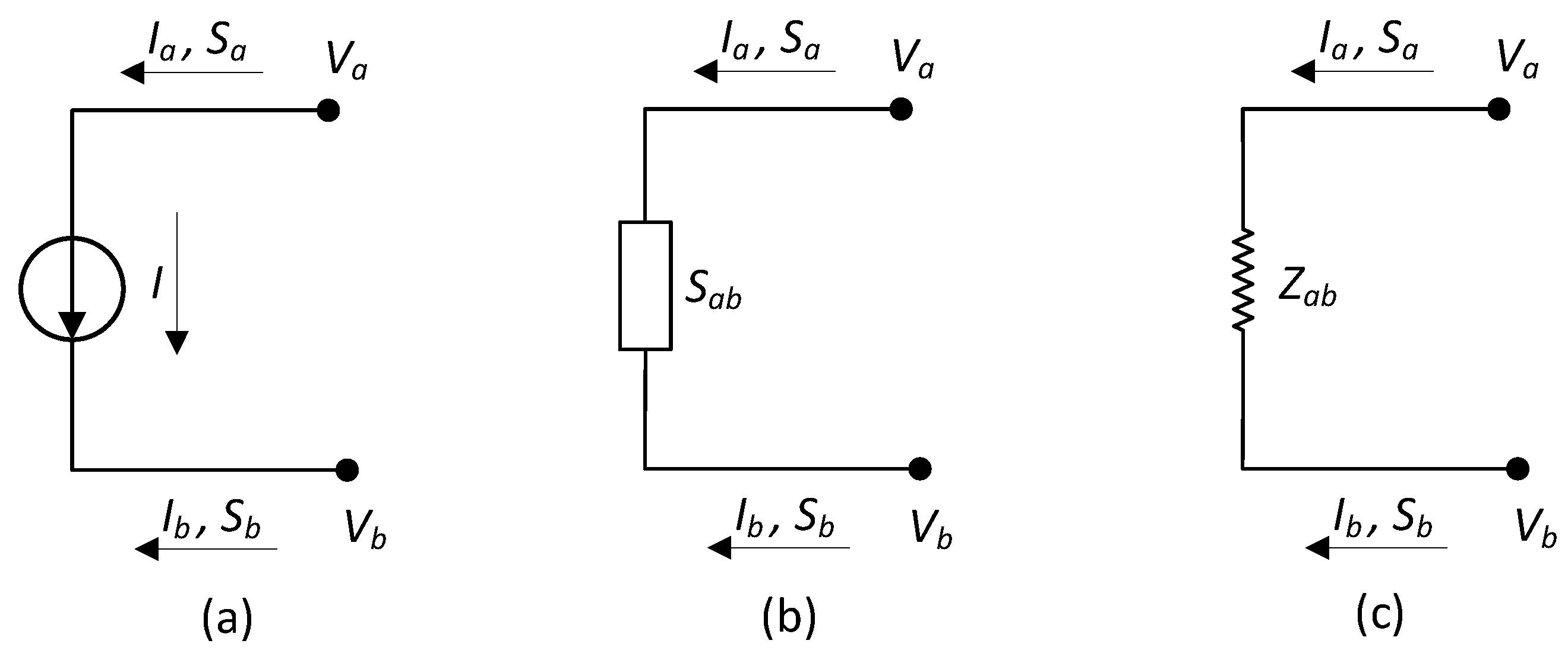
Figure 3.
Interphase power flow of a constant power load.
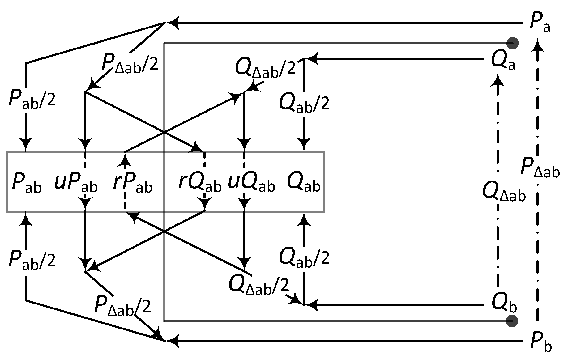
Figure 4.
A circuit diagram of a delta-wye transformer (Dy1) and the IPPF at the delta winding as a result of a phase a load on the wye winding.
Figure 4.
A circuit diagram of a delta-wye transformer (Dy1) and the IPPF at the delta winding as a result of a phase a load on the wye winding.

Figure 5.
Physical model of a single-phase line-to-line power electronic interface.

Figure 6.
Interphase power flow control blocks of power electronic interfaces.
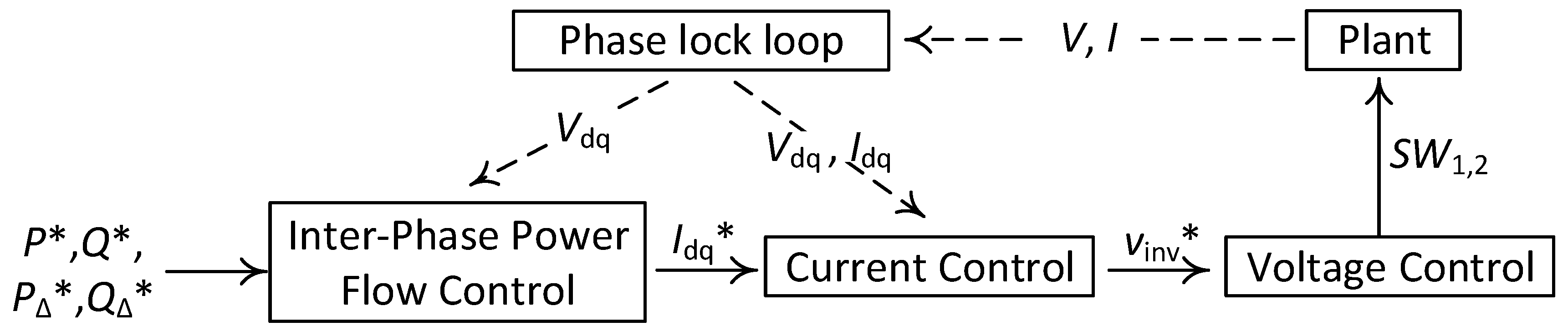
Figure 7.
Second-order-general integrator quadrature signal generator control block.

Figure 8.
Double synchronous reference frame current control block.
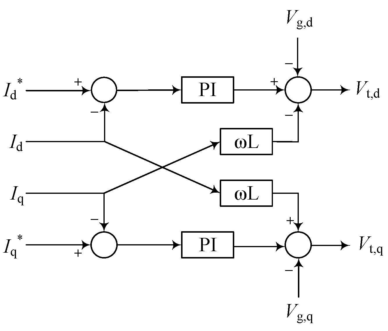
Figure 9.
Multi-microgrid system.

Figure 10.
PSCAD model of the multimicrogrid systems. The multimeters display the initial active and reactive power flow (in kW and kvar) of the circuit with no power injection from PVs and ESs.
Figure 10.
PSCAD model of the multimicrogrid systems. The multimeters display the initial active and reactive power flow (in kW and kvar) of the circuit with no power injection from PVs and ESs.
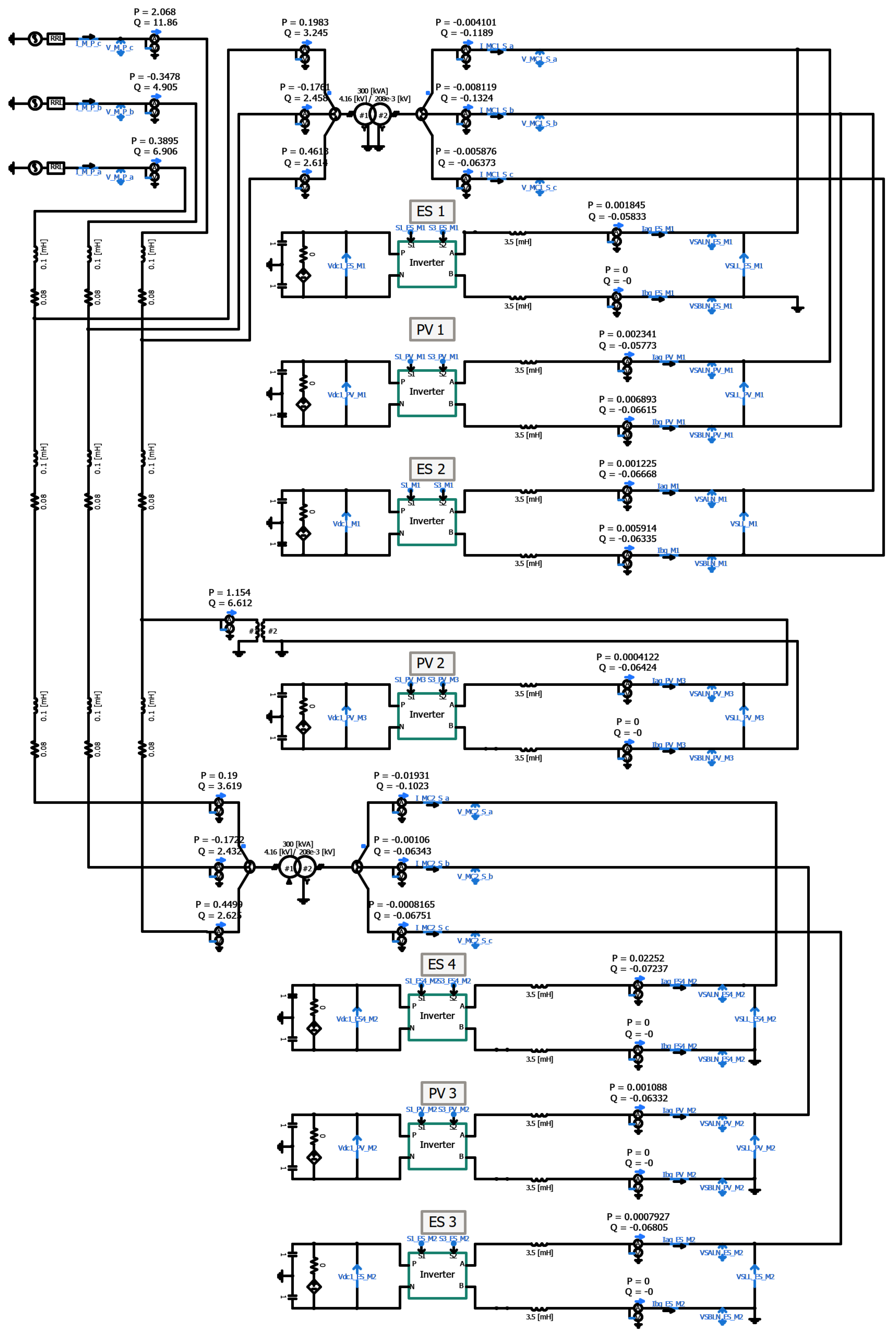
Figure 11.
Theoretical interphase active (a) and reactive (b) power flow at the delta-wye transformer (Dy1) of MC2 as a result of routing 10 kW from phase B to C at the secondary circuit. The active and reactive power required for IPPF control are provided solely from the secondary circuit.
Figure 11.
Theoretical interphase active (a) and reactive (b) power flow at the delta-wye transformer (Dy1) of MC2 as a result of routing 10 kW from phase B to C at the secondary circuit. The active and reactive power required for IPPF control are provided solely from the secondary circuit.
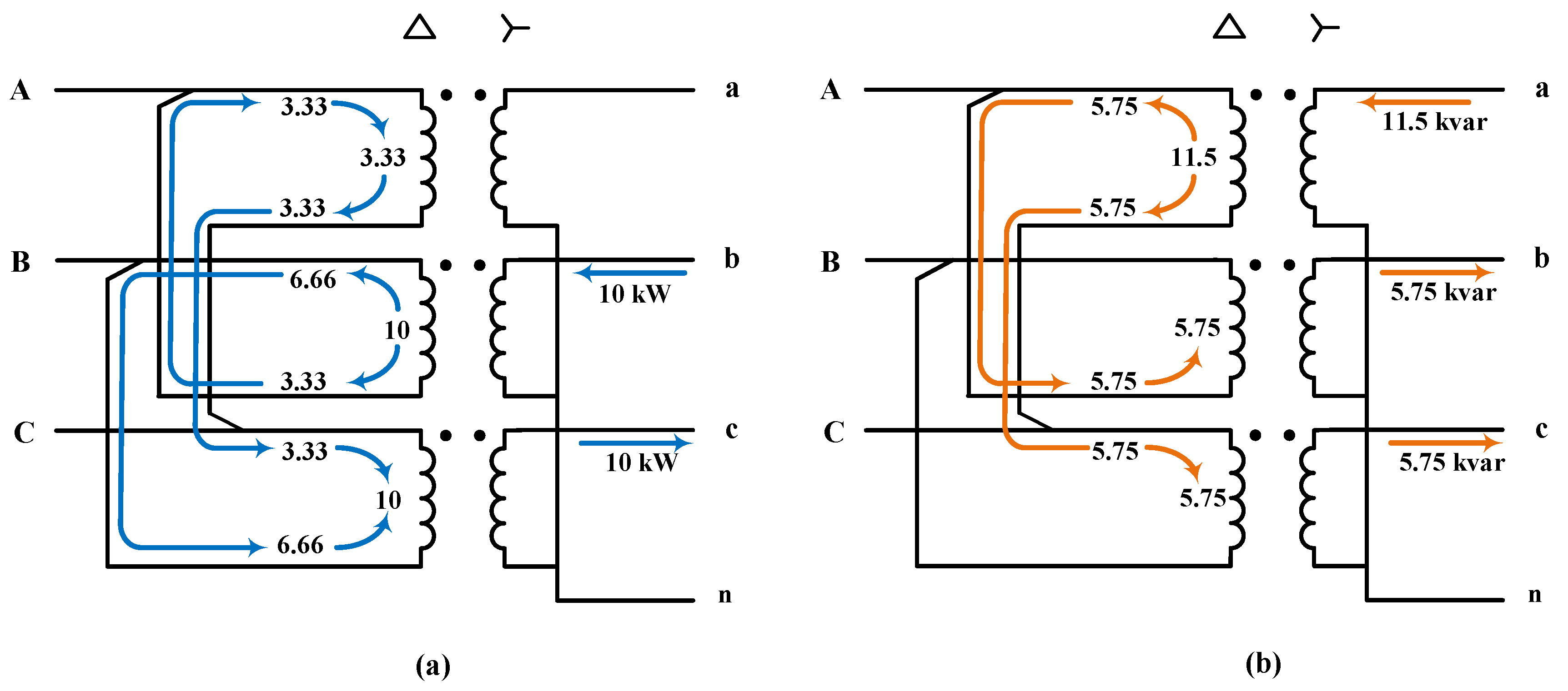
Figure 12.
Feeder head active power shows that the power is shared between the multimicrogrid system effectively without requiring the power from the feeder head.
Figure 12.
Feeder head active power shows that the power is shared between the multimicrogrid system effectively without requiring the power from the feeder head.

Figure 13.
Active power at the wye side at the delta-wye transformer (Dy1) of MC2. Active power in phase A, B and C are labeled as Pa, Pb, Pc, respectively.
Figure 13.
Active power at the wye side at the delta-wye transformer (Dy1) of MC2. Active power in phase A, B and C are labeled as Pa, Pb, Pc, respectively.

Figure 14.
Active power across A-B winding at the delta side of T3. Active power injection to terminal A, B, and total power are labeled as Pa, Pb, Pab, respectively.
Figure 14.
Active power across A-B winding at the delta side of T3. Active power injection to terminal A, B, and total power are labeled as Pa, Pb, Pab, respectively.

Figure 15.
Active power at the secondary side at the wye-wye transformer of MC1. Active power in phase A, B and C are labeled as Pa, Pb, Pc, respectively.
Figure 15.
Active power at the secondary side at the wye-wye transformer of MC1. Active power in phase A, B and C are labeled as Pa, Pb, Pc, respectively.

Figure 16.
Active power of PV1 in MC1. Active power injection to phase A, B, and total power are labeled as Pa, Pb, Pab, respectively.
Figure 16.
Active power of PV1 in MC1. Active power injection to phase A, B, and total power are labeled as Pa, Pb, Pab, respectively.

Figure 17.
PSCAD simulation shows the active and reactive power flow (in kW and kvar) of the multimicrogrid system after all power routing actions. (1) Within MC2, 10 kW from PV3 (phase B) is routed to ES3 (phase C), (2) 10 kW from PV2 in MC3 (phase C) is routed to charge ES2 in MC1 (on phase B-C), and (3) 10 kW from PV3 in MC2 (phase B) and 10 kW from PV1 in MC1 (phase A-B) are routed to charge ES1 in MC1 (phase A).

Figure 18.
PSCAD simulation shows the active and reactive power flow (in kW and kvar) of Microgrid 2 after the first power routing action. 10 kW from phase B is routed to C at the secondary circuit. The active and reactive power required for IPPF control are provided solely from the secondary circuit.

Figure 19.
One-line diagram of the distribution circuit shows the locations of the PVs (PVs), line-to-line power electronic interfaces connected across A-B phase (A-B devices) and C-A phase (C-A devices), and capacitor banks.
Figure 19.
One-line diagram of the distribution circuit shows the locations of the PVs (PVs), line-to-line power electronic interfaces connected across A-B phase (A-B devices) and C-A phase (C-A devices), and capacitor banks.
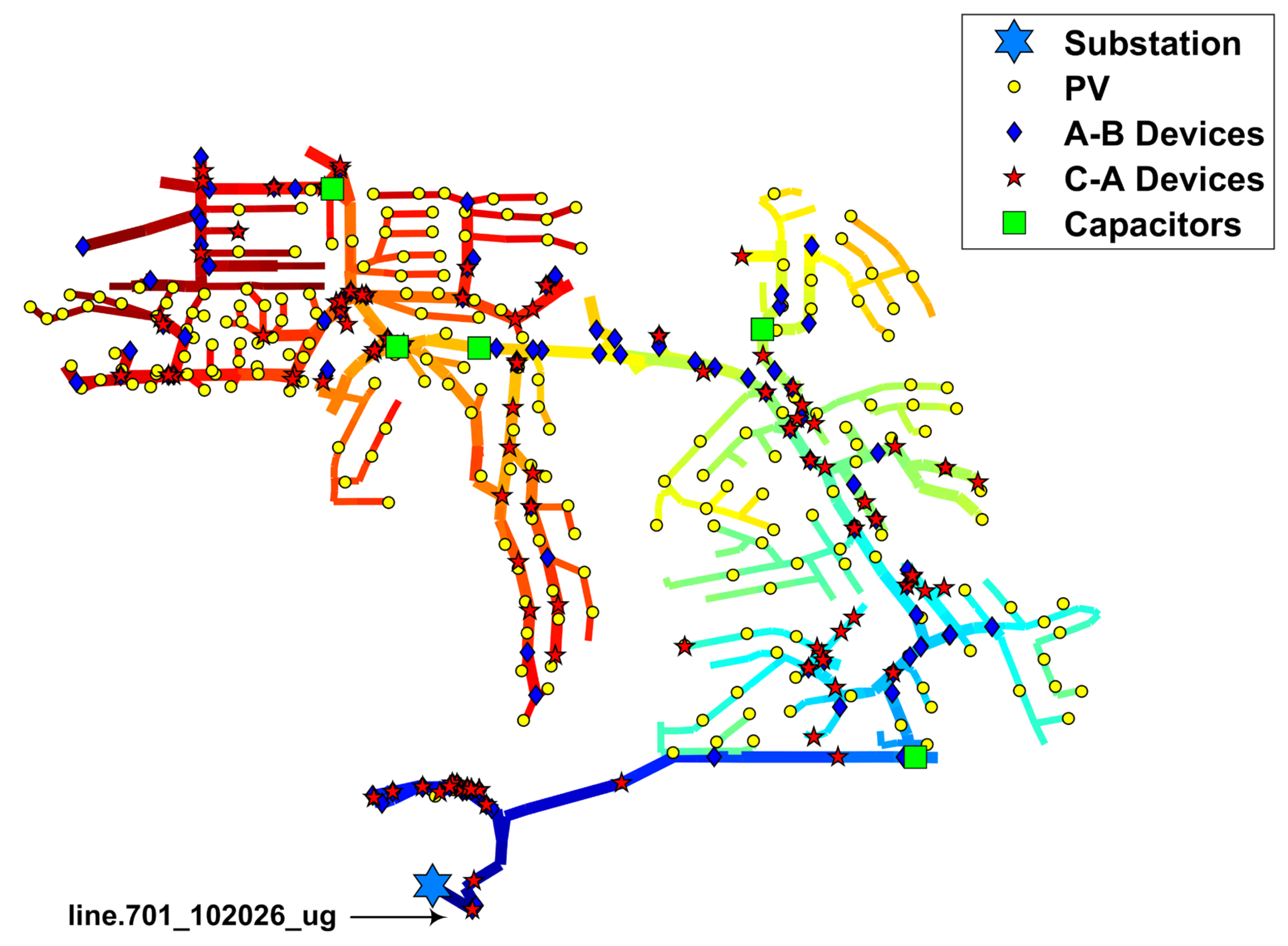
Figure 20.
Substation active and reactive power flow in (a) base case, and (b) Case 2.

Figure 21.
Voltage unbalance distribution of base case, Case 1 with IPPF control, and Case 2 with IPPF control and PF correction.
Figure 21.
Voltage unbalance distribution of base case, Case 1 with IPPF control, and Case 2 with IPPF control and PF correction.

Table 1.
Active and reactive power at the feeder head of base case, Case 1 and Case 2.
| Feeder Head Power | ||||||
|---|---|---|---|---|---|---|
| Scenarios | Active Power (kW) | Reactive Power (kvar) | ||||
| Pa | Pb | Pc | Qa | Qb | Qc | |
| Base case | 953.4 | 2369.8 | 2572.6 | 692 | 1104.5 | 1152.6 |
| Case 1 | 1988.7 | 1906.1 | 1926.3 | 366 | 1767.3 | −32.1 |
| Case 2 | 1980 | 1944.9 | 1955.2 | −11.2 | −90.7 | −9.8 |
Publisher’s Note: MDPI stays neutral with regard to jurisdictional claims in published maps and institutional affiliations. |
© 2021 by the authors. Licensee MDPI, Basel, Switzerland. This article is an open access article distributed under the terms and conditions of the Creative Commons Attribution (CC BY) license (http://creativecommons.org/licenses/by/4.0/).
Share and Cite
MDPI and ACS Style
Siratarnsophon, P.; Cunha, V.C.; Barry, N.G.; Santoso, S. Interphase Power Flow Control via Single-Phase Elements in Distribution Systems. Clean Technol. 2021, 3, 37-58. https://doi.org/10.3390/cleantechnol3010003
AMA Style
Siratarnsophon P, Cunha VC, Barry NG, Santoso S. Interphase Power Flow Control via Single-Phase Elements in Distribution Systems. Clean Technologies. 2021; 3(1):37-58. https://doi.org/10.3390/cleantechnol3010003
Chicago/Turabian StyleSiratarnsophon, Piyapath, Vinicius C. Cunha, Nicholas G. Barry, and Surya Santoso. 2021. "Interphase Power Flow Control via Single-Phase Elements in Distribution Systems" Clean Technologies 3, no. 1: 37-58. https://doi.org/10.3390/cleantechnol3010003