A Practicable Guideline for Predicting the Thermal Conductivity of Unconsolidated Soils

Abstract

For large infrastructure projects, such as high-voltage underground cables or for evaluating the very shallow geothermal potential (vSGP) of small-scale horizontal geothermal systems, large-scale geothermal collector systems (LSCs), and fifth generation low temperature district heating and cooling networks (5GDHC), the thermal conductivity (λ) of the subsurface is a decisive soil parameter in terms of dimensioning and design. In the planning phase, when direct measurements of the thermal conductivity are not yet available or possible, λ must therefore often be estimated. Various empirical literature models can be used for this purpose, based on the knowledge of bulk density, moisture content, and grain size distribution. In this study, selected models were validated using 59 series of thermal conductivity measurements performed on soil samples taken from different sites in Germany. By considering different soil texture and moisture categories, a practicable guideline in the form of a decision tree, employed by empirical models to calculate the thermal conductivity of unconsolidated soils, was developed. The Hu et al. (2001) model showed the smallest deviations from the measured values for clayey and silty soils, with an RMSE value of 0.20 W/(m∙K). The Markert et al. (2017) model was determined to be the best-fitting model for sandy soils, with an RMSE value of 0.29 W/(m∙K).

1. Introduction

The decarbonization of the energy supply in the heating sector is necessary to meet climate targets [1]. Shallow geothermal systems can contribute significantly to achieving these goals. Particularly for very shallow closed-loop systems, as well as regarding heat extraction rates [2], the very shallow geothermal potential (vSGP) in the form of the thermal conductivity of soils (λ) is a decisive factor for efficient performance [3].

In addition to the generation of sustainable geothermal heating and cooling energy for individual residential and industrial buildings, there is also the possibility of using large-scale geothermal collector systems (LSCs) to cover significantly higher energy demands [4,5]. In combination with fifth generation low-temperature district heating and cooling networks (5GDHC), these systems can meet the needs of entire residential areas [5,6,7,8]. Due to the low temperature level and the non-insulated pipes [5] used in these systems, these networks also act as ground heat exchangers; thus, thermal conductivity is also a decisive factor for the energetic performance here.

Another key element of the energy transformation, particularly in regards to the SuedLink project in Germany [9], is the distribution of electricity from the site of production to the consumer over long distances via high-voltage direct current underground cables. The basic requirement for this transformation is that the function of the cables is guaranteed. For this reason, the thermal conductivity of the surrounding subsurface is of major relevance [10], as the heating of the cables due to the lack of heat dissipation determines their durability [11]. For planning such large infrastructure projects, the thermal conductivity of the soil must therefore be considered when estimating the heat dissipation in the cable environment.

The thermal conductivity of unconsolidated soils is mainly influenced by the grain size distribution, bulk density, and moisture content of the soil physical parameters [2,12,13,14]. Direct measurements of λ are often performed in situ or in the laboratory using single-needle sensors [15,16,17,18,19]. For example, Markert et al. [20] proposed an approach for measuring λ in a wide moisture content spectrum based on the evaporation method.

Thermal conductivity measurements in the planning phases of large-scale infrastructure projects such as LSCs, 5HDHC, or high-voltage underground cables are often not possible due to the high effort required or the early stage of the project. However, λ can be calculated using a variety of largely empirical models, if specific soil input parameters are known or assumed [21,22,23,24,25,26,27,28,29,30]. This requires the estimation of the accuracy or error of the model used. For this reason, the aim of this study is to validate selected thermal conductivity models using a variety of laboratory measurement series. In addition, by consideration of subsets with different soil properties regarding grain size distribution or moisture content, a practicable guideline for the use of empirical models for calculating the thermal conductivity of soils can be developed, based on the knowledge of the grain size distribution, bulk density, and moisture content.

The soil properties differ from those of previous validations [31,32,33,34] due to different sampling sites, all in Germany, and the combination of two measurement methods using needle sensors. The selection of empirical thermal conductivity models for validation was based on the work of Wessolek et al. [34], with additional consideration of the model of Markert et al. [27]. Therefore, the selection used in this study also differs from that of Dong et al. [31] and Tarnawski et al. [33]. Moreover, while He et al. [32] only focused on models based on the model of Johansen [35,36], this study also validated models with different basic approaches.

Tarnawski et al. [33] only considered the measured thermal conductivities of soils in dry and saturated conditions, whereas in this study, a wide range of saturations was considered. Furthermore, the detailed consideration of subsets, in terms of moisture and grain size distribution, employing this amount of data and a wider range of model selection in terms of publication periods, was not performed in the previous validations and is therefore novel.

2. Materials and Methods

2.1. Thermal Conductivity Measurement Database Used for Validation

For the validation, a total of 59 measurement series were used. The data are taken from various research projects in Germany of the Shallow Geothermal Energy Working Group from the Friedrich-Alexander-University Erlangen-Nuremberg. A measurement series is defined as a certain number of measurements (measurement points) of the thermal conductivity at specific moisture contents on a soil sample with a defined bulk density, grain size distribution, and measurement method.

The thermal conductivity measurements were performed exclusively with a single-needle sensor. The devices used and their measurement accuracy are listed in

Table 1. Thermal properties analyzer and the specifications used for thermal conductivity measurements.

Thermal Properties Analyzer	Manufacturer	Single-Needle	Accuracy
KD2 Pro	Decagon Devices, Inc. (Pullman, WA, USA)	TR-1 (10 cm)	±10% from 0.2–4.0 W/(m∙K)
Tempos	METER Group, Inc. (Pullman, WA, USA)	TR-3 (10 cm)	±10% from 0.2–4.0 W/(m∙K)

. The configurations of the used single-needle sensors comply with the specifications according to IEEE Std 442-1981 [37] and ASTM D5334 [38].

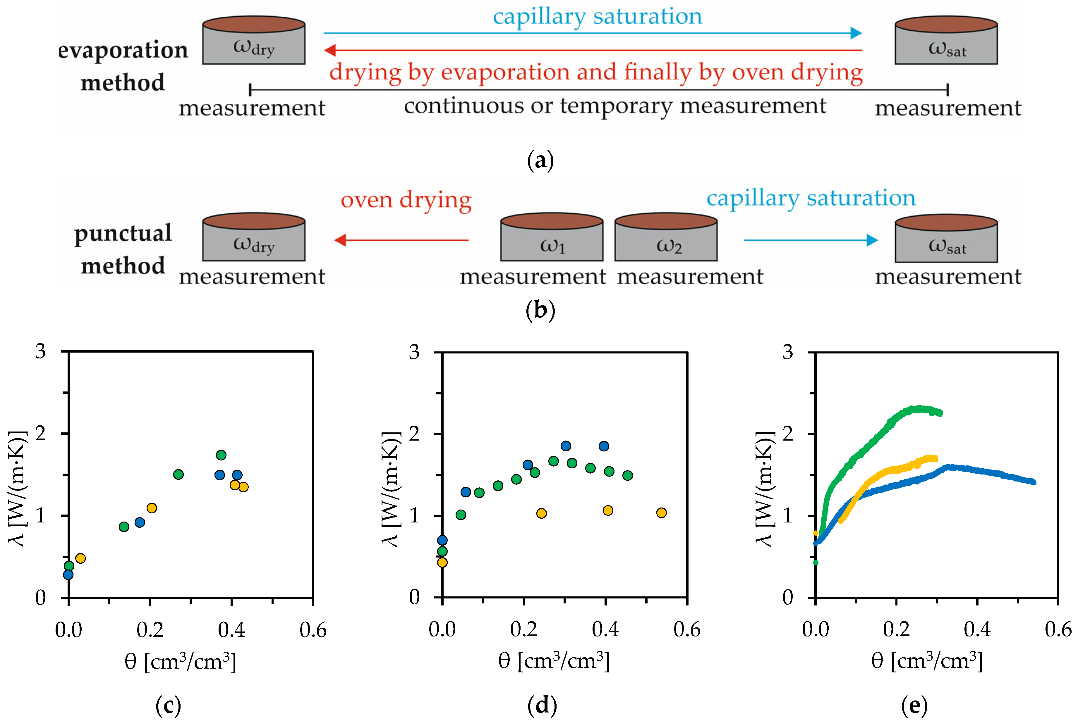
The measurements were carried out using two different methods. These are described in

Table 2. Measurement methods used for the thermal conductivity measurements. For each thermal conductivity measurement, the moisture content was determined. Here, for the number of measurement points per measurement series, the complete water content range is considered.

Number of Measurement Series	Description	Number of Measurement Points per Measurement Series
49	Evaporation method based on the approach of Markert et al. [20], with continuous measurements, obtained at 15 min to 60 min intervals, or temporary measurements, e.g., performed at daily intervals; measurements performed in cylinders.	4–2227
10	Punctual method, as described in the work of Rammler et al. [18]; measurements performed in cylinders.	4

and in Figure 1.

For the evaporation method, oven drying and the measurement of thermal conductivity at a moisture content θ = 0% were not carried out for each sample. In the case of high implausible deviations of λ within one measurement series, the deviating measurement points were removed manually.

All soil samples were installed in the cylinders with volumes of 397 cm³ or 944 cm³ with a specific bulk density using undisturbed sampling. Possible changes in bulk density due to shrinkage and swelling processes during the evaporation method [18,39] were neglected for validation. These changes in density are responsible for the fact that the maximum thermal conductivity in the evaporation method is sometimes not reached at saturation, but rather at an intermediate moisture content. In the case of slightly fluctuating bulk densities in measurement series measured using the punctual method, the average bulk density was assumed for validation. The individual bulk densities deviate from the mean value by a maximum of 0.04 g/cm³.

Due to the different methods or measurement intervals used, the number of measurement points per measurement series varies. However, for the validation, each measurement series was considered equally for authentication, independent of the number of measurement points.

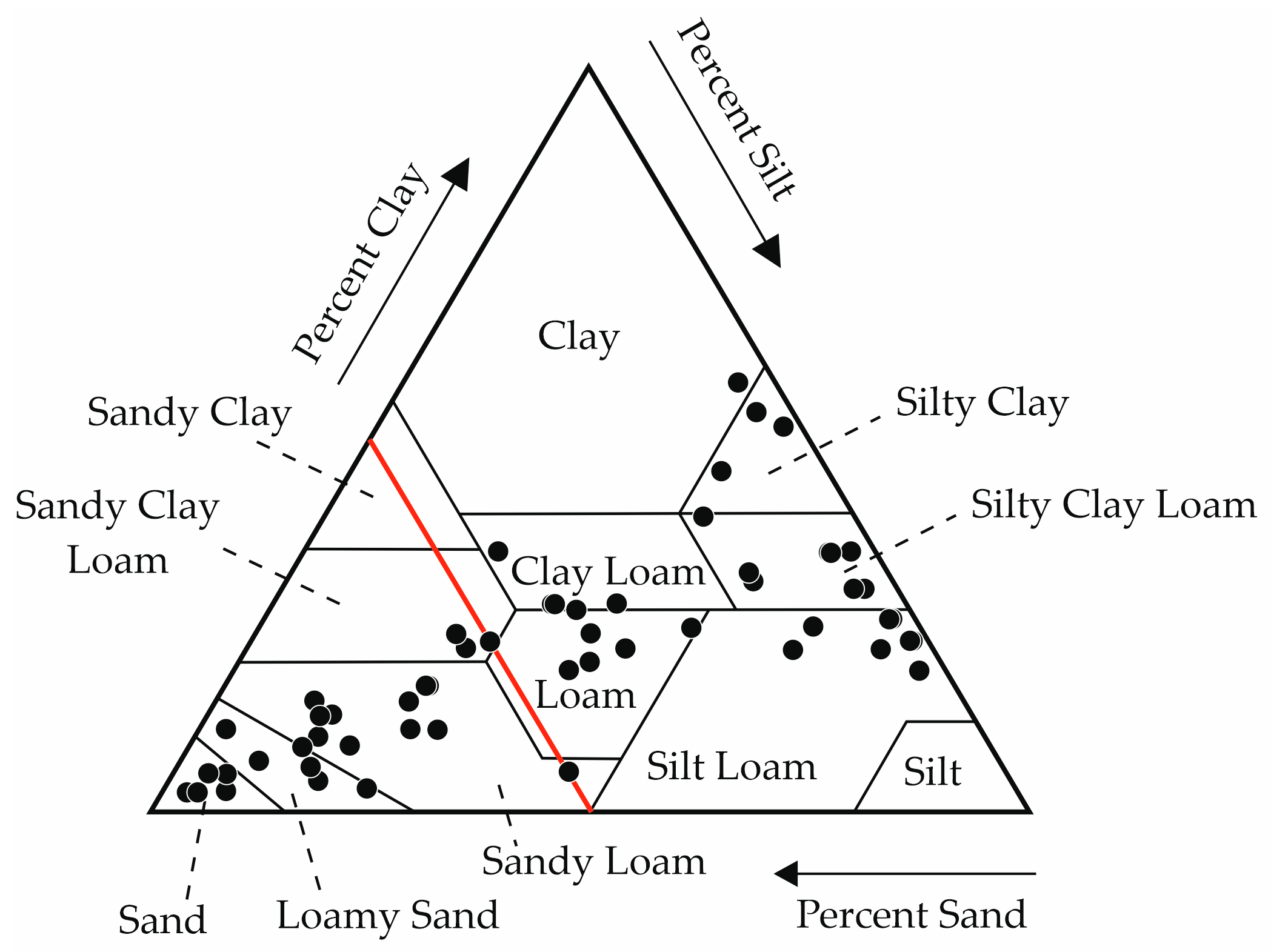
As the measurement series originate from various research projects, the soil samples were taken from different locations in Germany; therefore, a wide range of soil texture classes was covered for the validation (Figure 2). Therefore, only the USDA soil texture classes sandy clay and silt were not considered for the validation. Very occasionally, the soil samples considered are mixed samples, topsoil samples, or anthropogenically influenced soils.

A statistical evaluation of the database regarding the decisive soil parameters is shown in the

Table 3. Statistical analysis of the data base based on the work of Wessolek et al. [34], with λ = thermal conductivity, θ = moisture content, ρ_b = bulk density, S_r = saturation and grain size distributions regarding clay (f_Clay), silt (f_Silt), and sand content (f_Sand). For this overview, the complete water content range is considered here.

	λ [W/(m∙K)]	θ [cm3/cm3]	ρb [g/cm3]	Sr	fClay [%]	fSilt [%]	fSand [%]
Minimum	0.25	0.00	1.15	0.00	3	3	2
1. Quantile	1.17	0.10	1.39	0.22	7	15	12
Median	1.42	0.19	1.47	0.40	19	27	50
Mean	1.41	0.20	1.46	0.43	18	35	47
3. Quantile	1.63	0.28	1.51	0.61	25	60	74
Maximum	2.71	0.64	1.92	1.00	58	78	95

.

2.2. Approach for Validation of Selected Empirical Literature Models

For the validation, the focus was on two key indicators that demonstrate the match between the thermal conductivities calculated using the literature models and the measured values. Therefore, the RMSE (root mean square error) and the bias value were used as follows:

$$\mathrm{R}\mathrm{M}\mathrm{S}\mathrm{E}=\sqrt{\frac{\sum {({\mathsf{\lambda }}_{\mathrm{c}\mathrm{a}\mathrm{l}\mathrm{c}\mathrm{u}\mathrm{l}\mathrm{a}\mathrm{t}\mathrm{e}\mathrm{d}}-{\mathsf{\lambda }}_{\mathrm{m}\mathrm{e}\mathrm{a}\mathrm{s}\mathrm{u}\mathrm{r}\mathrm{e}\mathrm{d}})}^2}{\mathrm{n}}}$$

(1)

$$\mathrm{b}\mathrm{i}\mathrm{a}\mathrm{s}=\frac{\sum ({\mathsf{\lambda }}_{\mathrm{c}\mathrm{a}\mathrm{l}\mathrm{c}\mathrm{u}\mathrm{l}\mathrm{a}\mathrm{t}\mathrm{e}\mathrm{d}}-{\mathsf{\lambda }}_{\mathrm{m}\mathrm{e}\mathrm{a}\mathrm{s}\mathrm{u}\mathrm{r}\mathrm{e}\mathrm{d}})}{\sum {\mathsf{\lambda }}_{\mathrm{c}\mathrm{a}\mathrm{l}\mathrm{c}\mathrm{u}\mathrm{l}\mathrm{a}\mathrm{t}\mathrm{e}\mathrm{d}}}$$

(2)

The RMSE corresponds to the absolute error or deviation. Squaring the deviation prevents positive and negative deviations from neutralizing each other. The bias value corresponds to an average deviation. Here, positive and negative deviations neutralize each other; thus, a negative value indicates that a literature model underestimates the thermal conductivity, on average, compared to measured values. A positive value indicates an overestimation.

For the validation, the RMSE and the bias values were determined for each measurement series based on their measurement points (n). The values of both key indicators were then averaged for all measurement series. As a result, the measurement series were considered equivalent, regardless of their number of measurement points.

For the overall analysis, all measurement series were considered regardless of any soil properties. In addition, for the development of a practicable guideline, the measurement series were divided into two categories according to their grain size distribution, specifically their sand content (f_sand). The subdivision was based on the work of Kersten [25]. A distinction was made between clay and silt soils, with a sand content f_Sand ≤ 50%, and sandy soils, with f_Sand > 50% (

Table 4. Soil properties of the subsets considered in the validation with regard to soil texture and moisture, as well as their designation used for the specific soil texture categories.

Soil Properties		Designation	Number of Measurement Series
fSand	Sr
≤50%	-	Clay and Silt (T/U)	34
	≤50%	Dry Clay and Silt (T/U)	29
	>50%	Moist Clay and Silt (T/U)	34
>50%	-	Sand (S)	25
	≤50%	Dry Sand (S)	24
	>50%	Moist Sand (S)	25

). Furthermore, the validation of the two soil texture categories was also carried out regarding the moisture content. For this differentiation, only measurement points in the measurement series with saturation degrees S_r ≤ 0.5 were considered for dry conditions. For moist conditions, only measurement points with S_r > 0.5 were used. The calculation of the saturation is described in Equation (4).

To ensure comparability, measuring points in the very dry range were not included in the validation, in accordance with the validity limits of the model suggested by Kersten [25]. Therefore, for clay and silty soils, only the measured values with a gravimetric water content w ≥ 7% were used, and for sandy soils, only the measured values with w ≥ 1% were employed. As a result, in some cases the number of measuring points described in Table 2 was reduced.

As the aim was to develop a practical guideline for the use of literature models for calculating thermal conductivity, the evaluation focused mainly on the models showing the smallest deviations from the measured values.

2.3. Validated Models for Calculating Thermal Conductivity

The basic principle for the selection of the calculation models was that not more than the basic soil input parameters of grain size distribution, bulk density, and moisture content must be known, or the parameters derived from and the equations will not contain any free parameters. The selection was based on the models used by Wessolek et al. [34].

From the basic input parameters, the porosity (Φ) and saturation (S_r) were calculated as follows, assuming a particle density (ρ_p) of 2.65 g/cm³:

$$\mathsf{\Phi }=1-\frac{{\mathsf{\rho }}_{\mathrm{b}}}{{\mathsf{\rho }}_{\mathrm{p}}}$$

(3)

Φ = porosity [-]

ρ_b = bulk density [g/cm³]

ρ_p = particle density [g/cm³]

$${\mathrm{S}}_{\mathrm{r}}=\frac{\mathsf{\theta }}{\mathsf{\Phi }}$$

(4)

S_r = saturation [-]

θ = volumetric water content or moisture content [-]

In some cases, the calculated maximum saturation of a measurement series can be greater than 1.0, e.g., due to a deviating particle density or swelling processes within the course of the evaporation method. In these cases, the maximum measured volumetric water content of the measurement series is set as the porosity.

Various models differentiate between fine and sandy soils. Unless otherwise stated, fine-grained soils were defined with a sand content of ≤50%.

The quartz content is calculated according to the method of Hu et al. [41]:

$$\mathrm{q}=0.5{\mathrm{f}}_{\mathrm{s}\mathrm{a}\mathrm{n}\mathrm{d}}$$

(5)

q = quartz content [-]

f_sand = sand content [-]

For the validation, the Python programming language (Python Software Foundation, v3.11) was used. The script can be downloaded at https://github.com/wehnsdaefflae/fusl (accessed on 16 April 2024).

In the following section, the selected models are described in detail.

2.3.1. Kersten (1949) Model

With the model proposed by Kersten [25], for the calculation of the thermal conductivity, only the parameters of bulk density and gravimetric water content are required. Furthermore, the soils are divided into two categories, depending on their sand content (fine textured soils with f_Sand ≤ 50% and granular soils with f_Sand > 50%). Thus, the knowledge of the exact grain size distribution is not required.

In the work of Kersten [25], the equations are given in imperial units. Farouki [14] has rewritten these with a conversion factor for metric units.

For fine-grained soils, the thermal conductivity for w ≥ 7% is calculated as follows:

$$\mathsf{\lambda }=0.1442(0.9\log \mathrm{w}-0.2)\times {10}^{0.6243{\mathsf{\rho }}_{\mathrm{b}}}$$

(6)

λ = thermal conductivity [W/(m∙K)]

w = gravimetric water content [%]

Thermal conductivity is calculated as follows for granular soils of w ≤ 1%:

$$\mathsf{\lambda }=0.1442(0.7\log \mathrm{w}+0.4)\times {10}^{0.6243{\mathsf{\rho }}_{\mathrm{b}}}$$

(7)

2.3.2. Johansen (1975) Model

Johansen [35,36] proposed a new model for calculating the λ of partial saturated soils as a function of the thermal conductivity in both the dry and saturated state. The thermal conductivity between these is interpolated using the degree of saturation and a normalized thermal conductivity (Kersten’s number):

$$\mathsf{\lambda }=\mathrm{K}\mathrm{e}\left({\mathsf{\lambda }}_{\mathrm{s}\mathrm{a}\mathrm{t}}-{\mathsf{\lambda }}_{\mathrm{d}\mathrm{r}\mathrm{y}}\right)+{\mathsf{\lambda }}_{\mathrm{d}\mathrm{r}\mathrm{y}}$$

(8)

λ_sat = thermal conductivity of saturated soil [W/(m∙K)]

λ_dry = thermal conductivity of dry soil [W/(m∙K)]

Ke = Kersten’s number [-]

For coarse soils, which are defined by f_Clay ≤ 5%, the Kersten’s number can be calculated for S_r > 0.05, as follows:

$$\mathrm{K}\mathrm{e}=0.7\log {\mathrm{S}}_{\mathrm{r}}+1$$

(9)

In this study, Ke = 0 was assumed when S_r < 0.05.

For fine soils, which are defined by f_Clay > 5%, Ke can be calculated for the range where S_r > 0.1, as follows:

$$\mathrm{K}\mathrm{e}=\log {\mathrm{S}}_{\mathrm{r}}+1$$

(10)

In the case of S_r < 0.1, in this study, Ke = 0 was assumed.

The calculation of the thermal conductivity of saturated and dry soils is described in Equations (11)–(13). Johansen [35] assumed a value of 0.57 W/(m∙K) for the thermal conductivity of water. The thermal conductivity of quartz is assumed to be 7.7 W/(m∙K). The remaining solid components have a thermal conductivity of 2.0 W/(m∙K). For quartz contents lower than 20%, a thermal conductivity of 3.0 W/(m∙K) is set for the remaining components.

$${\mathsf{\lambda }}_{\mathrm{s}\mathrm{a}\mathrm{t}}={{\mathsf{\lambda }}_{\mathrm{w}}}^{\mathsf{\Phi }}\times {{\mathsf{\lambda }}_{\mathrm{s}}}^{(1-\mathsf{\Phi })}$$

(11)

$${\mathsf{\lambda }}_{\mathrm{s}}={{\mathsf{\lambda }}_{\mathrm{q}}}^{\mathrm{q}}\times {{\mathsf{\lambda }}_{\mathrm{o}}}^{(1-\mathrm{q})}$$

(12)

$${\mathsf{\lambda }}_{\mathrm{d}\mathrm{r}\mathrm{y}}=\frac{0.137{\mathsf{\rho }}_{\mathrm{b}}+64.7}{{\mathsf{\rho }}_{\mathrm{p}}-0.947{\mathsf{\rho }}_{\mathrm{b}}}$$

(13)

λ_w = thermal conductivity of water [0.57 W/(m∙K)]

λ_s = thermal conductivity of solid particles [W/(m∙K)]

λ_q = thermal conductivity of quartz [7.7 W/(m∙K)]

λ_o = thermal conductivity of solid particles [2.0 or 3.0 W/(m∙K)]

ρ_p = particle density [2700 kg/m³]

2.3.3. Brakelmann (1984) Model

The model of Brakelmann [10] is based on experimental results. The thermal conductivity is calculated as follows:

$$\mathsf{\lambda }={{\mathsf{\lambda }}_{\mathrm{w}}}^{\mathsf{\Phi }}\times {{\mathsf{\lambda }}_{\mathrm{s}}}^{(1-\mathsf{\Phi })}\times \mathrm{e}\mathrm{x}\mathrm{p}(-3.08{\left(1-{\mathrm{S}}_{\mathrm{r}}\right)}^2\times \mathsf{\Phi })$$

(14)

λ_w = thermal conductivity of water [0.588 W/(m∙K)]

For the calculation of λ_s, the approach described in Wessolek et al. [34] is used in this study:

$${\mathsf{\lambda }}_{\mathrm{s}}=0.0812{\mathrm{f}}_{\mathrm{s}\mathrm{a}\mathrm{n}\mathrm{d}}+0.054{\mathrm{f}}_{\mathrm{s}\mathrm{i}\mathrm{l}\mathrm{t}}+0.02{\mathrm{f}}_{\mathrm{c}\mathrm{l}\mathrm{a}\mathrm{y}}$$

(15)

f_silt = silt content [%]

f_clay = clay content [%]

2.3.4. Ewen and Thomas (1987) Model

Based on the Johansen (1975) model, Ewen and Thomas [23] proposed a new approach for calculation of Kersten’s number. The original Kersten’s number, according to Johansen [35], cannot be applied for dry soils. In the approach of Ewen and Thomas [23], this was changed using Equation (16), and a new parameter with the value of −8.9 was obtained:

$$\mathrm{K}\mathrm{e}=1-\mathrm{e}\mathrm{x}\mathrm{p}\left(\mathsf{\xi }{\mathrm{S}}_{\mathrm{r}}\right)$$

(16)

ξ = fitted parameter of Ewen and Thomas (1987) model [−8.9]

The further calculation steps correspond to those of the Johansen (1975) model, as shown in Equations (8) and (11)–(13). For Equation (12), a value of 2.0 W/(m∙K) is used for the thermal conductivity of all minerals other than quartz.

Markle et al. [28] expanded the Ewen and Thomas (1987) model and used ξ as a fitting parameter. However, this model was not considered for validation, as it contains a free parameter.

2.3.5. Hu et al. (2001) Model

With the approach of Hu et al. [24], the thermal conductivity of unconsolidated porous media is calculated based on the Johansen (1975) model and the Leverett–Lewis equation for the relationship of capillary pressure saturation.

The thermal conductivity is calculated with Equation (8). Ke is determined using a new approach:

$$\mathrm{K}\mathrm{e}=0.1811\ln {\mathrm{S}}_{\mathrm{r}}+0.9878$$

(17)

In the work of Hu et al. [24], λ_dry and λ_sat were measured. In this study, Equations (11) and (13) were used for the calculation, with a thermal conductivity of water of 0.6 W/(m∙K) and of solid particles of 3.35 W/(m∙K), following the method of He et al. [32].

2.3.6. Côté and Konrad (2005) Model

According to the approach by Côté and Konrad [21], λ and the saturated thermal conductivity are calculated based on the Johansen (1975) model, using Equation (8) and (11). For the thermal conductivity of water, a value of 0.6 W/(m∙K) is assumed here.

Instead of calculating the thermal conductivity of the solid particles, the values for different material are taken from

Table 5. Average values for the thermal conductivity of solid particles (λ_s) of selected materials, taken from the work of Côté and Konrad [21].

Material	λs [W/(m∙K)]
Basalt	1.70
Granite	2.50
Limestone	2.50
Quartzite	5.00
Sandstone	3.00
Coal	0.26
Peat	0.25
Silt and Clay	2.90

.

A new equation for the calculation of Kersten’s number was introduced (Equation (18)). The soil texture dependent parameter κ can be taken from

Table 6. Values for the parameter κ, taken from Côté and Konrad [21].

Material	κ Unfrozen
Gravels and coarse sands	4.60
Medium and fine sands	3.55
Silty and clayey soils	1.90
Organic fibrous soils (peat)	0.60

.

$$\mathrm{K}\mathrm{e}=\frac{\mathsf{\kappa }{\mathrm{S}}_{\mathrm{r}}}{1+(\mathsf{\kappa }-1){\mathrm{S}}_{\mathrm{r}}}$$

(18)

κ = parameter from the Côte and Konrad (2005) model [-]

The calculation of the thermal conductivity of dry soils is also based on two new parameters, whose values can be taken from

Table 7. Values for the parameters χ and η, taken from Côté and Konrad [21].

Material	χ	η
Crushed rocks and gravels	1.70	1.80
Natural mineral soils	0.75	1.20
Organic fibrous soils (peat)	0.30	0.87

:

$${\mathsf{\lambda }}_{\mathrm{d}\mathrm{r}\mathrm{y}}=\mathsf{\chi }\times {10}^{-\mathsf{\eta }\mathsf{\Phi }}$$

(19)

χ = parameter from Côte and Konrad (2005) model [-]

η = parameter from Côte and Konrad (2005) model [-]

2.3.7. Yang et al. (2005) Model

The model by Yang et al. [30] is also based on the Johansen (1975) model, using Equations (8), (11), and (12), with a value of 0.5 W/(m∙K) for λ_w and 2.0 W/(m∙K) for λ_o. The equation for the calculation of the thermal conductivity of dry soils (Equation (20)) is a modification of Equation (13). The coefficient was originally set to 0.135 by Peters-Lidard et al. [42] and was adopted in this model.

$${\mathsf{\lambda }}_{\mathrm{d}\mathrm{r}\mathrm{y}}=\frac{0.135{\mathsf{\rho }}_{\mathrm{b}}+64.7}{{\mathsf{\rho }}_{\mathrm{p}}-0.947{\mathsf{\rho }}_{\mathrm{b}}}$$

(20)

ρ_p = particle density [2700 kg/m³]

The Kersten’s number is calculated as follows:

$$\mathrm{K}\mathrm{e}=\mathrm{e}\mathrm{x}\mathrm{p}\left({\mathrm{k}}_{\mathrm{T}}\left(1-\raisebox{1ex}{$1$}\!\left/ \!\raisebox{-1ex}{${\mathrm{S}}_{\mathrm{r}}$}\right.\right)\right)$$

(21)

k_T = parameter from the Yang et al. (2005) model [0.36]

2.3.8. Lu et al. (2014) Model

The model of Lu et al. [26] expresses the nonlinear relationship between thermal conductivity, moisture content, soil texture, and bulk density, introducing the parameters α and β:

$$\mathsf{\lambda }={\mathsf{\lambda }}_{\mathrm{d}\mathrm{r}\mathrm{y}}+\mathrm{e}\mathrm{x}\mathrm{p}(\mathsf{\beta }-{\mathsf{\theta }}^{-\mathsf{\alpha }})$$

(22)

$${\mathsf{\lambda }}_{\mathrm{d}\mathrm{r}\mathrm{y}}=-0.56\mathsf{\Phi }+0.51$$

(23)

$$\mathsf{\alpha }=0.67{\mathrm{f}}_{\mathrm{c}\mathrm{l}\mathrm{a}\mathrm{y}}+0.24$$

(24)

$$\mathsf{\beta }=1.97{\mathrm{f}}_{\mathrm{s}\mathrm{a}\mathrm{n}\mathrm{d}}+1.87{\mathsf{\rho }}_{\mathrm{b}}-1.36{\mathrm{f}}_{\mathrm{s}\mathrm{a}\mathrm{n}\mathrm{d}}{\mathsf{\rho }}_{\mathrm{b}}-0.95$$

(25)

α = parameter of Lu et al. (2014) model [-]

β = parameter of Lu et al. (2014) model [-]

2.3.9. Markert et al. (2017) Model

Markert et al. [27] proposed a model based on the approach of Lu et al. [26], using Equation (22) and replacing the coefficients of Equations (23)–(25) with parameters that depend on soil texture:

$${\mathsf{\lambda }}_{\mathrm{d}\mathrm{r}\mathrm{y}}={\mathrm{p}}_1+{\mathrm{p}}_2\mathsf{\Phi }$$

(26)

$$\mathsf{\alpha }={\mathrm{p}}_3{\mathrm{f}}_{\mathrm{c}\mathrm{l}\mathrm{a}\mathrm{y}}+{\mathrm{p}}_4$$

(27)

$$\mathsf{\beta }={\mathrm{p}}_5{\mathrm{f}}_{\mathrm{s}\mathrm{a}\mathrm{n}\mathrm{d}}+{\mathrm{p}}_6{\mathsf{\rho }}_{\mathrm{b}}+{\mathrm{p}}_7{\mathrm{f}}_{\mathrm{s}\mathrm{a}\mathrm{n}\mathrm{d}}{\mathsf{\rho }}_{\mathrm{b}}+{\mathrm{p}}_8$$

(28)

p_1–8 = parameter from the Markert et al. (2017) model [-]

The values for p_1–8 are listed in

Table 8. Parameters depending on texture group and soil sample packing, with u = unpacked and p = packed, taken from the work of Markert et al. [27], and the designation of the sub-models used in this study.

Sub-Model	Texture Group	p1	p2	p3	p4	p5	p6	p7	p8
unspecific	Sand + Silt + Loam	1.21	−1.55	0.02	0.25	2.29	2.12	−1.04	−2.03
u + p	Sandu + Sandp	1.02	−1.64	−0.13	0.25	1.99	2.87	−1.32	−2.39
	Siltu + Siltp	1.48	−2.15	0.78	0.23	0.00	0.86	0.41	0.20
	Loamu + Loamp	1.64	−2.39	−0.42	0.28	3.88	1.62	−1.10	−2.36
u	Sandu	1.51	−3.07	1.24	0.24	1.87	2.34	−1.34	−1.32
	Siltu	0.92	−1.08	0.90	0.21	0.14	1.27	0.25	−0.33
	Loamu	1.24	−1.55	−0.08	0.28	4.26	1.17	−1.62	−1.19
p	Sandp	0.72	−0.74	−0.82	0.22	1.55	2.22	−1.36	−0.95
	Siltp	1.83	−2.75	0.12	0.22	5.00	1.32	−1.56	−0.88
	Loamp	1.79	−2.62	−0.39	0.25	3.83	1.44	−1.11	−2.02

. For the sub-models “u + p”, “u”, and “p”, a subdivision of three soil texture groups must be carried out. The “Sand” group is defined in Equation (29), and the “Silt” group in Equation (30). All soils which do not belong to the texture groups “Sand” or “Silt” correspond to the texture group “Loam”.

$${\mathrm{f}}_{\mathrm{s}\mathrm{i}\mathrm{l}\mathrm{t}}+2\times {\mathrm{f}}_{\mathrm{c}\mathrm{l}\mathrm{a}\mathrm{y}}<30\mathrm{\%}$$

(29)

$${\mathrm{f}}_{\mathrm{s}\mathrm{a}\mathrm{n}\mathrm{d}}<50\mathrm{\%} \mathrm{and} {\mathrm{f}}_{\mathrm{c}\mathrm{l}\mathrm{a}\mathrm{y}}<27\mathrm{\%}$$

(30)

2.4. Overview of Input Parameters Required for Validated Models

The diversity of the models, highlighting their reliance on different soil properties as input parameters, is shown in

Table 9. Basic input parameters and further derived parameters required (unless not measured) to calculate the thermal conductivity using each empirical model.

Model	Basic Input Parameters			Derived Parameters
	Water Content	Bulk Density	Grain Size Distribution	Porosity	Quartz Content
Kersten (1949)	✔	✔	(✔)	⨯	⨯
Johansen (1975)	✔	✔	✔	✔	✔
Brakelmann (1984)	✔	✔	✔	✔	⨯
Ewen and Thomas (1987)	✔	✔	✔	✔	✔
Hu et al. (2001)	✔	✔	⨯	✔	⨯
Côté and Konrad (2005)	✔	✔	(✔)	✔	⨯
Yang et al. (2005)	✔	✔	✔	✔	✔
Lu et al. (2014)	✔	✔	✔	✔	⨯
Markert et al. (2017)	✔	✔	✔	✔	⨯

.

The water content and bulk density are required for each selected model. The quartz content, porosity, and acordingly, the saturation parameters, can be derived from the basic input parameters (Equations (3)–(5)).

With the approach of the Hu et al. (2001) model chosen in this study and the assumptions made, no knowledge of grain size distribution is required. However, for the Côté and Konrad (2005) model, this parameter must be known at least sufficiently to categorize the material as shown in Table 6. The Kersten (1949) model can be used without further derived parameters to calculate the thermal conductivity based on a rough estimate of the sand content (≤50% or >50%), so the exact grain size distribution is not required. For the other models, the grain size distribution—at least the exact sand content—must be known to perform the thermal conductivity calculation.

3. Results

3.1. Validation Using the Entire Set of Measurement Data

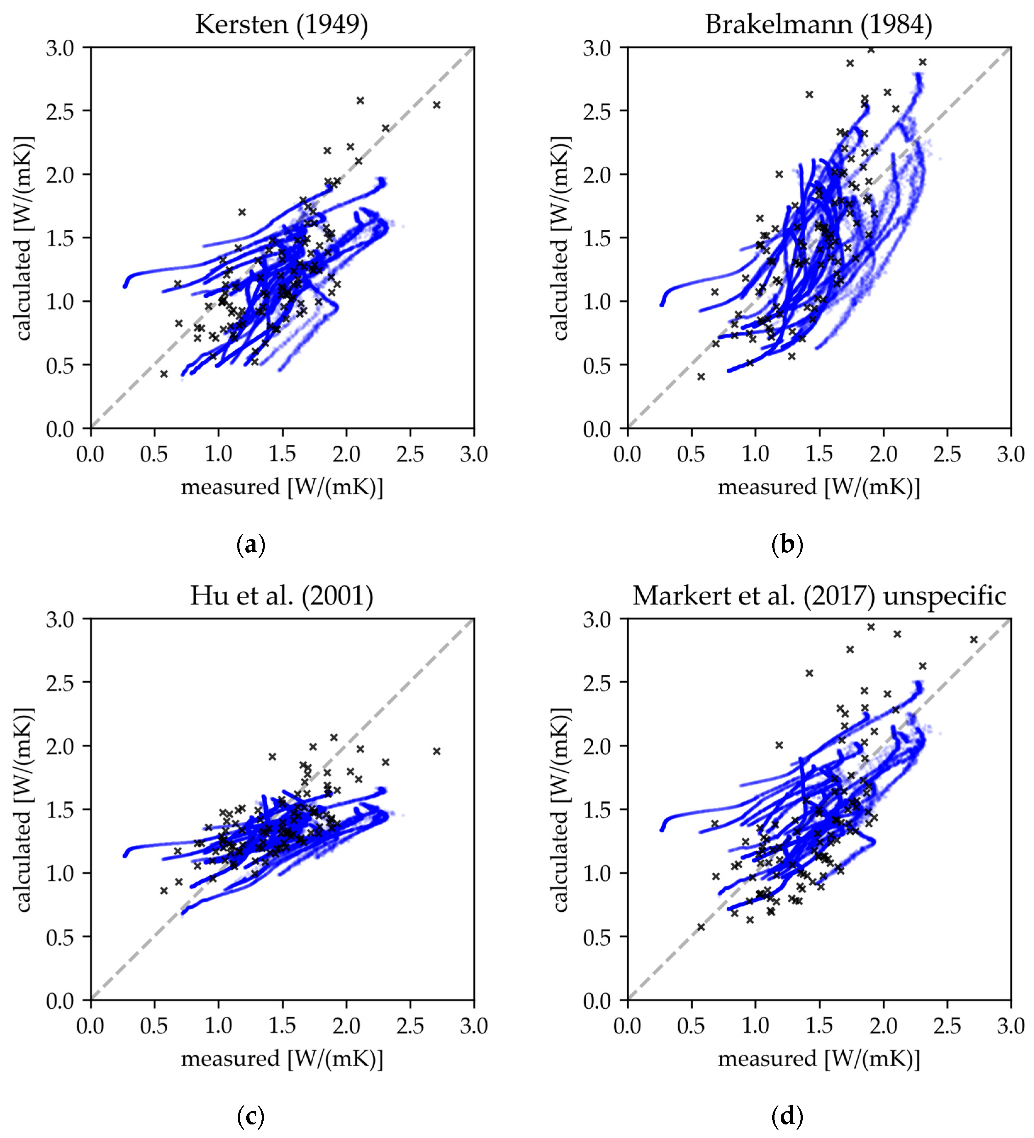
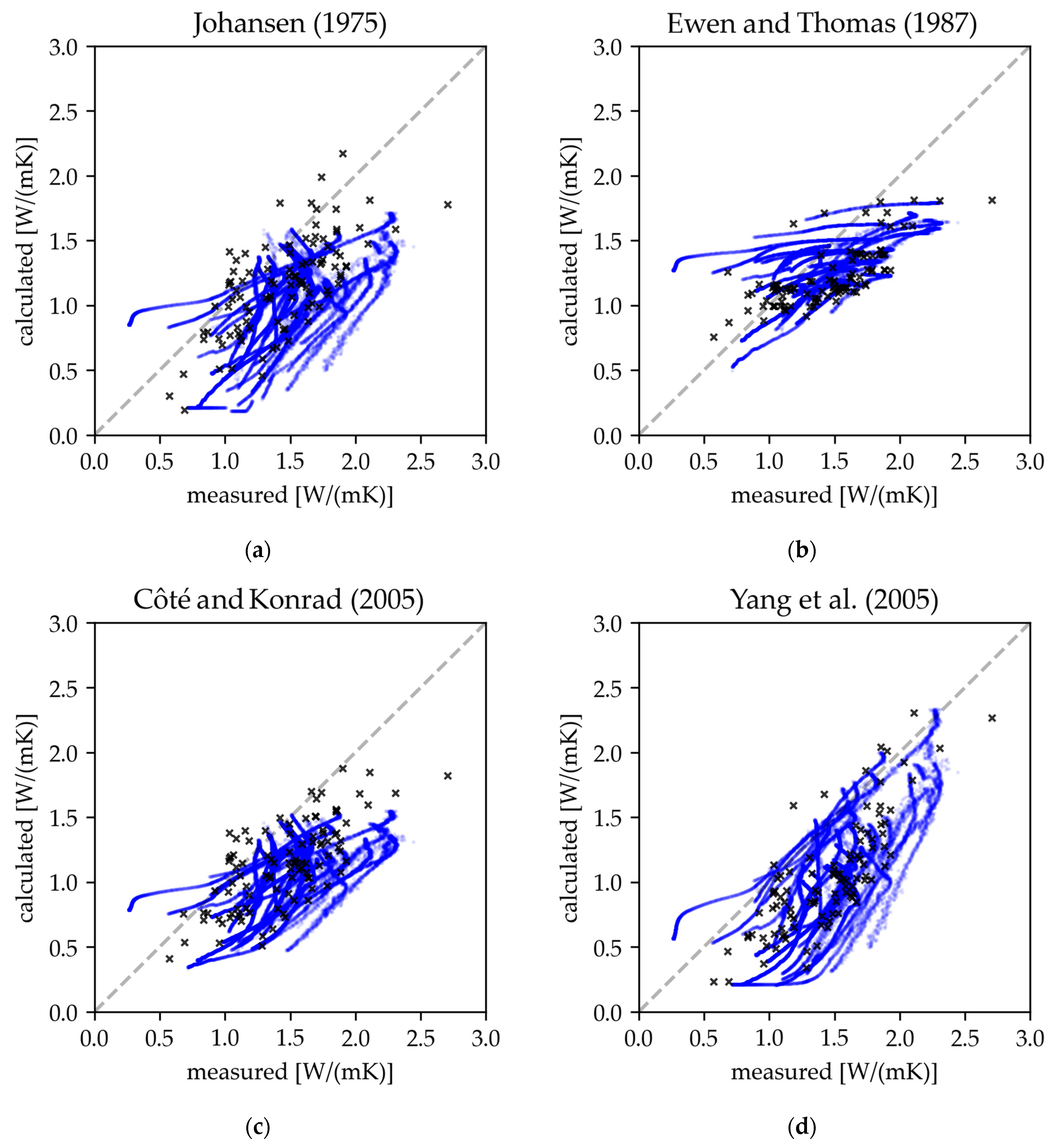
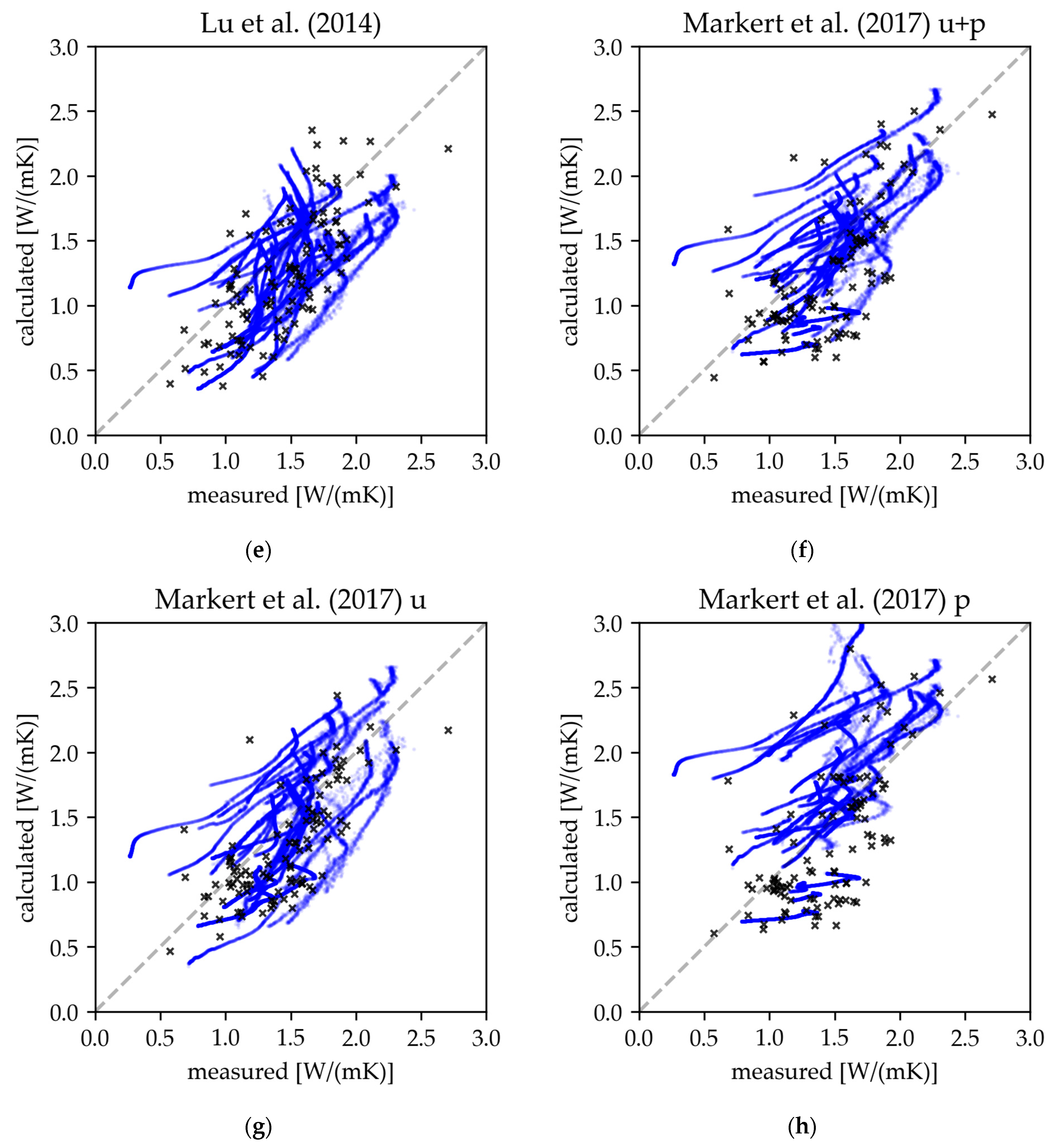
The results of the validation considering the entire set of measurement data are shown in

Table 10. Results of the validation in the form of the key indicator RMSE and bias considering the entire measurement dataset, with w ≥ 1% for sandy soils and w ≥ 7% for clay and silt soils, for all selected literature models.

Model		RMSE (W/(m∙K))	Bias
Kersten (1949)		0.37	−0.26
Johansen (1975)		0.45	−0.40
Brakelmann (1984)		0.35	−0.02
Ewen and Thomas (1987)		0.31	−0.16
Hu et al. (2001)		0.28	−0.10
Côté and Konrad (2005)		0.44	−0.38
Yang et al. (2005)		0.47	−0.45
Lu et al. (2014)		0.36	−0.17
Markert et al. (2017)	unspecific	0.29	−0.05
	u+p	0.32	−0.15
	u	0.31	−0.11
	p	0.40	0.00

and as scatter plots in Figure 3 and Figure A1.

Overall, RMSE values between 0.28 and 0.47 W/(m∙K) were determined. The bias values were almost exclusively in the negative range, meaning that the calculated thermal conductivity was underestimated, on average, by the literature models when compared to the measured values.

In the validation, the Hu et al. (2001) model, using only bulk density and water content-derived input parameters, showed the lowest RMSE value of 0.28 W/(m∙K), with an average underestimation of the thermal conductivity with a bias value of −0.10. The RMSE value for the Markert et al. (2017) model, here the texture group unspecific sub-model, was only marginally higher, with a value of 0.29 W/(m∙K). With a bias value of −0.05, the thermal conductivity was underestimated, to a minor extent. The texture group specific sub-models “u + p” and “u” also showed comparably low deviations from the measured values, with RMSE values of 0.31 and 0.32 W/(m∙K). Similarly, a low RMSE value of 0.31 W/(m∙K) was determined for the Ewen and Thomas (1987) model, again underestimating thermal conductivity, with a bias value of −0.16.

The Kersten (1949) model, for which the knowledge of the exact grain size distribution is not required for the calculation of the thermal conductivity, exhibits a higher error, with an RMSE value of 0.37 W/(m∙K) compared to the error rates of the models previously mentioned. However, the Johansen (1975) model, the Côté and Konrad (2005) model, and the Yang et al. (2005) model showed significantly higher deviations. With a bias value of −0.26, the Kersten (1949) model showed a significant underestimation of the thermal conductivity compared to the measured values.

3.2. Validation of the Models Considering Subsets in Terms of Soil Texture and Moisture

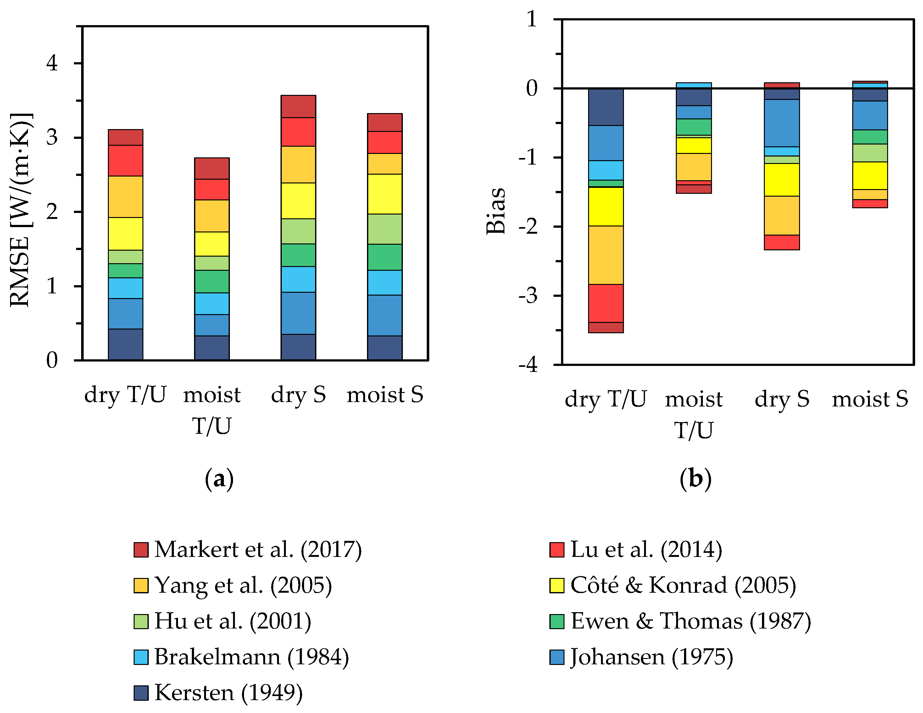
The results of the validations considering different subsets in terms of moisture content and soil texture are graphically shown in Figure 4 to express general patterns.

In general, but not for all models, the RMSE values appeared to be higher for sandy soils in comparison to silt and clay soils. Sandy soils generally have higher thermal conductivity than fine-grained soils. The quartz content, and possibly, the grain size of the sand content, can be decisively influencing variables on the thermal conductivity, which are only assumed or not considered in detail in the models studied here.

With the bias values, almost exclusively negative values, i.e., an underestimation of the thermal conductivity, were achieved. In general, higher negative values were shown for dry soil conditions. Particularly high bias amounts resulted for dry clay and silt soils. The partially significant negative bias values for dry soils, especially for silty and clay soils could be due to shrinking processes that may occur during the evaporation method, along with the resulting increase in bulk density, which further positively influence the measured thermal conductivity [18]. However, this correlation does not apply to all soil texture categories or models, including the Ewen and Thomas (1987) model, the Hu et al. (2001) model, and the Markert et al. (2017) model.

The RMSE and bias values for the individual models and subsets are listed in detail in

Table 11. RMSE values [W/(m∙K)] for the validation regarding the considered subsets in terms of soil texture and moisture for the selected literature models. The lowest RMSE values are marked in bold.

Model		Clay and Silt			Sand			Clay, Silt, and Sand
		Dry	Moist	All	Dry	Moist	All	Dry	Moist	All
Kersten (1949)		0.42	0.33	0.38	0.35	0.33	0.35	0.39	0.33	0.37
Johansen (1975)		0.41	0.29	0.36	0.57	0.55	0.58	0.48	0.40	0.45
Brakelmann (1984)		0.28	0.29	0.33	0.35	0.33	0.39	0.31	0.31	0.35
Ewen and Thomas (1987)		0.19	0.31	0.28	0.30	0.35	0.35	0.24	0.33	0.31
Hu et al. (2001)		0.18	0.19	0.20	0.34	0.41	0.38	0.25	0.28	0.28
Côté and Konrad (2005)		0.44	0.32	0.39	0.48	0.54	0.52	0.46	0.41	0.44
Yang et al. (2005)		0.56	0.43	0.51	0.50	0.28	0.42	0.53	0.37	0.47
Lu et al. (2014)		0.41	0.28	0.35	0.38	0.29	0.36	0.40	0.29	0.36
Markert et al. (2017)	unspecific	0.22	0.29	0.29	0.30	0.24	0.29	0.25	0.27	0.29
	u + p	0.29	0.35	0.35	0.31	0.23	0.28	0.30	0.30	0.32
	u	0.28	0.28	0.29	0.35	0.29	0.34	0.31	0.28	0.31
	p	0.27	0.43	0.39	0.48	0.34	0.41	0.36	0.39	0.40

and

Table 12. Bias values for the validation regarding the considered subsets in terms of soil texture and moisture for the selected literature models. The values that are closest to 0.00 are marked in bold.

Model		Clay and Silt			Sand			Clay, Silt and Sand
		Dry	Moist	All	Dry	Moist	All	Dry	Moist	All
Kersten (1949)		−0.53	−0.25	−0.33	−0.16	−0.18	−0.17	−0.36	−0.22	−0.26
Johansen (1975)		−0.51	−0.19	−0.30	−0.69	−0.42	−0.54	−0.59	−0.29	−0.40
Brakelmann (1984)		−0.28	0.08	−0.02	−0.13	0.08	−0.01	−0.21	0.08	−0.02
Ewen and Thomas (1987)		−0.10	−0.24	−0.20	0.00	−0.20	−0.11	−0.05	−0.22	−0.16
Hu et al. (2001)		−0.01	−0.04	−0.03	−0.11	−0.26	−0.19	−0.05	−0.13	−0.10
Côté and Konrad (2005)		−0.56	−0.23	−0.34	−0.47	−0.40	−0.44	−0.52	−0.30	−0.38
Yang et al. (2005)		−0.84	−0.39	−0.54	−0.56	−0.15	−0.32	−0.72	−0.29	−0.45
Lu et al. (2014)		−0.55	−0.06	−0.18	−0.21	−0.12	−0.16	−0.40	−0.09	−0.17
Markert et al. (2017)	unspecific	−0.15	−0.12	−0.12	0.08	0.03	0.05	−0.05	−0.06	−0.05
	u + p	−0.31	−0.31	−0.29	0.10	0.02	0.05	−0.13	−0.17	−0.15
	u	−0.28	−0.20	−0.22	0.05	0.06	0.05	−0.13	−0.09	−0.11
	p	−0.09	−0.17	−0.13	0.23	0.13	0.17	0.05	−0.04	0.00

.

For the Hu et al. (2001) model, a very low RMSE value of 0.20 W/(m∙K) was obtained for clayey and silty soils, largely independent of the saturation, with only a slight underestimation of λ, on average. For this soil texture category, moisture had almost no influence on the quality of the model. However, the deviations of the calculated thermal conductivities compared to the measured values were significantly higher for sandy soils, with an RMSE value of 0.38 W/(m∙K). The deviations were the highest for moist sandy soils, with an RMSE value of 0.41 W/(m∙K) and a bias value of −0.26.

The texture group unspecific Markert et al. (2017) model showed low RMSE values of 0.22 and 0.30 W/(m∙K), depending on the soil texture and moisture. The thermal conductivity for clay and silt soils was underestimated by a bias value of −0.12, on average. For sandy soils, the thermal conductivity was slightly overestimated compared to the measured values, with a bias value of 0.05. The “u + p” sub-model also showed similarly small deviations for sandy soils.

The Ewen and Thomas (1987) model showed differences between the validation results for dry and wet soil conditions. Low RMSE values of up to 0.19 and 0.30 W/(m∙K) were obtained for dry soils, whereby the thermal conductivity for clay and silt soils is underestimated by a bias value of 0.10, on average. No underestimation or overestimation was observed for dry sandy soils. For moist soils, higher RMSE values of 0.31 and 0.35 W/(m∙K) and a considerable underestimation, with bias values of −0.24 and −0.20, were achieved.

The Kersten (1949) model showed the highest deviation, with an RMSE value of 0.42 W/(m∙K) for dry clay and silt soils and a clear average underestimation of the thermal conductivity compared to the measured values, with a bias value of −0.53. The smallest deviations were found for moist soils, with an RMSE value of 0.33 W/(m∙K).

4. Discussion

For examples based on the Johansen (1975) model, the quartz content is required for the calculation of the thermal conductivity. In this study, the quartz content was assumed by deriving it from the sand content; thus, this parameter exhibits significant uncertainty. Changing the assumed quartz content, e.g., due to a different calculation equation, can lead to significantly different results [32]. Therefore, actual measurements of the thermal conductivity are always preferable. Especially in the case of specific mineralogical compositions or organic soils, high errors using empirical models are to be expected. For example, thermal conductivity measurements of decomposed basalt showed significantly lower values in comparison to those for loamy valley deposits, despite similar grain size distribution and bulk density [18]. This is mainly due to the low particle thermal conductivity of basalt [21].

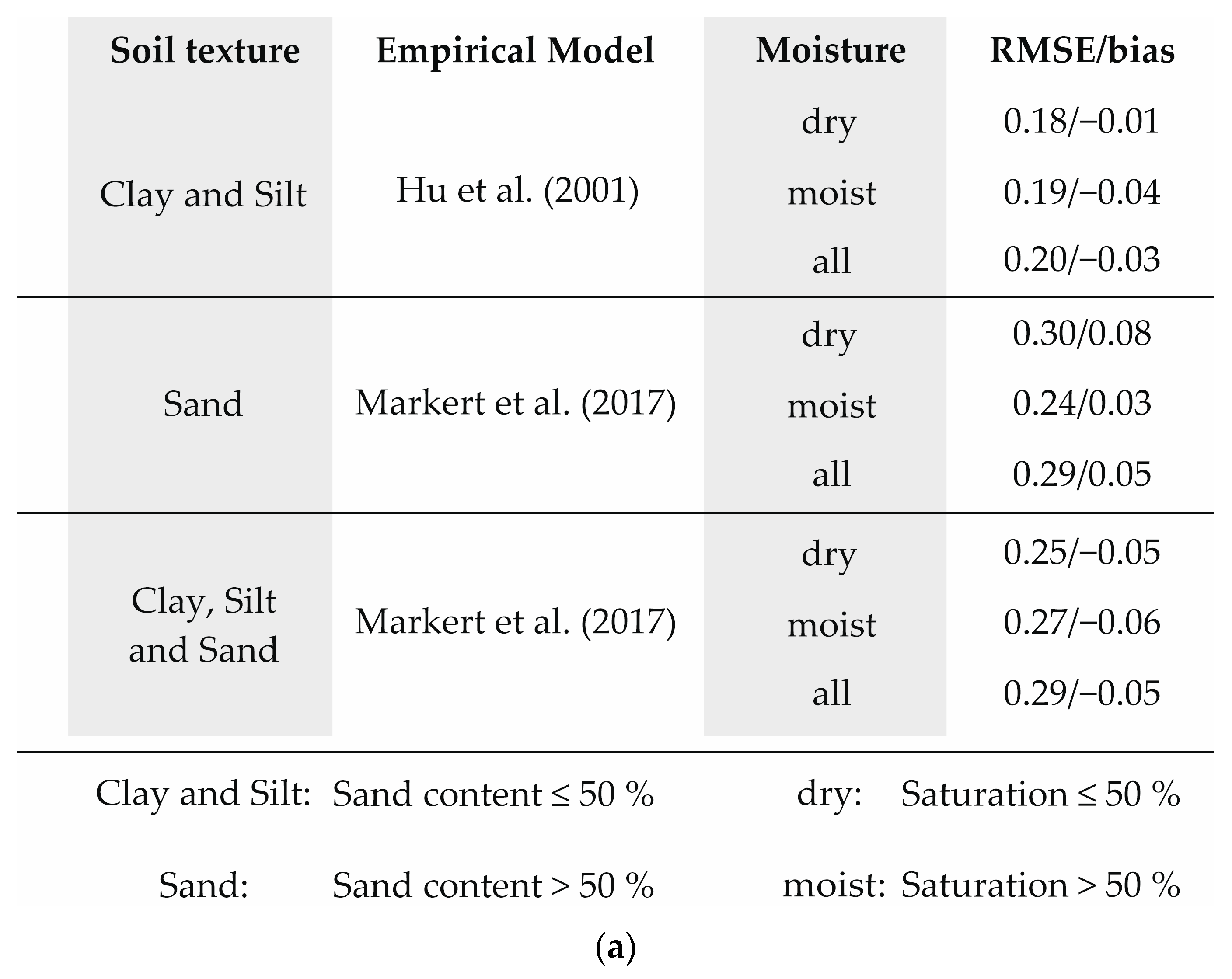
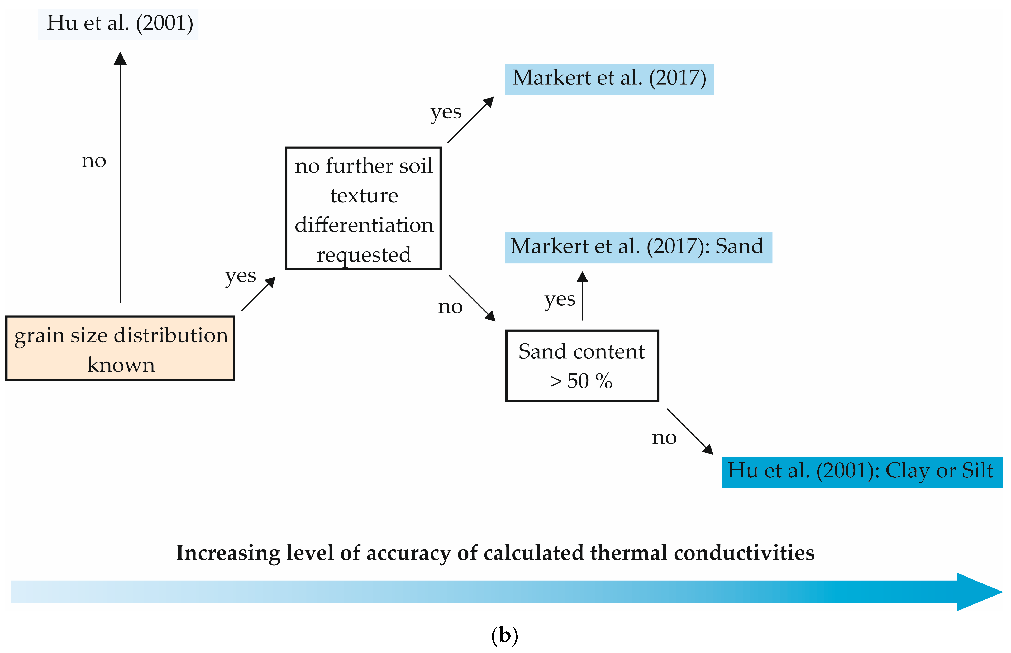
In addition to the validation of models for the calculation of the thermal conductivity of soils based on the parameters of bulk density, moisture content, and grain size distribution, the aim of the study was to develop a practical guideline for the use of empirical literature models, additionally based on the validation results of the considered subsets. For the development of the guideline, the determined RMSE and bias values of the validation of this study were used, as well as the results for the selected moisture and soil texture categories. The guideline is shown in Figure 5.

In this study, the Hu et al. (2017) model and the Markert et al. (2017) model (here: texture group unspecific sub-model) were identified as the generally best-fitting models. The guideline is based solely on the results of this study. The RMSE values for the Hu et al. (2001) model and for the Markert et al. (2017) model are almost identical for the soil texture- and moisture-independent approach. However, since the Hu et al. (2001) model shows significantly higher RMSE values for sandy soils, the Markert et al. (2017) model is proposed here, if information on grain size distribution is available. As can be seen in Figure 5a and Table 11, soil moisture is not a decisive factor for the selection of the literature model. The Ewen and Thomas (1987) model showed the lowest RMSE value for dry soils in general, which was, however, neglected here for reasons of simplicity. The results can therefore be broken down into a simple decision tree (Figure 5b). When using the Markert et al. (2017) model to calculate the thermal conductivity of sandy soils, as proposed here, the slight overestimation of the thermal conductivity by the model should be considered.

If the exact grain size distribution is not known, the Hu et al. (2017) model, with the approach and assumptions applied in this study, can be used to generate particularly high accuracy for clayey and silty soils. In the applied approach, only porosity and saturation are required as input parameters for the calculation of the thermal conductivity, while other parameters are assumed and not calculated, as in comparable models.

Furthermore, if the exact grain size distribution is not known, the Kersten (1949) model can be used to calculate the thermal conductivity, based on a rough estimate of the sand content (≤50% or >50%) and using a knowledge of the bulk density and water content, with no further assumptions. This simplicity enables the Kersten (1949) model to be used for preliminary thermal exploration, e.g., for derivation of thermal conductivity from geoelectric field measurements [18,43]. The validation of this study showed an RMSE value of 0.37 W/(m∙K). This significant underestimation would provide a large degree of certainty regarding the estimation of thermal conductivity for the dimensioning and design of thermal infrastructure projects.

For the sake of completeness, however, the results of other validation studies should also be briefly mentioned. In the study by He et al. [32], the models of Johansen [35,36], Côté and Konrad [21], Côté and Konrad [44], Lu et al. [45], Tarnawski et al. [46], and Yan et al. [47] were determined to be the best-fitting models without free parameters. In addition to the model of Markle et al. [28], which, however, requires a fitting parameter, Wessolek et al. [34] also found the Hu et al. (2001) model to be the model with the lowest RMSE value. However, the Markert et al. (2017) model was not included in both studies.

5. Conclusions

By validating selected empirical models for calculating the thermal conductivity of unconsolidated soils using 59 series of measurements, it was possible to derive a practicable guideline in the form of a decision tree for the use of thermal conductivity models considering different soil texture categories. This is based on knowledge of the physical soil parameters of moisture content, bulk density, and if applicable, grain size distribution.

The measurement series each consist of a different number of measurement points. However, each measurement series received equal consideration for validation. The measurements were carried out on soil samples with a known grain size distribution, bulk density, and moisture content using single-needle sensors. As the measurement series originate from various research projects in Germany, a wide range of soil texture classes was included.

The correspondence between the calculated thermal conductivities and the measured values was evaluated using the RMSE and the bias value. As a result, it was determined that the thermal conductivity is mainly underestimated by the literature models, on average, with basically higher deviations for sandy soils. The Hu et al. (2001) model, which is based on the Johansen (1975) model, and the Markert et al. (2017) model were identified as the best-fitting models. The Hu et al. (2001) model showed particularly low RMSE values for clay and silty soils, while for sandy soils, the Markert et al. (2017) model showed the lowest deviations. The Hu et al. (2001) model, with the approach and assumptions used in this study, can also be employed to calculate thermal conductivity when grain size distribution information is not available.

If the exact grain size distribution is not known, the Kersten (1949) model can also be used by roughly estimating the sand content. Although this model shows higher deviations, the significant underestimation of the thermal conductivity on average provides a large degree of certainty for the planning of thermal infrastructure projects.

As the soil samples were obtained exclusively from Germany, the applicability of the results or the guideline on a global scale is limited. Future research could therefore extend the validation carried out to international soil samples. In addition, the guideline could be extended by the integration of further models or by additional subset analyses, e.g., with regard to organic matter content or bulk density.

Due to the small number of input parameters and the high accuracy of the Hu et al. (2001) model, future attempts could also be made to perform thermal exploration using geoelectric field measurements by deriving thermal conductivities using this model.

References

- Papadis, E.; Tsatsaronis, G. Challenges in the decarbonization of the energy sector. Energy 2020, 205, 118025. [Google Scholar] [CrossRef]
- Schwarz, H.; Jocic, N.; Bertermann, D. Development of a Calculation Concept for Mapping Specific Heat Extraction for Very Shallow Geothermal Systems. Sustainability 2022, 14, 4199. [Google Scholar] [CrossRef]
- Bertermann, D.; Klug, H.; Morper-Busch, L.; Bialas, C. Modelling vSGPs (very shallow geothermal potentials) in selected CSAs (case study areas). Energy 2014, 71, 226–244. [Google Scholar] [CrossRef]
- Ohlsen, B.; Horzella, J.; Bock, T.; Lucki, P.; Bertermann, D.; Wagner, J.; Grunewald, J.; Petzold, H.; Mueller, D.; Schreiber, T.; et al. Abschlussbericht ErdEis II—Erdeisspeicher und Oberflächennaheste Geothermie; Energie Plus Concept GmbH: Nürnberg, Germany, 2023. [Google Scholar]
- Zeh, R.; Ohlsen, B.; Philipp, D.; Bertermann, D.; Kotz, T.; Jocic, N.; Stockinger, V. Large-Scale Geothermal Collector Systems for 5th Generation District Heating and Cooling Networks. Sustainability 2021, 13, 6035. [Google Scholar] [CrossRef]
- Boesten, S.; Ivens, W.; Dekker, S.C.; Eijdems, H. 5th generation district heating and cooling systems as a solution for renewable urban thermal energy supply. Adv. Geosci. 2019, 49, 129–136. [Google Scholar] [CrossRef]
- Buffa, S.; Cozzini, M.; D’Antoni, M.; Baratieri, M.; Fedrizzi, R. 5th generation district heating and cooling systems: A review of existing cases in Europe. Renew. Sustain. Energy Rev. 2019, 104, 504–522. [Google Scholar] [CrossRef]
- García-Céspedes, J.; Herms, I.; Arnó, G.; de Felipe, J. Fifth-Generation District Heating and Cooling Networks Based on Shallow Geothermal Energy: A review and Possible Solutions for Mediterranean Europe. Energies 2022, 16, 147. [Google Scholar] [CrossRef]
- Bertermann, D.; Drefke, C.; Stegner, J.; Wessolek, G. Interaktionen des Erdkabelsystems SuedLink mit der Kabelumgebung, Bodenkundlich-Technische Aspekte; FAU University Press: Erlangen, Germany, 2020; p. 96. [Google Scholar]
- Brakelmann, H. Physical Principles and Calculation Methods of Moisture and Heat Transfer in Cable Trenches; VDE Verlag: Berlin, Germany, 1984; p. 93. [Google Scholar]
- Kroener, E.; Vallati, A.; Bittelli, M. Numerical simulation of coupled heat, liquid water and water vapor in soils for heat dissipation of underground electrical power cables. Appl. Therm. Eng. 2014, 70, 510–523. [Google Scholar] [CrossRef]
- Abu-Hamdeh, N.H. Thermal Properties of Soils as affected by Density and Water Content. Biosyst. Eng. 2003, 86, 97–102. [Google Scholar] [CrossRef]
- Abu-Hamdeh, N.H.; Reeder, R.C. Soil Thermal Conductivity Effects of Density, Moisture, Salt Concentration, and Organic Matter. Soil Sci. Soc. Am. J. 2000, 64, 1285–1290. [Google Scholar] [CrossRef]
- Farouki, O.T. Thermal Properties of Soils; Cold Regions Research and Engineering Lab: Hanover, NH, USA, 1981. [Google Scholar]
- Barry-Macaulay, D.; Bouazza, A.; Singh, R.M.; Wang, B.; Ranjith, P.G. Thermal conductivity of soils and rocks from the Melbourne (Australia) region. Eng. Geol. 2013, 164, 131–138. [Google Scholar] [CrossRef]
- He, H.; Dyck, M.F.; Horton, R.; Ren, T.; Bristow, K.L.; Lv, J.; Si, B. Development and Application of the Heat Pulse Method for Soil Physical Measurements. Rev. Geophys. 2018, 56, 567–620. [Google Scholar] [CrossRef]
- Low, J.E.; Loveridge, F.A.; Powrie, W.; Nicholson, D. A comparison of laboratory and in situ methods to determine soil thermal conductivity for energy foundations and other ground heat exchanger applications. Acta Geotech. 2015, 10, 209–218. [Google Scholar] [CrossRef]
- Rammler, M.; Schwarz, H.; Wagner, J.; Bertermann, D. Comparison of Measured and Derived Thermal Conductivities in the Unsaturated Soil Zone of a Large-Scale Geothermal Collector System (LSC). Energies 2023, 16, 1195. [Google Scholar] [CrossRef]
- Schjønning, P. Thermal conductivity of undisturbed soil—Measurements and predictions. Geoderma 2021, 402, 115188. [Google Scholar] [CrossRef]
- Markert, A.; Peters, A.; Wessolek, G. Analysis of the Evaporation Method to Obtain Soil Thermal Conductivity Data in the Full Moisture Range. Soil Sci. Soc. Am. J. 2016, 80, 275–283. [Google Scholar] [CrossRef]
- Côté, J.; Konrad, J.-M. A generalized thermal conductivity model for soils and construction materials. Can. Geotech. J. 2005, 42, 443–458. [Google Scholar] [CrossRef]
- De Vries, D.A. Thermal properties of soils. In Physics of Plant Environment; North-Holland Publishing Co.: Amsterdam, The Netherlands, 1963; pp. 210–235. [Google Scholar]
- Ewen, J.; Thomas, H.R. The thermal probe—A new method and its use on an unsaturated sand. Geotechnique 1987, 37, 91–105. [Google Scholar] [CrossRef]
- Hu, X.-J.; Du, J.-H.; Lei, S.-Y.; Wang, B.-X. A model for the thermal conductivity of unconsolidated porous media based on capillary pressure-saturation relation. Int. J. Heat Mass Transf. 2001, 44, 247–251. [Google Scholar] [CrossRef]
- Kersten, M. Thermal Properties of Soils; University of Minnesota: Mineapolis, MN, USA, 1949. [Google Scholar]
- Lu, Y.; Lu, S.; Horton, R.; Ren, T. An Empirical Model for Estimating Soil Thermal Conductivity from Texture, Water Content, and Bulk Density. Soil Sci. Soc. Am. J. 2014, 78, 1859–1868. [Google Scholar] [CrossRef]
- Markert, A.; Bohne, K.; Facklam, M.; Wessolek, G. Pedotransfer Functions of Soil Thermal Conductivity for the Textural Classes Sand, Silt, and Loam. Soil Sci. Soc. Am. J. 2017, 81, 1315–1327. [Google Scholar] [CrossRef]
- Markle, J.M.; Schincariol, R.A.; Sass, J.H.; Molson, J.W. Characterizing the Two-Dimensional Thermal Conductivity Distribution in a Sand and Gravel Aquifer. Soil Sci. Soc. Am. J. 2006, 70, 1281–1294. [Google Scholar] [CrossRef]
- Sadeghi, M.; Ghanbarian, B.; Horton, R. Derivation of an Explicit Form of the Percolation-Based Effective-Medium Approximation for Thermal Conductivity of Partially Saturated Soils. Water Resour. Res. 2018, 54, 1389–1399. [Google Scholar] [CrossRef]
- Yang, K.; Koike, T.; Ye, B.; Bastidas, L. Inverse analysis of the role of soil vertical heterogeneity in controlling surface soil state and energy partition. J. Geophys. Res. 2005, 11, 1–15. [Google Scholar] [CrossRef]
- Dong, Y.; McCartney, J.S.; Lu, N. Critical Review of Thermal Conductivity Models for Unsaturated Soils. Geotech. Geol. Eng. 2015, 33, 207–221. [Google Scholar] [CrossRef]
- He, H.; Noborio, K.; Johansen, Ø.; Dyck, M.F.; Lv, J. Normalized concept for modelling effective soil thermal conductivity from dryness to saturation. Eur. J. Soil Sci. 2019, 71, 27–43. [Google Scholar] [CrossRef]
- Tarnawski, V.R.; McCombie, M.L.; Leong, W.H.; Coppa, P.; Corasaniti, S.; Bovesecchi, G. Canadian Field Soils IV: Modeling Thermal Conductivity at Dryness and Saturation. Int. J. Thermophys. 2018, 39, 35. [Google Scholar] [CrossRef]
- Wessolek, G.; Bohne, K.; Trinks, S. Validation of Soil Thermal Conductivity Models. Int. J. Thermophys. 2022, 44, 20. [Google Scholar] [CrossRef]
- Johansen, O. Thermal Conductivity of Soils; Cold Regions Research and Engineering Lab: Hanover, NH, USA, 1977. [Google Scholar]
- Johansen, O. Varmeledningsevne av Jordarter. Ph.D. Thesis, University of Trondheim, Trondheim, Norway, 1975. [Google Scholar]
- IEEE Std 442-1981; IEEE Guide for Soil Thermal Resistivity Measurements. IEEE Power Engineering Society: New York, NY, USA, 1981.
- ASTM D5334; Standard Test Method for Determination of Thermal Conductivity of Soil and Soft Rock by Thermal Needle Probe Procedure. ASTM International: West Conshohocken, PA, USA, 2014.
- Ardiansyah; Shiozawa, S.; Nishida, K. Thermal properties and shrinkage-swelling characteristic of clay soil in a tropical paddy field. J. Jpn. Soc. Soil Phys. 2008, 110, 67–77. [Google Scholar] [CrossRef]
- DIN EN ISO 14688-1; Geotechnical Investigation and Testing—Identification and Classification of Soil—Part 1: Identification and Description (ISO 14688-1:2017). German version EN ISO 14688-1:2018. Beuth Verlag GmbH: Berlin, Germany, 2020.
- Hu, G.; Zhao, L.; Wu, X.; Li, R.; Wu, T.; Xie, C.; Pang, Q.; Zou, D. Comparison of the thermal conductivity parameterizations for a freeze-thaw algorithm with a multi-layered soil in permafrost regions. Catena 2017, 156, 244–251. [Google Scholar] [CrossRef]
- Peters-Lidard, C.D.; Blackburn, E.; Liang, X.; Wood, E.F. The Effect of Soil Thermal Conductivity Parameterization on Surface Energy Fluxes and Temperatures. J. Atmos. Sci. 1998, 55, 1209–1224. [Google Scholar] [CrossRef]
- Bertermann, D.; Schwarz, H. Laboratory device to analyse the impact of soil properties on electrical and thermal conductivity. Int. Agrophys. 2017, 31, 157–166. [Google Scholar] [CrossRef]
- Côté, J.; Konrad, J.-M. Estimating Thermal Conductivity of Pavement Granular Materials and Subgrade Soils. Transp. Res. Rec. J. Transp. Res. Board 2006, 1967, 10–19. [Google Scholar] [CrossRef]
- Lu, S.; Ren, T.; Gong, Y.; Horton, R. An Improved Model for Predicting Soil Thermal Conductivity from Water Content at Room Temperature. Soil Sci. Soc. Am. J. 2007, 71, 8–14. [Google Scholar] [CrossRef]
- Tarnawski, V.R.; Momose, T.; Leong, W.H. Assessing the impact of quartz content on the prediction of soil thermal conductivity. Geotechnique 2009, 59, 331–338. [Google Scholar] [CrossRef]
- Yan, H.; He, H.; Dyck, M.; Jin, H.; Li, M.; Si, B.; Lv, J. A generalized model for estimating effective soil thermal conductivity based on the Kasubuchi algorithm. Geoderma 2019, 353, 227–242. [Google Scholar] [CrossRef]
Figure 1.
Schematic illustration of the (a) evaporation method and (b) the punctual method of thermal conductivity measurement used for validation, taken from the work of Rammler et al. [18], with ω1/2 = medium water contents, ωdry = water content after oven drying, and ωsat = water content after capillary saturation. Also shown are three exemplary measurement series, which are distinguished by their different colors, for measurements (c) with the punctual method, (d) evaporation method with temporary measurements, and (e) evaporation method with continuous measurements (measuring points cannot be recognized as points due to the high data density).
Figure 2.
Grain size distributions and soil texture classes according to USDA soil classifications. Grain size limits were determined according to the grain size limits of the DIN EN ISO 14688-1 [40] or USDA soil classification. The deviations at the silt–sand boundary at 0.063 mm, according to DIN EN ISO 14688-1, and at 0.05 mm, according to USDA soil classification, were neglected here. The red line illustrates the boundary of >50% and <50% sand content (fSand). Different measurement series can have the same grain size distribution. If present, particles coarser than 2 mm were sieved out before the measurements. For two soil samples with a sand content ≥ 93%, the remaining fine-grained content was assumed to be half clay and half silt.
Figure 3.
Results of the validation as exemplary scatter plots for the models of (a) Kersten [25], (b) Brakelmann [10], (c) Hu et al. [24] and (d) Markert et al. [27] (here: texture group independent sub-model) considering the entire measurement data, with w ≥ 1% for sandy soils and w ≥ 7% for clay and silt soils. Measurement points of measurement series with a high data density (98 to 1882 measurement points per measurement series) are shown as blue dots. Measurement points from measurement series with low data density (3 to 10 measurement points per measurement series) are shown as black crosses.
Figure 4.
Bar charts of (a) RMSE and (b) bias values for the considered subsets in terms of soil texture and moisture for all selected models [10,21,23,24,25,26,27,30,35,36]. As a representative of the Markert et al. (2017) models, only the “unspecific” texture group sub-model was considered.
Figure 5.
(a) Basis of evaluation for the guideline derived from the results of the validation for the use of empirical literature models to calculate the thermal conductivity of unconsolidated soils (b) and the guideline in form of a decision tree. The basis for this is the knowledge (or assumption) of the bulk density and moisture content of the soil. The RMSE and bias values (RMSE in W/(m∙K)/bias) are indicated in each case to assess the quality of the model. For sandy soils, the texture group independent sub-model, or the “u + p” sub-model of Markert et al. [27], can be used. In the figure, RMSE and bias values are shown for the texture group unspecific sub-model. Negative bias values correspond to an average underestimation of the thermal conductivity by the model. The validation was carried out for the range, with a gravimetric water content ≥ 1% for sandy soils and ≥7% for clay and silty soils. The calculation of the thermal conductivity with unknown grain size distribution, using the model of Hu et al. [24], is considered to be less accurate here due to the higher RMSE values for the sandy soils compared to those of the approach by Markert et al. [27].