
Soil and Land Cover Interrelationships: An Analysis Based on the Jenny’s Equation


1
Department of Environment, Centro de Investigaciones Energéticas, Medioambientales y Tecnológicas (CIEMAT), Avenida Complutense, 40, 28040 Madrid, Spain
2
Department of Geology and Geochemistry, Faculty of Science, Autonomous University of Madrid, Campus de Cantoblanco, Calle Francisco Tomás y Valiente 7, 28049 Madrid, Spain
3
Departamento de Física de la Tierra y Astrofísica, Universidad Complutense de Madrid (UCM), Plaza de Ciencias, 1, Ciudad Universitaria, 28040 Madrid, Spain
*
Author to whom correspondence should be addressed.
Soil Syst. 2023, 7(2), 31; https://doi.org/10.3390/soilsystems7020031
Submission received: 24 October 2022
/
Revised: 2 March 2023
/
Accepted: 28 March 2023
/
Published: 5 April 2023
Abstract
:This research analyzes the relationships between “soil” and “organisms” within the framework of the Jenny equation, a fundamental expression in soil science that is the theoretical basis for modeling the complex occurrence of soils on landscapes. This analysis is based on the interpretation of the indeterminate function “f” of the equation as “statistical dependence between categorical variables”. The categories of the “soil” component of the equation have been defined as “diagnostic horizons”, and those of the “organisms” factor as synthetic types of “land cover”. After applying these criteria to 424 soil profiles studied in a region with an oceanic climate in northern Spain, a multiple correspondence analysis showed pedologically consistent groupings between diagnostic horizons and categories of climate, land cover, relief, and parent material factors. Subsequently, a bivariate analysis detailed pedologically consistent relationships between diagnostic horizons and land cover categories. In the context the scarcity of quantitative information on soil and forming factor relationships, this work provides criteria to statistically assess the role of land cover in such relationships. This soil forming factor is the one whose spatial representation is more generalized and detailed, hence its interest in the development of soil mapping models.
1. Introduction
The first expression relating to soil formation, “S = f(c,o,p)t”, was formulated by Dokuchaev in 1899; the term “S” refers to the soil, which is a mere function of the factors “c” (climate), “o” (organisms), and “p” (parent material) that interact over time (t) and determine its genesis [1]. This expression, and Jenny’s [2] subsequent formalization of environmental components as “parameters that define the state of the soil system” [3], requires for any kind of resolution that the indeterminate function “f” be replaced by some kind of “quantitative relationship” [4]. In any case, Jenny’s equation (S = f (cl, o, r, p, t …), where “cl” is (climate), “o” (organisms), “r” relief, “p” (parent material), and “t” (time) factors), provides a basis for the interpretation of soil attributes (physicochemically, morphologically, or taxonomically expressed) in terms of the factors associated with their genesis [5].
A clear separation between forming factors in such a way that one of them can be considered a constant while the others behave as independent variables is only theoretical; for example, soil evolution itself favors the development of plant cover, thus tending to co-evolve [6]. The contributions of organic matter determine the development of the soil by means of biochemical processes of weathering, humification, and cheluviation [7]; Similarly, the root system increases the susceptibility of the parent material to weathering [8]. Topography, together with the vegetation cover itself, determines the runoff-infiltration relationships, thus influencing soil moisture conditions [9]. Soil, climate, and vegetation are considered a coupled system: the climate affects soils and vegetation independently, while soil and vegetation interact with each other. However, some factors can, under certain conditions, exert a particularly strong influence on pedogenesis [10]. Vegetation is considered an “active forming factor” [11], a variable capable of exerting certain climate-independent effects [12], so that different vegetation cover types can determine different soil attributes in the homogeneity of other factors. This links to the concept of biofunctions [13,14]. It is important to highlight that this mutual association takes place between plant biomass and soil as “natural bodies”, and not so much between specific attributes of the vegetation cover and a selection of individual soil properties [15].
With the aim of establishing “quantitative relationships” between soils and soil-forming factors, the problem that arises is how to define such factors precisely enough for their statistical treatment. Organism factors, for example, cannot be feasibly treated as parametric variables [9]. Jenny [14] defined the “organisms” factor specifically in terms of vegetation, considering that it would have to be represented as “the vegetation currently existing in the place under study”. This was assumed, for the purposes of this work, for the concept of “land cover” [16]. Land cover is an easily recognizable factor through fieldwork and/or remote sensing techniques [17], which would facilitate establishing precise relationships between soils and formation factors to develop models to explain soil-landscape relationships, allowing soil mapping with greater precision and decreasing costs [9].
Likewise, any development of the Jenny equation (also called the “clorpt equation”) requires an equivalent definition of the “soil” component. In this sense, it is possible to consider soil taxa at different hierarchical levels as suitable candidates to represent such a component. Soil taxa synthesize in their own definition a large amount of pedological information and are widely represented worldwide in countless soil maps and studies; however, the soil classification systems used worldwide, WRBSR-FAO [18] and Soil Taxonomy [19], show different criteria to define and name the soil taxa, or “soil taxonomic units”. In this way, complex homogenization tasks are necessary when managing pedological information from soil maps or studies based on different classification systems. However, both WRBSR and soil taxonomy rely on the concept of “diagnostic horizons” [18,19], whose definitions are largely compatible in many cases between both systems. Each diagnostic horizon is synthetically defined by groups of quantitative, morphological, and physicochemical parameters. Similar to taxa, diagnostic horizons can be spatially represented to pedologically describe a region, and according to Bockheim [20], even more consistently than the cartography of high hierarchical levels such as suborders or great groups. In this sense, this research raises the possibility of assimilating the concept of diagnostic horizons to a simplified form of the “soil” component of the Jenny equation [21]. In addition to this compatibility between both systems, the limited number of diagnostic horizons must be considered in the face of a potentially unlimited number of statistical test. This represents a practical advantage, particularly when applying statistical tools to pedologically analyze a specific territory.
This study hypothesizes that the function “f” of the “clorpt” equation can be understood as “statistical dependence between variables”. In this regard, “diagnostic horizons”, understood as “categories of the soil variable”, are expected to show statistical dependency relationships with the “organisms” factor, understood as “categories of a land cover variable”. Specifically, it can also be hypothesized that the land cover factor contributes to explaining the variance of the surface horizons to a greater extent than that of the subsurface ones. For the development of both hypotheses, a study region characterized by a high variety of climate conditions, land covers, landforms, parent materials, and consequently, soils, has been selected. Information on this set of factors comes from an extensive soil survey previously carried out in the region. The specific objectives of this research require the development of (i) a methodology that allows transforming both “soil” and “soil forming factors” as components of the “clorpt” equation into categorical variables, (ii) to assess the influence of climate, organisms, relief, and parent material forming factors in the prevalence of specific diagnostic horizons by means of a multivariate analysis, and (iii) to specifically assess dependency relationships between land cover categories and soil diagnostic horizons.
The soil horizons and forming factor dependency relationships assessed in the study area are intended to provide objective criteria on the environmental factors associated with the presence or absence of certain diagnostic horizons. In particular, the relationships between diagnostic horizons and land cover were considered of special interest in the advances towards the spatial representation of natural soils, due to the generalization and high reliability of the information obtained on land cover, both by direct methods and by means of remote sensors.
2. Materials and Methods
2.1. Study Area: Summary of Soil Forming Factors
The geographical scope of this study is the Principality of Asturias, in northern Spain, in the context of a temperate-humid climate, whose physiographic characteristics determine a wide variety of soils and land cover types. This region comprises a physiographically complex territory with high lithological and geomorphological diversity. Altitudes range from sea level to above 2000 m; therefore, steep slopes prevail [21].
The climate is characterized by mild temperatures and regular and high average rainfall, ranging annually from 900 to 1800 mm [22], with notable differences mainly depending on altitude and exposure. Such conditions allow biological activity during most of the year, except at the highest altitudes. Certain local conditions associated with lithological and geomorphological factors lead to variations in this general scheme (acidity, rockiness, salinity, granulometry), as well as local drainage (excessive in rocky and/or steeper areas; deficient in depressions) or micro- or meso-climatic features (valleys with a rain-shadow effect and slopes exposed to windward).
2.2. Sampling Points: Soil Profiles and on-Ground Information on Soil Forming Factors
A soil survey was conducted in various field campaigns carried out in the years 2007, 2010, 2011, and 2012 with the participation of the corresponding author of this research. Various additional field tasks were carried out occasionally until 2017, covering a total of 424 sampling points [21], as shown in Figure 1. In each of them, a soil profile and the physiographic characteristics of its immediate surroundings were described. The survey of soil profiles was carried out with the criteria established by Schoeneberger et al. [23], which allowed obtaining systematic and organized information on relief, organisms, and parent material; on the other hand, factors such as altitude are key in the evaluation of the climatic conditions of each sampling point. The wide distribution of these points along the study area allows for a large part of the diversity of climate, land covers, landforms, and lithologies of the territory under study to be covered. Whenever possible, soil profiles were prepared in soil pits made with machinery, unless the conditions of the place (as frequently happened in such steep territory) did not allow access. In that case, sufficiently deep cuts in the ground along roads, paths, and other excavations were also used [24].
The classification of the soil profiles was carried out according to the Soil Taxonomy classification system [19]. From the point of view of the diagnostic horizons established by soil taxonomy, the ochric epipedon is dominant in the study area, with 54% of the soil profiles. Umbric (31%) and Mollic (15%) epipedons characterize the rest of the profiles. On the other hand, 55% of the profiles lack a subsurface diagnostic horizon, which highlights the importance of the soils that show limitations to soil development in this territory. The Cambic subsurface horizon is notably the most widespread; it is present in a third of the soil profiles (32%); that is, 73% of the profiles that show some development of subsurface horizons present such a horizon. Cambic horizons, together with the relative importance of the Umbric and Mollic epipedons, define the studied territory within the domain of the Inceptisols order as characteristic of temperate regions worldwide [25]. Regarding soils with higher degrees of evolution, argillic horizons are present in 21% of the soil profiles (Alfisols and Ultisols Orders), while Spodic horizons have only local importance (Spodosols Order) and are present in 6% of them.
The spatial distribution of the sampling points is presented below (Figure 1).
2.3. Statistical Analyses: Definition of the Components of the Clorpt Equation
Throughout this section, a methodology was developed aimed at compartmentalizing both “soil” and “soil forming factors” into variables and categories suitable for a statistical analysis. The variables established to define climate, organisms, relief, and parent material are those based on observable physiographical criteria at the location of each one of the 424 soil profiles and whose importance in pedogenesis is sufficiently proven in the literature. Given that the soil-forming factors are remarkably heterogeneous in terms of the parameters that characterize them (quantitative in some cases, nominally qualitative in others), it is necessary to compartmentalize such factors in order to obtain statistically treatable categorical variables. In general, the establishment of categories has been carried out with the aim of minimizing their total number.
For the purposes of this work, the time factor has not been considered, given the impossibility of cartographic representation except in specific situations such as certain chronosequences, that is, genetically related soils that evolved under similar conditions of vegetation, topography, and climate [26]. On most surfaces, only relative dating between contiguous landforms is possible, which limits the introduction of a quantifiable time factor similarly to the rest of forming factors [20].
Regarding land cover types, field observations were categorized according to the CORINE land cover inventory [27], although several modifications were considered for a better adaptation of the inventory to the characteristics of the territory under study. Finally, for the purposes of this work, eight categories derived from six CORINE land covers were established, as summarized in Table 1.
In the case of climate, since there is no direct data available on the climatic conditions of each soil profile location, it is necessary to establish relationships between climatic variables registered in meteorological stations (basically, precipitation and temperature) and the factors that can be measured in the location of the soil profile. Among the physiographic factors analyzed, altitude is the one that is mostly associated with precipitation and, especially, average annual temperature; linear regression models for precipitation and temperature vs. altitude showed R-squared values of 0.21 and 0.84, respectively [21]. Regarding rainfall, the regression model fits observed data in a very variable way when analyzing some specific river basins, obtaining r-square values ranging between 0.09 and 0.64. The influence of factors such as the rain shadow effect is significant in this territory, although its precise definition for the purposes of assigning a given sampling point is particularly complex [21]. Significance coefficients greater than 0.9 have been obtained by correlating the elevation of the Asturian weather stations with a digital elevation model (ASTER GDEM), with respect to official precipitation and temperature data [32]. The “distance to sea” factor has also been considered to be linearly modeled with rainfall and temperature; the values of the significance coefficient are 0.01 and 0.11, respectively. For the purposes of simplification, in this analysis, altitude was selected as a variable associated with the climatic factor. Five altitude categories have been considered for a range between 1 and 1957 m a.s.l.
Regarding the relief factor, three variables related to the geometry of the slope have been evaluated for their role in the development of erosion and deposition processes, keys in pedogenesis: slope value, slope shape, and relative position of the soil profile. These parameters were estimated in the field and corrected by digital cartography at 1:5000 (available at: https://ideas.asturias.es/inicio/-/blogs/nuevo-wmts-mapa-base-topografico-1-5-000- (accessed on 21 December 2017)). The slope value is a continuous quantitative variable that was grouped into four intervals in order to be consistent with the rest of the variables. Three nominal categories were defined for the variable “slope shape”. The relative position of the sampling point was defined by means of four nominal categories.
The basis for assigning a certain type of parent material to each sampling point is the lithology observed in the soil profile itself, which was later confirmed by means of 1:50,000 geological maps (available in: http://info.igme.es/cartografiadigital/geologica/Magna50.aspx (accessed on 21 December 2017)). The degree of consolidation or hardness of the parent material, the mineralogy (in particular, in relation to the silica and carbonate contents), and the granulometry, constitute key characteristics in pedogenesis. These characteristics have determined the selection of the categories of this forming factor. To optimize its statistical treatment in this work, the number of categories of lithological types has been limited to six.
Each of the 424 studied soil profiles shows a certain combination of categories for each of the 8 variables, which constitutes the basis of the statistical treatment.
2.4. Statistical Analyses: Methods
A multivariate exploratory data analysis has been carried out on all the established categories of the different variables of soil and soil-forming factors through a multiple correspondence analysis (MCA) [33]. MCA allows determining how similar the treated objects are in order to identify relationships between categories. It includes a cluster analysis for a total of 424 soil profiles. MCA allows for assessing relationships between the 8 variables as well as studying associations between the 37 established categories. For this purpose, the FactoMineR package for multivariate data analysis with R [34] has been used (4.2.1 version; available from https://cran.r-project.org/ (accessed on 16 December 2022)).
As an indicator of the contribution of each of the categories to dimensions 1 or 2, the squared cosine was used [35]. In interpreting the results of the MCA, the proximity between the categories in the two-dimensional map was taken into account [33].
The results are represented by the percentage of the total variance explained by the two main contributing dimensions. The interpretation of the exploratory MCA has been refined by using cos2 as an indicator of the quality of the representation of the treated categories. Later, a Chi-square test (SPSS® v.23) was implemented to determine statistically significant relationships between the most contributing diagnostic horizons and the land cover categories, and they were represented by means of cross-tabulation (or contingency tables).
In order to evaluate the hypothesis based on the different roles that the forming factors exert on the diagnostic superficial and subsurface horizons, the statistical study will be carried out separately on each type of horizon.
3. Results
According to the first objective of this work, a set of variables and categories from both the “soil” and “soil forming factors” components of the “clorpt” equation were established, and they are summarized in Table 2.
The results of multivariate (MCA) analysis are shown in Figure 2.
The explained variance for the first two dimensions is 27%; that of the first five dimensions is less than 50%; and that of the first ten dimensions is still 72%. These values give an idea of the complexity of the relationships between categories.
Cluster 1 grouped, by proximity, soil profiles with Umbric and Spodic horizons, as well as the absence of other subsurface horizons. Similarly, it includes the soil profiles developed at higher altitudes and under forest land covers (“pine plantations” and “shrublands”). The reliefs are strong, with high slopes of convex shapes as well as summits, and lithologies of “slates” and “quartzitic sandy materials”. Cluster 2 included the categories of Ochric surface horizons and Argillic and Cambic subsurface horizons, with three well-defined categories of land uses: “prairies”, “natural woodlands”, and “pasturelands”. It includes medium slopes (classes SL2 and SL3), concave shapes, and low slopes. The characteristic parent materials are “limestone”, “mixed colluvial” and “clay”. However, it is a climatically poorly defined group (heterogeneous altitudes: classes AL2 and AL5). Finally, Cluster 3 corresponded to soils developed at low altitudes, close to the coast, with straight, gentle, or flat slopes in floodplains associated with alluvial deposits.
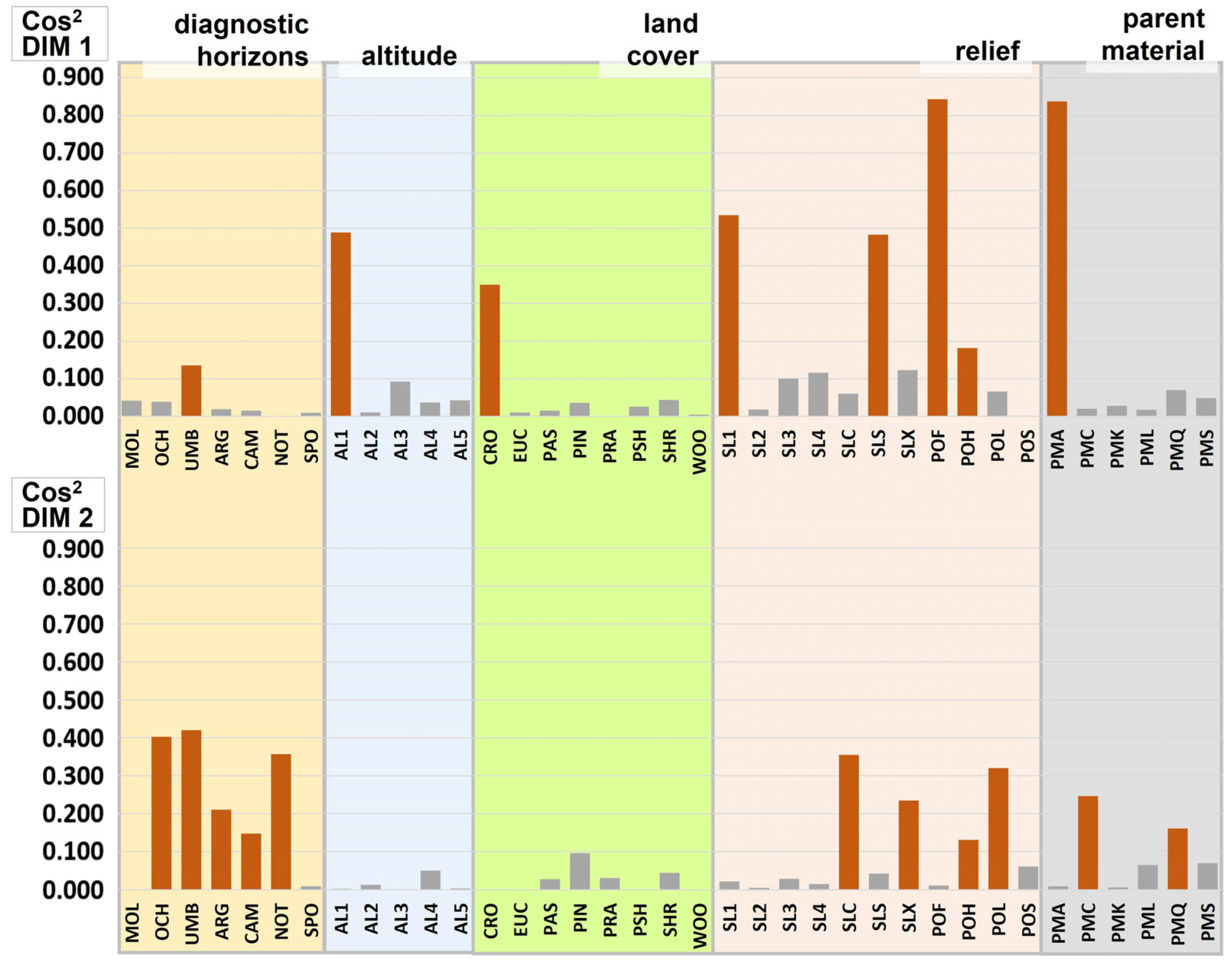
The squared cosine values of each of the categories, for dimensions 1 or 2, are shown in Figure 3.
The variables associated with climatic factors (altitude) and biotic factors (land cover) were those that, to a lesser extent, included categories that contributed significantly to one of the two main dimensions of the MCA. This preliminary analysis highlighted the importance of the relief factor. Among the land cover categories, “cropland” is the only one that contributes, above the average value of cos2, to either of the two main dimensions, specifically, Dim 1. Soil categories such as umbric (UMB) and ochric (OCH) epipedons, argillic (ARG), and cambic (CAM) endopedons, as well as the absence of any diagnostic subsurface horizon (NOT), contribute above the average value of cos2 to Dim 2.
These five soil categories were then subjected to a bivariate analysis with the land cover categories. The results of this bivariate Chi-square test (p < 0.05) are summarized in contingency Table 3 and Table 4.
The land covers associated with agricultural and livestock uses (croplands, pasturelands, and prairies) showed a prevalence of the ochric horizon, contrasting with forest land covers such as Eucalyptus plantations, mixed pasture-shrublands, shrublands, and particularly, pine plantations, for the prevalence of the umbric horizon. Forest uses, both with a strong anthropic influence (Eucalyptus plantations) and natural ones, did not show a significant relationship with any of the superficial diagnostic horizons.
“Prairies” appeared as a category positively related to the presence of soil profiles with an argillic horizon, the opposite case of “pine plantations”. The absence of any subsurface horizon was, however, prevalent in “pine plantations”, unlike “prairies”. “Croplands” and “pasturelands”, on the other hand, showed a prevalence of the Cambic endopedon, which separated them from forest use categories such as “pine plantations”, “mixed pasturelands-shrublands”, and “shrublands”. Once again, “Eucalyptus plantations” and “woodlands” appeared as the worst-defined land cover categories in terms of their relationship with subsurface horizons.
4. Discussion
The multivariate exploratory data analysis defines three groups or clusters of soil profiles (Figure 2a), to which different categories of “soil” and “soil-forming factors” have been associated according to the proximity criterion on 1 and 2 dimensions (Figure 2b). However, when using this criterion, the relatively low explanation of the variance by both dimensions should be considered. In any case, there were numerous proximity relationships between categories that can be explained from a pedological point of view.
The presence of Umbric epipedons and Spodic endopedons in Cluster 1, as well as the absence of any subsurface diagnostic horizon, are pedologically consistent with factors such as forest uses (wooded or shrubby), high altitudes, lithologies that favor the development of acidic and stony soils [36], and landforms associated with erosion and deposition processes, such as steep slopes or high and convex slopes [37].
Cluster 2 included the Ochric and Cambic horizons; both were very close to the category of “prairies” and, to a lesser extent, to “pasturelands”, similarly to the argillic endopedon. Lithologies such as “limestones”, “mixed colluvial”, and “clays” were included in Cluster 2. Such categories are frequently linked to a high contribution of soil exchange bases [38], as well as moderate to strong reliefs, which favor the development of erosive and depositional processes. In limestone massifs, horizons such as Ochric, Mollic, Cambic, and locally, Argillic, are closely linked to rocky outcrops in steeply sloping areas [21], which are not suitable even for livestock land uses. Soils with Argillic horizons usually have high cation exchange capacity as well as moisture retention; both properties may be associated with high soil natural fertility; this fact would favor both agricultural and livestock uses to a greater extent than categories in Cluster 1. However, clayey parent materials, which are frequently associated with Argillic endopedons in the study area [21], can lead to difficulties for tillage and crop rooting [39,40], favoring livestock uses over strictly agricultural ones. These properties may explain the long distance observed between “croplands” and “Argillic” in the MCA. The presence of a Cambic horizon, however, does not generally pose specific limitations to tillage.
The categories of Cluster 3 are characteristic of surfaces of alluvial origin, of flat or very gentle relief, dedicated mainly to agricultural uses, in which, however, there was no clear proximity with categories of any diagnostic horizons except for the relative affinity with the Mollic epipedon.
Clusters 1, 2, and 3 can be well defined from the point of view of the FAO’s Land Suitability Classification [41]. Considering suitability for agricultural and livestock uses, Cluster 3 represented the lands with the highest land suitability classes in the regional context. Cluster 1, on the other hand, included the lands with the lowest classes of suitability: null for agricultural uses, low or moderate for livestock uses, and feasible for forestry ones. Cluster 2 represented an intermediate situation, with generally low agricultural suitability and higher for livestock uses. In this sense, dimension 1 of the MCA discriminated those categories associated with agricultural land covers (croplands) from those associated with other uses. Dimension 2 could differentiate the categories mostly associated with livestock uses, with frequently steep slopes and relatively fertile soils (cluster 2), from those other areas also with high slopes but with acid soils and low or very low natural fertility (cluster 1).
The results obtained in the multivariate analysis showed the importance of the categories associated with the relief-forming factor. This is coherent with the physiographic characteristics of the territory of Asturias [21]. The slope variables “value” and “shape” determined the soil cover since they are key factors for agricultural uses and the development of erosive processes [37] This explains the high contribution of these two variables to the observed variance. The geomorphological variables are conditioned by the parent material, so it must be assumed that both variables act jointly to a large extent. The nature of the parent material conditions the natural fertility of the soils, particularly in young soils affected by erosion and deposition, and therefore, it conditions the land cover. It is worth mentioning the relatively low importance of the climate, which can be explained locally by the general abundance of rainfall and the moderated temperatures in the studied region. In the study area, climate may be considered a determining factor of major differences in soil development only at the highest altitudes (AL4 category), which may limit biological activity, but even so, they are strongly conditioned in the study area by large existing reliefs. Climate, relief, and lithology largely condition the soil cover, which explains why it appears after the MCA as the factor with the lowest contribution to the variance.
In order to deepen the role of land cover as a soil-forming factor, the results of the multiple correspondence analysis were complemented with a bivariate dependency analysis carried out between surface and subsurface diagnostic horizons and land cover categories. The results indicated that the Ochric horizon was prevalent in soils under agricultural-livestock uses: “croplands” “prairies”, and “pasturelands” (Table 3). This made them significantly different from forest uses such as “pine plantations”, “shrublands”, and “mixed pastureland-shrublands”. These results were largely consistent with the proximities between categories observed in the MCA (Figure 2b). Ochric horizons are commonly associated with continued agricultural use that can degrade Mollic horizons towards Ochric horizons due to net loss of organic matter and/or thickness (by erosion) [20]. In general, the intense biological activity in humid and mild climates favors the rapid turn-over of organic matter and the development of the Ochric epipedon [20]. Such climatic conditions characterize the lowest coastal levels of Asturias [36]. Fanning and Fanning [11] indicated the abundance of Ochric horizons in well-drained forest areas, as is the general case in the territory studied. Additionally, some tasks associated with short-cycle Eucalyptus plantations often involve the complete exposure to erosion of bare soil after felling [42], which may be associated with the predominance of Ochric epipedons by the truncation of Mollic or Umbric epipedons.
The analysis of the Umbric horizon and land covers (Table 3) indicates opposite behavior to that of the ochric horizon. Its frequency was significantly lower than expected in the “crops” category. Bockheim [20] pointed out the presence of herbaceous vegetation, coniferous formations, and acidophilic mountain scrub as favorable factors for the development of the Umbric horizon, which is consistent with what was observed in the study area. Formations of various tree species (pine, Eucalyptus sps.) influence the different acidification levels of the surface horizon [43]. In determining the humification conditions in these soils, the role of frequent forest fires must also be taken into account [36]. The characteristic acidity conditions of the umbric horizon and the scarce soil development favor the association of these soils with uses that are less demanding in terms of natural fertility; these are the cases of “pine plantations” or “shrublands”. In the Spanish Atlantic area, cation leaching is intense in soils under Erica sps. and Calluna vulgaris [44]. Such conditions favor the development of the Umbric epipedon [36]. Heathlands are in fact a significant part of the “shrublands” category in the study area [36]. This is consistent with the observed prevalence of Umbric horizons in “shrublands” and the high affinity of both categories as shown in the MCA. However, when analyzing the differences regarding humification between tree species, the results were not conclusive [45]. This is compatible with the different behavior shown by the tree categories of “pine plantations”, “natural woodlands”, and “Eucalyptus plantations”.
Mollic horizons are remarkably unspecific with respect to land cover categories. Mollic horizons are worldwide associated with grasslands in continental temperate areas, characterized by cold winters and humid-warm summers [46], with most of the plant growth occurring in moist spring [47]. The region under study is outside the main manifestations of this epipedon in the world [36]. The natural vegetation is commonly constituted by deeply rooted perennial grasses and shrubs, which favor a high level of biological activity (bioturbation) in the warmer periods of the year [20], as well as the accumulation of humified organic matter to a considerable depth [48].
In the study region, the presence of soil profiles with Mollic epipedon can be mostly explained by the association of shrublands and pasturelands with shallow but relatively fertile soils, developed on calcareous parent materials at different altitudes [21]. These soils support extensive grazing despite the high rockiness and shallowness; hence, the irregular shrubland-grass cover may differentiate this formation from “pasturelands” and “shrublands”, which developed in more homogeneous soil units. This relative fertility encourages livestock uses and restricts less productive forest uses (as “pine plantations”).
On the other hand, significant relationships were described between various land cover categories and Argillic and Cambic subsurface horizons, as well as their absence (Table 4). The results highlighted the prevalence of the Argillic horizon in the “prairies” category. The low affinity of the Argillic endopedon with the “croplands” category is consistent with the recent age of the alluvial sediments in which croplands mostly occur, since this endopedon requires long periods for its development [49,50,51]. This low affinity is extended to the relief categories of null or very gentle slopes (SL1), which characterize alluvial sediments. The “Prairies” category is frequently associated with gentle to moderate slopes, free drainage, and geomorphologically stable surfaces, where the development of argillic horizons is often favored. At the same time, in the case of soils with argillic horizons and high base saturation (Alfisols [ST]), the high natural fertility and moisture retention capacity allow for the most demanding livestock uses (prairies).
In the case of the Cambic horizon, its distribution in the “pasturelands” and “croplands” categories (more than 40% of these profiles have Cambic) is significantly greater than that in forest categories such as “shrublands”, “mixed pasturelands-shrublands”, and “pine plantations”. The Cambic horizon is the most frequent of the endopedons in the study area, which could suggest its low specificity with respect to the different vegetation categories. Nevertheless, this subsurface horizon is prevalent over the “pastureland” and “cropland” categories, where its frequency is significantly greater than in forest categories such as “shrublands”, “mixed pasturelands-shrublands”, and “pine plantations”.
Two land-use categories showed significantly distinct behaviors regarding the absence of any type of subsurface horizon (Table 4): on the one hand, “pine plantations”, in which the absence of such horizons is prevalent; on the other, “prairies”. in which it is significantly less frequent than expected. The absence of endopedons is, on the other hand, prevalent in “mixed pasturelands-shrublands” which differentiates this category from others, also for livestock use, such as “prairies” and “pasturelands”. This is consistent with generally higher agricultural suitability (moderate available rooting depth) of soils with cambic endopedon; in any case, to the best of our knowledge, the literature does not offer specific relationships with land covers and Argillic and Cambic horizons; indirectly, however, agricultural and forest erosion associated with tillage can favor the mixing of surface-subsurface horizons [52] and even cause a complete solum truncation, particularly on steep slopes. In the case of croplands, the relatively frequent absence of endopedons can be explained by the strong association of these soils with recent alluvial deposits, in which no development other than that of a generally Ochric epipedon has yet been possible.
Together with the Mollic epipedon, the Spodic epipedon lacked a significant contribution to any of the main dimensions of the MCA, so it has been discarded from the bivariate analysis. In any case, the proximity of this endopedon to the characteristic categories of Group 1 can be cited, in particular, to the categories of parent materials “quartzitic” and “sandy”, land covers of “scrubland”, and landforms of “positions of high slope” (Table 4). The proximity between all of them is consistent with the conditions for the formation of Spodic endopedons in the temperate zone [36]. In particular, the “shrublands” category is mostly acidophilic and frequently made up of heaths. In fact, podzol-type soils were early defined as “moderately well-drained soils from cool regions developed under forest and/or heathland” [53], and they are favored by acidifying litter (heather and other Ericaceae; conifers; or Eucalyptus sps.) [54] and mor-type humus [55]. Similarly, human influence can accelerate the podsolization process by cultivating acidifying species [38].
Two categories of forest land cover, “Eucalyptus plantations” and “natural woodlands”, are the ones that, to a lesser extent, show dependency relationships with subsurface horizons. In general, the presence of natural woodlands in the study area is restricted to soils that are excluded from agricultural use due to climate (high altitude) or steep slopes, or due to their shallowness, high rockiness and/or stoniness, or their extreme acidity. On the other hand, Eucalyptus plantations are limited to coastal areas (with milder winters), where, due to similar edaphic limitations (shallowness, high rockiness or stoniness, acidity), these soils are usually excluded from agricultural use [21]. It should be noted that these soil properties are not directly expressed in the definition of subsurface diagnostic horizons according to the Soil Taxonomy [19].
It can be considered that a precise definition of soil-land cover relationships is strongly conditioned by the key influence of climate, relief, and lithology factors on the land cover itself. The “soil-land cover” relationship can be reciprocal, in the sense that both can behave as a “cause” and as an “effect” with respect to the other. The unique influence of plant cover on the soil is mainly based on the contribution and biochemical evolution of fresh organic matter. This influences soil morphological and physicochemical properties that discriminate, among other horizons, Ochric, Umbric, or Mollic epipedons. On the other hand, the influence of the “soil” in the “land cover” is based on the fact that the presence of certain horizons (always together with other environmental factors) determines the choice of these soils for different types of agricultural or forestry uses. This refers especially to subsurface horizons such as the Argillic or the Cambic. Their presence in soils generally favors more demanding uses from an edaphic point of view, such as croplands or prairies, since they tend to have higher natural fertility due to their relatively high cation exchange and moisture retention capacities, among other parameters.
5. Conclusions
This work developed an approach for the application of Jenny’s equation to a real scenario based on a statistical analysis of categorical variables. It was specifically oriented to reveal and pedologically interpret objective relationships between diagnostic horizons, as the “soil” product of the equation, and land covers, as the “organisms” factor. The relationship between product and factor was attempted to be resolved by assuming the function “f” of the equation in terms of statistical dependence.
The influence that climate, relief, and lithology exert on land cover, without this variable reciprocally influencing them, can explain the limited role that land cover plays in the multivariate analysis. The results of this analysis indicated, however, similar behaviors between certain land cover categories and diagnostic horizons, which suggested the dual role of land cover: as a “cause” of soil properties and as an “effect” of such properties. This role was evaluated by means of bivariate analysis.
Land cover categories associated with farming use, such as “croplands”, “pasturelands”, and “prairies”, showed dependence relationships with Ochric epipedons. On the other hand, categories associated with forest uses such as “pine plantations”, “mixed pastures-shrublands”, and “shrublands” presented relationships with Umbric epipedons. The pedological interpretation of such relationships allowed for considering the land cover as a “cause” or determining factor of the presence of one or another type of surface diagnostic horizon. Other observed relationships can be interpreted based on the fact that certain soil diagnostic horizons condition the land cover; in these cases, therefore, land cover is assumed to be an “effect” of the “soil” variable. Thus, the presence of diagnostic subsurface horizons such as Argillic or Cambic can be associated with the prevalence of farming land uses. Specifically, this research verified the prevalence of Argillic horizons in the “prairies” category, of Cambic horizons in “croplands” and “pasturelands”, and the prevalence of soils without endopedon in forest land covers such as “pine plantations”, “mixed pastures-shrublands”, and “shrublands”. The obtained relationships are mostly consistent with the pedological literature and, to our knowledge, have not been previously described by means of statistical tools.
This research demonstrates the potential utility of land cover, one of the environmental elements whose spatial representation is more reliable and generalized, as an indicator of the prevalence of different diagnostic horizons in a specific region. An accurate definition of variables and categories, based on the information provided by the widely available descriptions of soil profiles, allows for the adaptation of the methodology presented in this work to other regions, thus contributing to the development of models oriented to the challenging task of soil spatial representation.
Author Contributions
Conceptualization, M.R.-R.; methodology, M.R.-R.; investigation, M.R.-R. and A.O.-M.; data curation, M.R.-R., V.C. and A.O.-M.; writing-original draft preparation, M.R-R.; writing-review and editing, M.R.-R., A.O.-M. and V.C. All authors have read and agreed to the published version of the manuscript.
Funding
Víctor Cicuéndez was supported by a post-doctoral Juan de la Cierva fellowship (FJC2021-046735-I) funded by the Spanish Ministerio de Ciencia e Innovación MCIN/AEI/10.13039/501100011033 and by the European Union’s «NextGenerationEU»/PRTR».
Institutional Review Board Statement
Not applicable.
Informed Consent Statement
Not applicable.
Data Availability Statement
Not applicable.
Acknowledgments
The authors wish to thank Ricardo Pérez-Ochoa (Government of Asturias) and José Gumuzzio for facilitating access to basic soil information, Javier Rodríguez Alonso (INIA, Madrid), for managing georeferenced data in Figure 1, and Felipe Yunta-Mezquita (JRC-European Commission) for his recommendations for the preparation of this document.
Conflicts of Interest
The authors declare no conflict of interest.
References
- Florinsky, I.V. The Dokuchaev Hypothesis as a Basis for Predictive Digital Soil Mapping (On the 125th Anniversary of Its Publication). Eurasian Soil Sci. 2012, 45, 445–451. [Google Scholar] [CrossRef]
- Jenny, H. Factors of Soil Formation; McGraw-Hill: New York, NY, USA, 1941; p. 281. [Google Scholar] [CrossRef]
- Wilding, L.P.; Smeck, N.E.; Hall, G.F. Developments in Soil Science. In Pedogenesis and Soil Taxonomy. I. Concepts and Interactions; Wilding, L.P., Smeck, N.E., Hall, G.F., Eds.; Elsevier Science Publishers B.V.: Amsterdam, The Netherlands, 1983; pp. 117–140. ISBN 978-0-444-42100-5. [Google Scholar]
- Stockmann, U.; Minasny, B.; MacBratney, A.B. Quantifying Processes of Pedogenesis. Adv. Agron. 2011, 113, 293–323. [Google Scholar] [CrossRef]
- Bockheim, J.G.; Gennadiyev, A.N.; Hammer, R.D.; Tandarich, J.P. Historical development of key concepts in pedology. Geoderma 2005, 124, 23–36. [Google Scholar] [CrossRef]
- Phillips, J.D. Stability implications of the state factor model of soils as a nonlinear dynamical system. Geoderma 1993, 58, 1–15. [Google Scholar] [CrossRef]
- Giupponi, L.; Leoni, V.; Pedrali, D.; Zuccolo, M.; Cislaghi, A. Plant cover is related to vegetation and soil features in limestone screes colonization: A case study in the Italian Alps. Plant Soil. 2022, 483, 495–513. [Google Scholar] [CrossRef]
- Porder, S. How Plants Enhance Weathering and How Weathering is Important to Plants. Elements 2019, 15, 241–246. [Google Scholar] [CrossRef]
- Grunwald, S. Future of Soil Science. In The Future of Soil Science; Hartemink, A., Ed.; IUSS International Union of Soil Sciences: Wageningen, The Netherlands, 2006; pp. 51–53. ISBN 90-71556-16-6. [Google Scholar]
- Fitzpatrick, E.A. Soils, Their Formation, Classification and Distribution; Longman Inc.: New York, NY, USA, 1983; ISBN 978-0-582-30116-0. [Google Scholar]
- Fanning, D.S.; Fanning, M.C.B. Soil: Morphology, Genesis and Classification; John Wiley & Sons: New York, NY, USA, 1989; p. 416. ISBN 978-0-471-89248-9. [Google Scholar]
- Jenny, H. The Soil Resource, Origin and Behaviour; Springer: New York, NY, USA, 1980; p. 368. [Google Scholar] [CrossRef]
- Ugolini, F.C.; Edmonds, R.L. Soil Biology. In Pedogenesis and Soil Taxonomy. I. Concepts and Interactions; Wilding, L.P., Smeck, N.E., Hall, G.F., Eds.; Elsevier Science Publishers B.V.: Amsterdam., The Netherlands, 1983; Chapter 7; pp. 193–231. ISBN 978-0-444-42100-5. [Google Scholar]
- Jenny, H. Role of the Plant Factor in the Pedogenic Functions. Ecology 1958, 39, 5–16. [Google Scholar] [CrossRef]
- Hironaka, M.; Fosberg, M.A.; Neiman, K.E., Jr. The relationship between soils and vegetation. In Proceedings of the Symposium on Management and Productivity of Western-Montane Forest Soils, Boise, ID, USA, 10–12 April 1990; pp. 29–31. [Google Scholar]
- Roy, P.S.; Dwivedi, R.S.; Vijayan, D. Remote Sensing Applications. Government of India, National Remote Sensing Centre. Indian Space Research Organisation. Available online: https://www.nrsc.gov.in/sites/default/files/pdf/ebooks/Chap_2_LULC.pdf (accessed on 24 January 2023).
- Rossiter, D.G. Soil mapping today: Computer-generated predictive soil maps–their role in soil survey and land evaluation. Agric. Dev. 2021, 44. Available online: https://www.isric.org/sites/default/files/Ag4Dev44-Article5.pdf (accessed on 24 January 2023).
- IUSS Working Group-WRB. World Reference Base for Soil Resources. International Soil Classification System for Naming Soils and Creating Legends for Soil Maps; World Soil Resources Reports No. 106; FAO: Rome, Italy, 2014; p. 181. ISBN 978-92-5-108369-7. [Google Scholar]
- Soil Survey Staff. Keys to Soil Taxonomy, 12th ed.; USDA—Natural Resources Conservation Service: Washington, DC, USA, 2014; p. 362. [Google Scholar]
- Bockheim, J.G. Soil Geography of the USA: A Diagnostic-Horizon Approach; Springer International Publishing: Cham, Switzerland, 2014; p. 320. ISBN 978-3-319-06668-4. [Google Scholar]
- Rodríguez-Rastrero, M. Los suelos de Asturias (España): Un enfoque basado en las relaciones entre factores formadores y horizontes de diagnóstico. Ph.D. Thesis, Autonomous University of Madrid, Madrid, Spain, January 2016. (In Spanish). Available online: https://repositorio.uam.es/handle/10486/671738 (accessed on 3 August 2022).
- Chazarra, A.; Flórez-García, E.; Peraza, B.; Tohá-Rebull, T.; Lorenzo-Mariño, B.; Criado, E.; Moreno-García, J.V.; Romero-Fresneda, R.; Botey, M.R. Mapas climáticos de España (1981–2010) y ETo (1996–2016). 2018. Available online: http://www.aemet.es/es/conocermas/recursos_en_linea/publicaciones_y_estudios/publicaciones/detalles/MapasclimaticosdeEspana19812010 (accessed on 18 September 2022).
- Field Book for Describing and Sampling Soils, Version 2.0; Schoeneberger, P.J.; Wysocki, D.A.; Benham, E.C.; Broderson, W.D. (Eds.) Natural Resources Conservation Service, National Soil Survey Center: Lincoln, NE, USA, 2002. [Google Scholar]
- Buol, S.W.; Southard, R.J.; Graham, R.J.; McDaniel, P.A. Soil Genesis and Classification, 6th ed.; Wiley-Blackwell: Oxford, UK, 2011; p. 527. [Google Scholar] [CrossRef]
- Nater, E.A.; Jelinski, N.A. Temperate Region Soils. In Reference Module in Earth Systems and Environmental Sciences; Elsevier: Amsterdam, The Netherlands, 2014; Reference Collection. [Google Scholar] [CrossRef]
- Huggett, R.J. Soil chronosequences, soil development, and soil evolution: A critical review. Catena 1998, 32, 155–172. [Google Scholar] [CrossRef]
- European Union. Copernicus Land Monitoring Service. European Environment Agency (EEA). Available online: https://land.copernicus.eu/pan-european/corine-land-cover/clc2018 (accessed on 20 September 2022).
- Ferrer, C.; San Miguel, A.; Olea, L. Nomenclátor básico de pastos en España. Pastos 2001, 2, 7–44. Available online: http://polired.upm.es/index.php/pastos/article/view/1694 (accessed on 21 December 2017).
- Martínez-Fernández, A.; Argamentería, A.; De la Roza, B. Manejo de Forrajes Para Ensilar; Servicio Regional de Investigación y Desarrollo Agroalimentaria (SERIDA) del Principado de Asturias: Villaviciosa, Spain, 2014; p. 280. ISBN 978-84-617-3224-0. [Google Scholar]
- Blanco, E.; Casado, M.A.; Costa, M.; Escribano, R.; García, M.; Génova, M.; Gómez, A.; Gómez, F.; Moreno, J.C.; Morla, C.; et al. Los Bosques Ibéricos; Una Interpretación Geobotánica, Ed.; Planeta: Barcelona, Spain, 2005; p. 597. ISBN 978-8-408-05820-5. [Google Scholar]
- Ortega, M.E.; De la Mano, D.; Fernández, S.; Garrido, B. El Monte en Asturias. Consejería de Medio Rural y Pesca. Dirección General de Política Forestal. Gobierno del Principado de Asturias, Spain. 2011. Available online: https://www.asturias.es/Asturias/descargas/PDF_TEMAS/Agricultura/Politica%20Forestal/el_monte_en_asturias.pdf (accessed on 21 December 2017).
- González-Taboada, F.; Anadón-Álvarez, R. Análisis de Escenarios de Cambio Climático en Asturias (Roqueñi y Orviz, Coord.); Gobierno del Principado de Asturias: Oviedo, Spain, 2011; ISBN 978-84-694-2848-1. [Google Scholar]
- Abdi, H.; Valentin, D. Multiple Correspondence Analysis. In Encyclopedia of Measurement and Statistics; Salkind, N., Ed.; University of Texas: Dallas, TX, USA, 2007; Available online: https://personal.utdallas.edu/~herve/Abdi-MCA2007-pretty.pdf (accessed on 20 February 2023).
- Lê, S.; Josse, J.; Husson, F. FactoMineR: An R Package for Multivariate Analysis. J. Stat. Softw. 2008, 25, 1–18. [Google Scholar] [CrossRef] [Green Version]
- STHDA. Statistical Tools for High-Throughput Data Analysis. Available online: http://www.sthda.com/english/articles/31-principal-component-methods-in-r-practical-guide/114-mca-multiple-correspondence-analysis-in-r-essentials/ (accessed on 2 February 2023).
- Carballas, T.; Rodríguez-Rastrero, M.; Artieda, O.; Gumuzzio, J.; Díaz-Raviña, M.; Martin, Á. Soils of the temperate humid zone. In The Soils of Spain; Gallardo, J.F., Ed.; Springer International Publishing: Cham, Switzerland, 2016. [Google Scholar] [CrossRef]
- Sun, L.; Guo, H.; Liu, B.; Wu, S.; Weckler, P.R.; Yang, J. Characterizing erosion processes on a convex slope based on 3D reconstruction method. Geoderma 2021, 402, 115364. [Google Scholar] [CrossRef]
- Duchaufour, P.; Souchier, B. Edafología. I: Edafogénesis y Clasificación (Spanish versión by Carballas, T. y Carballas, M.); Editorial Masson: Barcelona, Spain, 1984; p. 483. ISBN 84-311-0344-2. [Google Scholar]
- Zhou, Y.; Boutton, T.W.; Wu, X.B. Subsurface soil horizons drive landscape patterns of woody patches in a subtropical savanna. In Proceedings of the Society for Range Management (SRM), Conference Proceedings, 2016, Corpus Christi, TX, USA, 31 January–4 February 2016. [Google Scholar]
- Kosmas, C.; Danalatos, N.; Cammeraat, L.; Chabart, M.; Diamantopoulos, J.; Farand, R.; Gutiérrez, L.; Jacob, A.; Marques, H.; Martínez-Fernández, J.; et al. The effect of land use on runoff and soil erosion rates under Mediterranean conditions. Catena 1997, 29, 45–59. [Google Scholar] [CrossRef]
- Verheye, W.; Koohafkan, P.; Nachtergaele, F. The FAO Guidelines for Land Evaluation-Land Use, Land Cover and Soil Sciences-Vol. II. 2003. UNESCO-EOLSS. Available online: http://eolss.net/Sample-Chapters/C19/E1-05-02-03.pdf (accessed on 21 February 2023).
- Fernández, C.; Vega, J.A.; Gras, J.M.; Fonturbel, T.; Cuiñas, P.; Dambrine, E.; Alonso, M. Soil erosion after Eucalyptus globulus clearcutting: Differences between logging slash disposal treatments. For. Ecol. Manag. 2004, 195, 85–95. [Google Scholar] [CrossRef]
- Álvarez, E.; Martínez, A.; Veiga, A. Composición iónica de la disolución de suelos de Galicia: Relación con el tipo de cubierta arbórea y material de partida. Ecología 1992, 6, 17–27. [Google Scholar]
- Calvo de Anta, R.M.; Díaz-Fierros, F. Consideraciones acerca de la acidificación de los suelos de la zona húmeda española a través de la vegetación. An. Edaf. Agrob. 1981, 40, 411–425. [Google Scholar]
- Calvo de Anta, R.M.; Paz, A.; Díaz-Fierros, F. Nuevos datos sobre la influencia de la vegetación en la formación del suelo en Galicia (I). An. Edaf. Agrobiol. 1979, 38, 1675–1691. [Google Scholar]
- Eswaran, H.; Reich, P.F. World soil map. In Encyclopedia of Soils in the Environment; Four-Volume set; Hillel, D., Ed.; Elsevier: New York, NY, USA, 2005; pp. 352–365. ISBN 978-0-123-48530-4. [Google Scholar]
- Kögel-Knaber, I.; Amelung, W. Dynamics, Chemistry, and Preservation of Organic Matter in Soils. pp. 157–215; In Treatise on Geochemistry, 2nd ed.; Holland, H.D., Turekian, K.K., Eds.; Elsevier: Oxford, UK, 2014; p. 12. ISBN 978-0-080-95975-7. [Google Scholar]
- Hillel, D. Soil in the Environment; Elsevier Academic Press: Burlington, MA, USA, 2008; p. 307. [Google Scholar] [CrossRef]
- Sauer, D.; Schülli-Maurer, I.; Sperstad, R.; Sørensen, R.; Stahr, K. Albeluvisol development with time in loamy marine sediments of southern Norway. Quat. Int. 2009, 209, 31–43. [Google Scholar] [CrossRef]
- Vidic, N.J. Soil-age relationships and correlations: Comparison of chronosequences in the Ljubljana Basin, Slovenia and USA. Catena 1998, 34, 113–129. [Google Scholar] [CrossRef]
- Papiernik, S.K.; Lindstrom, M.J.; Schumacher, T.E.; Schumacher, J.A.; Malo, D.D.; Lobb, D.A. Characterization of soil profiles in a landscape affected by long term tillage. Soil Tillage Res. 2007, 93, 335–345. [Google Scholar] [CrossRef]
- Sanborn, P.; Lamontagne, L.; Hendershot, W. Podzolic soils of Canada: Genesis, distribution, and classification. Can. J. Soil Sci. 2011, 91, 843–880. [Google Scholar] [CrossRef]
- Buurman, P.; Jongmans, A.G. Podzolization–An additional paradigm. Edafología 2002, 9, 107–114. [Google Scholar]
- Schaetzl, R.J.; Isard, S.A. Regional-scale relationships between climate and strength of podzolization in the Great Lakes Region, North America. Catena 1996, 28, 47–69. [Google Scholar] [CrossRef]
- Lundström, U.S.; Van Breemen, N.; Bain, D. The podsolization process. A review. Geoderma 2000, 94, 91–107. [Google Scholar] [CrossRef]
Figure 1.
Location of the Region (Principality) of Asturias (Northern Spain), with the soil and land cover sampling points. Both base images obtained from Instituto Geográfico Nacional (IGN); https://www.ign.es/iberpix/visor/ (Accessed on 3 August 2022).
Figure 1.
Location of the Region (Principality) of Asturias (Northern Spain), with the soil and land cover sampling points. Both base images obtained from Instituto Geográfico Nacional (IGN); https://www.ign.es/iberpix/visor/ (Accessed on 3 August 2022).
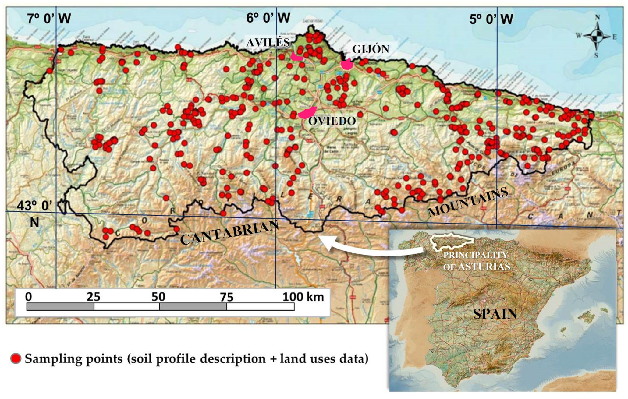
Figure 2.
Cluster factor map for soil profiles (a), and categories of “soil” and “soil forming factors” in the plane of dimensions 1 and 2 (b). Illustrative variables are soil diagnostic horizons and land cover.
Figure 2.
Cluster factor map for soil profiles (a), and categories of “soil” and “soil forming factors” in the plane of dimensions 1 and 2 (b). Illustrative variables are soil diagnostic horizons and land cover.
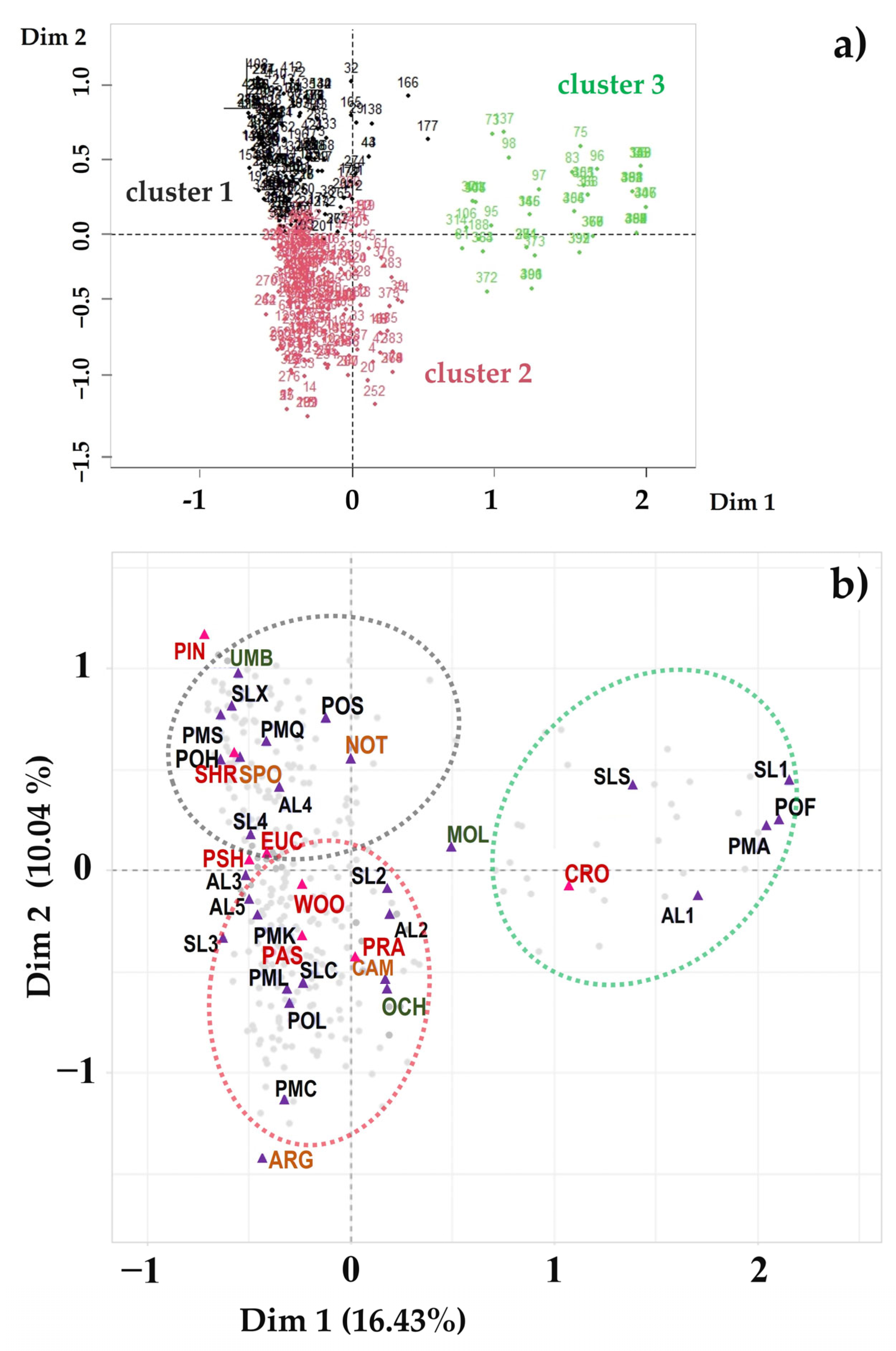
Figure 3.
Cos2 values for all categories of the variables used in the MCA. In reddish-brown, those values above the average of each axis. Categories are organized according to soil and forming factors.
Figure 3.
Cos2 values for all categories of the variables used in the MCA. In reddish-brown, those values above the average of each axis. Categories are organized according to soil and forming factors.

Table 1.
Criteria for definition of land cover categories based on CORINE Land Cover classes.
| CORINE Land Cover (CLC) Classes | CORINE Code | Class Definitions | |
|---|---|---|---|
| According to CLC (*) | Specifications for the Territory of Asturias | ||
| Non-irrigated arable land | 211 | Cultivated land under rainfed agricultural uses, for non-permanent crops of annual harvest, normally under crop rotation. It includes cereals, tubers, legumes, oilseeds, as well as forages (alfalfa, grass for silage or hay production). | Regularly tilled soils, commonly used as monophyte forage crops by mowing [28], with horticultural crops and orchards (frequently kiwifruit orchards). |
| Pastures, meadows and other permanent grasslands under agricultural use | 231 | Permanent grasslands characterized by agricultural use or heavy human disturbance, dominated by grasses. Normally, for grazing (pastures) or mechanical grass harvesting (meadows). | Sown polyphyte grasslands, evergreen mixtures of grasses and legumes, used by mowing or grazing [28], depending on whether general slopes are greater than 14% or not, which determines mechanization capacity [29]. |
| Broad-leaved forest | 311 | Pure or mixed stands of beech, oak, hornbeam, lime, maple, ash, poplar or birch species, as well as riparian and gallery woodlands; chestnut trees and plantations of Eucalyptus. | Mature and dense forest formations, mostly of beech, oak and mixed Atlantic forests according to Blanco et al. [30]. Plantations of Eucalyptus, mainly constituted by E. globulus [31], are considered apart given its anthropic character, which frequently supposes a profound alteration of natural soils. |
| Coniferous forest | 312 | Include mature coniferous (needle-leaved) forests of natural or anthropogenic origin, as well as young plantations of coniferous trees reaching 5 m height. | Conifer plantations, mainly constituted by Pinus radiata and P. sylvestris [31]. |
| Natural grassland | 321 | Low productivity grasslands under no or moderate human influence. Often situated in steep slopes; frequently including rocky areas or patches of other (semi-)natural vegetation, with sporadically (<30% surface) occurring ligneous vegetation including shrubs. | Semi-natural herbaceous communities of variable density, mainly used for grazing [28]. |
| Moors and heathland | 322 | Dense vegetation covers of shrubs (heathers, brooms, gorse and others) and herbaceous in Atlantic, sub-Atlantic and sub-continental areas. | Shrubby formations less than 2 m, included in Cytisetea scopario-striati, and Calluno-Ulicetea communities [28]. It includes high altitude grasslands and natural herbaceous communities mixed with shrubs, exclusively dedicated to seasonal grazing. |
(*) Updated CLC illustrated nomenclature guidelines. European Environment Agency (version 10 May 2019).
Table 2.
Summary of variables and categories for soil and soil forming factors.
| Clorpt Components | Variables | Categories | MCA Code | n |
|---|---|---|---|---|
| SOIL (S) | Surface horizons (nominal) | Mollic | MOL | 62 |
| Ochric | OCH | 230 | ||
| Umbric | UMB | 132 | ||
| Subsurface horizons (nominal) | Argillic | ARG | 40 | |
| Cambic | CAM | 140 | ||
| no subsurface horizon | NOT | 231 | ||
| Spodic | SPO | 13 | ||
| CLIMATE (Cl) | Altitude (interval) | >50 | AL1 | 61 |
| 50–200 | AL2 | 92 | ||
| 200–600 | AL3 | 110 | ||
| 600–1000 | AL4 | 99 | ||
| >1000 | AL5 | 62 | ||
| ORGANISMS (o) | Land cover (nominal) | crops | CRO | 99 |
| Eucalyptus plantations | EUC | 24 | ||
| pasturelands | PAS | 87 | ||
| pine plantations | PIN | 28 | ||
| prairies | PRA | 58 | ||
| mixed pasture/shrublands | PSH | 43 | ||
| shrublands | SHR | 51 | ||
| natural woodlands | WOO | 34 | ||
| RELIEF (r) | Slope value (interval) | <2% | SL1 | 44 |
| 3–16% | SL2 | 154 | ||
| 17–50% | SL3 | 180 | ||
| >50% | SL4 | 46 | ||
| Slope shape (nominal) | concave slope | SLC | 225 | |
| convex slope | SLX | 85 | ||
| straight slope | SLS | 114 | ||
| Relative position (nominal) | floodplains | POF | 68 | |
| high slopes | POH | 132 | ||
| low slopes | POL | 182 | ||
| summits | POS | 42 | ||
| PARENT MATERIAL (p) | Lithology (nominal) | mixed alluvium | PMA | 70 |
| clayey materials | PMC | 68 | ||
| mixed colluvium | PMK | 51 | ||
| limestones | PML | 65 | ||
| quartzitic sandy materials | PMQ | 124 | ||
| slates | PMS | 46 |
n = number of soil profiles within categories.
Table 3.
Contingency tables: coincidences of soil profiles with Ochric and Umbric surface diagnostic horizons with land cover categories.
Table 3.
Contingency tables: coincidences of soil profiles with Ochric and Umbric surface diagnostic horizons with land cover categories.
| Surf_HOR Categories | Land Cover Categories (CORINE Equivalences) | ||||||||
|---|---|---|---|---|---|---|---|---|---|
| CRO (211) | EUC (311) | PAS (321) | PIN (312) | PRA (231) | PSH (322) | SHR (322) | WOO (311) | ||
| OCH n = 230 | Count | 66 a | 10 bc | 57 a | 5 d | 39 a | 15 c | 17 cd | 21 ab |
| Expected count | 52 | 14 | 46 | 18 | 32 | 20 | 29 | 18 | |
| % Within Surf_HOR | 30 | 4 | 24 | 2 | 17 | 7 | 7 | 9 | |
| % Within Land_cover | 83 | 45 | 75 | 18 | 78 | 47 | 37 | 72 | |
| % Total | 19 | 3 | 15 | 1 | 11 | 4 | 5 | 6 | |
| UMB n = 132 | Count | 14 a | 12 bc | 19 a | 23 d | 11 a | 17 c | 28 cd | 8 ab |
| Expected count | 30 | 8 | 27 | 10 | 18 | 12 | 17 | 11 | |
| % Within Surf_HOR | 11 | 9 | 14 | 17 | 8 | 13 | 22 | 6 | |
| % Within Land_cover | 17 | 55 | 25 | 82 | 22 | 53 | 63 | 28 | |
| % Total | 4 | 3 | 5 | 6 | 3 | 5 | 8 | 2 | |
OCH: Ochric; UMB: Umbric; CRO: croplands; EUC: Eucalyptus plantations; PAS: pasturelands; PIN: pine plantations; PRA: prairies; PSH: mixed pasturelands-shrublands; SHR: shrublands; WOO: natural woodlands. Subscript letters a–d, denote subsets of land cover categories whose column proportions do not differ significantly from each other at the 0.05 level.
Table 4.
Contingency tables: coincidences of soil profiles with Argillic, Cambic, and soil profiles lacking any subsurface diagnostic horizons, with land cover categories.
Table 4.
Contingency tables: coincidences of soil profiles with Argillic, Cambic, and soil profiles lacking any subsurface diagnostic horizons, with land cover categories.
| SubSurf_HOR Categories | Land Cover Categories (CORINE Equivalences) | ||||||||
|---|---|---|---|---|---|---|---|---|---|
| CRO (211) | EUC (311) | PAS (321) | PIN (312) | PRA (231) | PSH (322) | SHR (322) | WOO (311) | ||
| ARG n = 40 | Count | 6 ab | 3 bc | 7 ab | 0 a | 14 c | 4 abc | 4 ab | 2 ab |
| Expected count | 10 | 2 | 8 | 3 | 6 | 4 | 4 | 3 | |
| % Within SubSurf_HOR | 15 | 8 | 18 | 0 | 35 | 10 | 10 | 5 | |
| % Within Land_cover | 6 | 14 | 8 | 0 | 24 | 9 | 9 | 6 | |
| % Total | 2 | 1 | 2 | 0 | 3 | 1 | 1 | 1 | |
| CAM n = 139 | Count | 43 a | 8 abc | 37 a | 3 d | 21 ac | 9 bcd | 8 bd | 10 abcd |
| Expected count | 33 | 8 | 29 | 9 | 20 | 15 | 15 | 11 | |
| % Within SubSurf_HOR | 31 | 6 | 27 | 2 | 15 | 7 | 6 | 7 | |
| % Within Land_cover | 44 | 36 | 43 | 11 | 36 | 21 | 18 | 31 | |
| % Total | 11 | 2 | 9 | 1 | 5 | 2 | 2 | 2 | |
| NOT n = 231 | Count | 49 ab | 11 abc | 42 ab | 24 d | 23 b | 30 cd | 32 cd | 20 ac |
| Expected count | 55 | 12 | 49 | 15 | 33 | 24 | 25 | 18 | |
| % Within SubSurf_HOR | 21 | 5 | 18 | 10 | 10 | 13 | 14 | 9 | |
| % Within Land_cover | 50 | 50 | 49 | 89 | 40 | 70 | 73 | 63 | |
| % Total | 12 | 3 | 10 | 6 | 6 | 7 | 8 | 5 | |
ARG: Argillic; CAM: Cambic; NOT: absence of any endopedon; CRO: croplands; EUC: Eucalyptus plantations; PAS: pasturelands; PIN: pine plantations; PRA: prairies; PSH: mixed pasturelands-shrublands; SHR: shrublands; WOO: natural woodlands. Subscript letters a–d, denote subsets of land cover categories whose column proportions do not differ significantly from each other at the 0.05 level.
Disclaimer/Publisher’s Note: The statements, opinions and data contained in all publications are solely those of the individual author(s) and contributor(s) and not of MDPI and/or the editor(s). MDPI and/or the editor(s) disclaim responsibility for any injury to people or property resulting from any ideas, methods, instructions or products referred to in the content. |
© 2023 by the authors. Licensee MDPI, Basel, Switzerland. This article is an open access article distributed under the terms and conditions of the Creative Commons Attribution (CC BY) license (https://creativecommons.org/licenses/by/4.0/).
Share and Cite
MDPI and ACS Style
Rodríguez-Rastrero, M.; Ortega-Martos, A.; Cicuéndez, V. Soil and Land Cover Interrelationships: An Analysis Based on the Jenny’s Equation. Soil Syst. 2023, 7, 31. https://doi.org/10.3390/soilsystems7020031
AMA Style
Rodríguez-Rastrero M, Ortega-Martos A, Cicuéndez V. Soil and Land Cover Interrelationships: An Analysis Based on the Jenny’s Equation. Soil Systems. 2023; 7(2):31. https://doi.org/10.3390/soilsystems7020031
Chicago/Turabian StyleRodríguez-Rastrero, Manuel, Almudena Ortega-Martos, and Víctor Cicuéndez. 2023. "Soil and Land Cover Interrelationships: An Analysis Based on the Jenny’s Equation" Soil Systems 7, no. 2: 31. https://doi.org/10.3390/soilsystems7020031