Terrain Effects on the Spatial Variability of Soil Physical and Chemical Properties

Abstract

Understanding topography effects on soil properties is vital to modelling landscape hydrology and establishing sustainable on-field management practices. This research focuses on an arable area (117 km²) in Southwestern Ethiopia where agricultural fields and bush cover are the dominant land uses. We postulate that adapting either of the soil data resources, coarse resolution FAO-UNESCO (Food and Agriculture Organization of the United Nations Educational, Scientific and Cultural Organization) soil data or pedo-transfer functions (PTFs) is not reliable to indicate future watershed management directions. The FAO-UNESCO data does not account for scale issues and assigns the same soil property at different landscape gradients. The PTFs, on the other hand, do not account for environmental effects and fail to provide all the required data. In this regard, mapping soil property spatial dynamics can help understand landscape physicochemical processes and corresponding land use changes. For this purpose, soil samples were collected across the watershed following a gridded sampling scheme. In areas with heterogeneous topography, soil is spatially variable as influenced by land use and slope. To understand the spatial variation, this research develops indicators, such as topographic index, soil topographic wetness index, elevation, aspect, and slope. Pearson correlation (r), among others, was used to investigate terrain effects on selected soil properties: organic matter (OM), available water content (AWC), sand content (%), clay content (%), silt content (%), electrical conductivity (EC), moist bulk density (MBD), and saturated hydraulic conductivity (Ksat). The results show that there were statistically significant correlations between elevation-based variables and soil physical properties. Among the variables considered, the ‘r’ value between topographic index and soil attributes (i.e., OM, EC, AWC, sand, clay, silt, and Ksat) were 0.66, 0.5, 0.7, 0.55, 0.62, 0.4, and 0.66, respectively. In conclusion, while understanding topography effects on soil properties is vital, implementing either FAO-UNESCO or PTFs soil data do not provide appropriate information pertaining to scale issues.

1. Introduction

Soils vary widely as a function of their position on the landscape [1,2,3] and agricultural management, land use, and cultivation intensity [4,5]. As a result, identification of landscape features is an important tool used by pedologists in soil classification and mapping [6]. To account for these unpredicted soil property spatial variation and relationships, studies [7] recommend employing geostatistical analysis tools. Ceddia et al. [6] highlighted that soil physical attributes are related to topography over a landscape and it was viable to use cokriging point iteration with topography as an auxiliary variable. For example, based on a grid scheme field observation, Vauclin et al. [8] used geostatistical concepts employing krige and cokrige to assess the spatial variability of silt, sand, clay, and available water content (AWC). In addition, the spatial variation of soil properties can be determined using pedo-transfer functions (PTFs) [9].

Pedo-transfer functions are a non-linear multiple regression of combinations of soil physical properties that reproduce soil hydraulic properties. In this context, the soil water characteristics PTFs in the soil-plant-air-water (SPAW) model were used to predict soil characteristics during soil textural classification. Soil databases directly derived from global soil maps are assumed to have a normal soil density and the PTFs of [9] used a relative compaction density equal to unity. In this context, the soil water characteristics PTFs in the soil-plant-air-water (SPAW) model were used to define soil textural classes using data inputs analyzed during a field and laboratory analysis. These datasets included percentage of sand and clay content, organic matter (OM), gravel, and bulk density. There are various PTFs available in the literature that included PTFs built from a collection of USA soil samples [9,10,11] and European soil samples [12].

PTFs are different depending on their required input parameters and underlying equations. They take either the form of lookup tables based on soil textural classes from the available soil maps or the form of continuous functions with soil properties as input [13,14]. The selection of PTFs involved the assessment of model performance criteria and prediction accuracy. According to Gijsman et al. [15], the SPAW soil water characteristics PTFs are further applied to define soil textural classes. However, soil texture, which affects moisture retention and pattern of land use, is thought to vary with catchment topography [16].

Soil physical attributes are related to topographic heterogeneity [6] and changes in soil properties could affect soil water content, vegetation response [17] and the rate of land use change [7,18]. In addition, as an important indicator of topography, terrain slope has a clear effect on erosion rate [6,19], thereby affecting the soil and pattern of land use. According to Opršal et al. [20], environmental factors are more influential in areas with greater topographic heterogeneity. Among these factors, climate, soil properties, and topography would be expected to affect land use change [21], which, in turn, will have a substantial effect on soil properties such as soil texture, fertility and Carbone content [22,23,24].

In general, the way we manage catchment soil and land use may alter the fluxes of water and sediment as it may either reduce soil moisture content and base flow, accelerated overland flow, or increase soil erosion and degradation. This effect is more pronounced in highly rugged areas where there is a significant land disturbance and topographic influences are dominant. In this regard, various studies have been conducted to assess the relation between soil properties and terrain variables [25,26,27,28,29].

However, there is no significant research in the region that follows a bottom-up approach to drive the soil–topography relationship and upscale the result for hydrological modelling. It should also be pointed out that accurate soil physicochemical property characterization is only accurate at the smaller spatial scale; i.e., plot to watershed level rather than basin scales. Fine scale assessment of watershed soil dynamics and explaining data resolution issues in modelling enables management authorities to develop corrective environmental protection and sustainability plans.

To this end, previous studies on the spatial variability of soil properties are either site-specific, coarse scale, or implemented pedo-transfer functions that neither account for environmental effects nor provide all the required data inputs. Our research, on the other hand, maps soil property spatial dynamics to understand landscape physicochemical processes in the area and used in hydrological modeling for future soil and watershed management applications. The significance of the work therefore stems from the fact that we did not rely on our research to use either coarse resolution FAO-soils that assigns the same soil property at different landscape gradients or site-specific and unreliable PTfs. Instead, we developed soil–landscape relation for a tropical catchment in the Rift Valley basin where data are a scarce resource.

Here, two points need to be balanced. Firstly, the indispensability of knowledge of soil properties for planning territorial development and environmental conservation. Secondly, implementation of methodologies that rapidly and effectively capture information about the spatial variability of soils in a way that reduces the need for intensive and expensive sampling [30]. In this regard, the geostatistical approach, which uses probabilistic methods, has been successfully used in soil science for quantitative description of the spatial variability of soil physical and chemical properties [31]. Since topography parameters are known to control water and sediments distribution over the landscape, features such as altitude, slope, and shape are correlated with soil physical properties [3].

To understand the spatial variability of soil and land use in a rugged, mountainous environment of the Rift Valley region, this research extracted indicators from digital elevation models, such as a topographic index, soil topographic wetness index, elevation, aspect, and slope. These indicators were then used to identify the spatial characteristics of soils and analyze the spatial variability as it is affected by climate, soil property, and topography. The use of the digital elevation model increased the predictive accuracy of soil parameters from terrain attributes.

In this paper, we measured the spatial variability of soils across the watershed and evaluated the use of topographic indices to develop explanatory variables. Specific objectives were (1) developing a fine scale soil map of the watershed, (2) spatially correlate soil properties and topographic attributes, and (3) assess the interactive effect of soil, land use type, and slope position on soil physiochemical properties. To improve soil property mapping, we used auxiliary variables that help understand the processes occurring over the landscape and improve the precision of soil mapping.

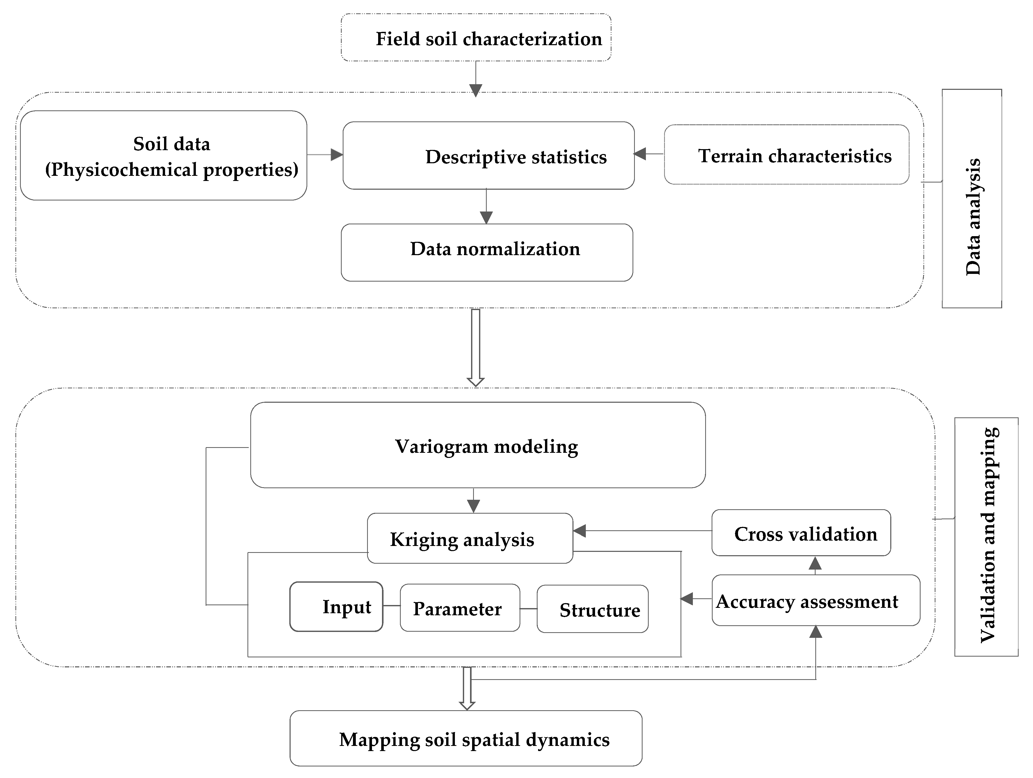
2. Materials and Methods

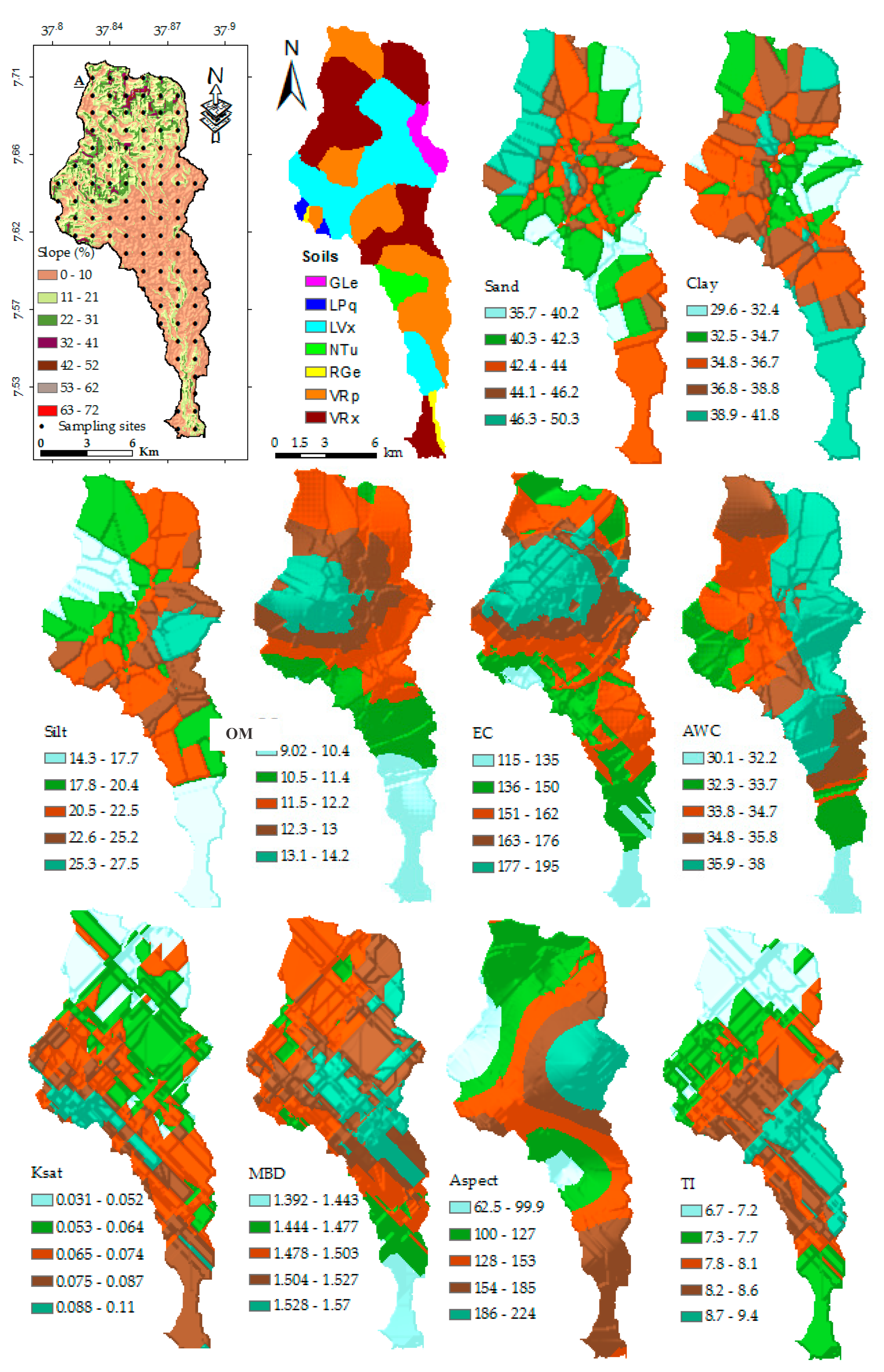
2.1. Site Description

The study area is a 117 km² rural watershed located in the mountainous part of Rift Valley Lakes basin (Figure 1) between 7°30′ and 7°43′N, and 37°48′ and 37°54′E. The region is typified by steep-to-moderate hill slopes signified by two distinct features: rugged mountainous areas in the North and Northwest part of the watershed and lowlands in the eastern most part of the watershed. The climate in the area is mainly controlled by seasonal migration of the Inter-Tropical Convergence Zone and its associated atmospheric circulation [32]. The mean annual rainfall lies between 1280 and 1339 mm and the mean annual temperature in Hosanna station varies from 11 to 22 °C in the watershed.

Based on the 2018 Landsat based land cover classification, the dominant land use in the area were agricultural (48.4%) and bushland units (45.2%). Grazing land, mixed forest and water body covered the remaining 6.4%. Landscape datasets employed in the study included spatial soil attributes and elevation data with 30 m horizontal and 1 m vertical resolution [33].

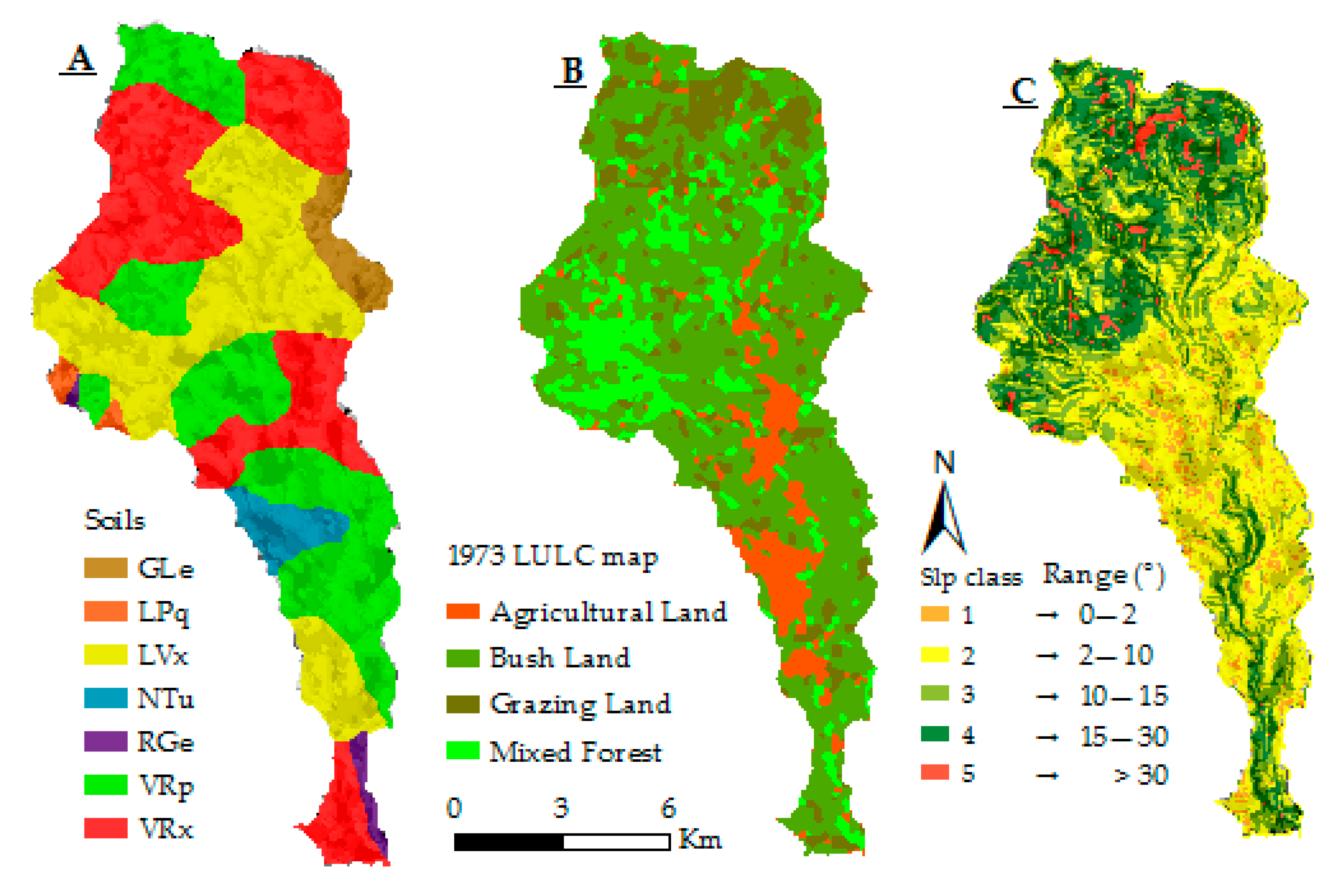
2.2. Soil Survey and Mapping

A combination of field and laboratory work intended to identify the basic physicochemical properties of soils, establish the distribution of those soils at specific map scales, and interpret the information for a variety of uses. Soil samples were collected in a grid scheme field observation (approximately 1 sample for each 1 km² grid) that uses soil sample pits and description augers (see Section 3.1). The sampling sites were selected on an arable area (117 km²) in Southwestern Ethiopia, where agricultural fields and bush cover are the dominant land uses. Projected coordinates (UTM) for each soil sample were recorded to help soil property spatial characterization.

The field soil survey followed the latest United States Department of Agriculture (USDA)—natural resource conservation service norms and standards for field mapping [34]. Soil sampling allowed the estimation and characterization of soil physical and chemical attributes at unsampled sites through existing models. Because of the high complexity relationships among soil properties and the unpredictable spatial pattern [35], the deterministic method of soil characterization does not result in accurate estimation. Probabilistic methods, on the other hand, admit some uncertainty about how soil properties could vary in space, and soil properties at the unmeasured sites are considered to be outcomes of some random process [36].

The sub-horizontal structure [37] indicated the existence of varying soil landscape relationships and that the vertical position and horizontal location of each layer could be derived from the elevation above sea level using the digital elevation model. The surface was built using Kriging point iteration, a model suitable to analyze datasets with a spatial autocorrelation. Kriging estimates the statistical relationships among the sample points with the assumption that the distance between sampling points reflects a spatial correlation that can be used to explain data variations [38]. The algorithm implemented for the Kriging model first creates an empirical semivariogram representing the variance for each pair of observation points followed by adjustment of the model to fit the semivariogram (see Section 2.3). The methodology adopted in this study is presented in the following flowchart (Figure 2).

Spatial Mapping of Topography Index

The standard topographic index (TI) within the yopographic hydrologic model (TOPMODEL) (Equation (1)) uses the catchment digital elevation model. The soil–topographic wetness index analysis (Equation (2)), on the other hand, extends the purely topography-based TOPMODEL analysis by accounting for spatial variation in hydrologically relevant soil properties [39]. TOPMODEL concepts are generalized in a semi-physical representation of rainfall-runoff dynamics, which is parameterized with catchment topographic data and initial conditions of soil moisture. The topographic index components in the model indicate that as the subsurface contributing area increases, there is a likelihood increase in the relative saturation. In addition, the TI incorporates Darcy’s law to estimate subsurface flow proportionality with the hydraulic gradient approximated by the tangent of the ground-surface slope (tan β). A steep topographic slope makes a greater hydraulic gradient and increases drainage potential, which, in turn, reduces the level of saturation. The topographic index (TI) within TOPMODEL is expressed as

$$TI=\ln (\frac{\alpha }{\tan \beta })$$

(1)

$$STWI=\ln (\frac{\alpha }{\mathrm{T} \tan \beta })$$

(2)

where α is the upslope contributing area for the cell per unit of contour line (m), tan β is the topographic slope of the cell, and T is the transmissivity (soil depth × saturated soil hydraulic conductivity) of the uppermost layer of soil (m² d⁻¹) [40,41].

2.3. Geostatistical Analysis

A geostatistical analysis was conducted to elucidate the spatial patterns of soil variability within the study area and to allow the interpolation of soil variables to unmeasured locations. Unsampled soil properties across the entire spatial domain were produced using the variogram model in kriging. Variogram modeling is an advanced geostatistical procedure that generates an estimated surface from a scattered set of points with z-values. Prediction maps were created using a set of training data to employ Kriging point iteration. Kriging works with the regionalized variable theory [42,43], assuming that the spatial variation in the phenomenon represented by the z-values is statistically homogeneous. The spatial variation is quantified using semivariogram [44] computed from soil samples collected from field and laboratory datasets across the watershed following a gridded sampling scheme (Figure 3). Omnidirectional experimental semi-variograms that quantify the dissimilarity γ(h) between observations as a function of the separation distance h were computed in ArcGIS 10.6.1 as half the average squared difference between the components of every data pair. The sample semivariogram for a separation distance of h, lag, is the average squared difference in z-value between pairs of input sample points separated by h. Given n measurements of a spatial attribute (as in Equation (3)), the method of moments estimate of the semi-variogram is calculated as

$$\gamma \left(h\right)= \frac{1}{2\left|N\left(h\right)\right| }{\displaystyle \sum }_{N\left(h\right)}\left(Z\left(x_i\right)-Z\left(x_i\right){)}^2\right)$$

(3)

where N(h) ≡ (x_i, x_j)}: x_i − x_j = h; i, j = 1, 2, …, n is the set of all pairs of samples located a vector distance h apart, and N(h) is the number of distinct pairs in N(h).

Sill variance depicting the total variance of the process is the maximum value reached by the variogram after an initial increase [26]. The range in geostatistical analysis is the distance at which the variogram reaches the sill, beyond which the process is no longer spatially correlated. The combination of measurement error and variation over distances less than the shortest sampling interval is explained by the nugget variance at lag distance 0 [45]. High variations in nugget indicate high, unquantified, fine-scale variability and measurement error. On the other hand, the spatial heterogeneity of soil property dynamics is explained by the sill value [46]. During data analysis, the distribution of soil properties was assessed using an exploratory data analysis employing the Kolmogorov–Smirnov test.

3. Results and Discussion

3.1. Soil Spatial Analysis, Classification, and Mapping

Table 1. Ranking qualifiers in reference soil groups and soil types in the study area.

Qualifiers
1* Formative a		2 Intergrade		1 Strong Expression		Secondary Characteristics			5 Haplic e	6 Prefix f
						3 (Horizon, Property & Material)		4 Other
Qualifier	RSGs	Qualifier	Intergrade To	Qualifier	RSG	Qualifierb	DRc	Qualifierd	Haplic
Chromic	Luvisols	Luvic	Luvisols	Hyperchromic	Luvisols	Profondic	Argic horizon	Chromic	Haplic	Epihyper
Humic	Nitisols	Nitic	Nitisols	Nitic	Nitisols	Nitic	Nutic horizon	Rhodic	Haplic	Hypohumic
Anthropic	Regosols	Regic	Regosols	Umbric	Regosols	Umbric	Ochric horizon	Anthropic	Haplic	Paraanthropic
Leptic	Leptosols	Leptic	Leptosols	Lithic	Leptosols	Leptic	rugged topography elevated Soils	Skeletic	Haplic	Paralithic
Gleyic	Gleysols	Gleyic	Gleysols	Gleyic	Gleysols	Endogleyic	Water logging by shallow GW	Acidic	Haplic	Hypoacidic
Chromic	Vertisols	Vertic	Vertisols	Parachromic	Vertisols	Vertic	Granular self-mulching	Chromic	Haplic	Hypochromic
Pellic	Vertisols	Vertic	Vertisols	Orthipellic	Vertisols	Vertic	Granular self-mulching	Pellic	Haplic	Epipellic

Note: ^{1*, 1, 2, 3, 4, 5} suggestions for ranking qualifiers in soil unit names for the most common qualifiers. ⁶ names of reference soil groups can further be explained using prefixes added with formative element qualifiers. ^a influential and shaping qualifier elements for naming reference soil groups units. ^b referring to diagnostic horizons, properties or soil materials. ^c directly related diagnostic horizon, property or soil material. ^d secondary characteristics qualifiers referring to soil characteristics that indicates a particular water regime, soil solution or groundwater chemistry, exchange complex specification, weak soil development or morphological characteristics than diagnostic horizons, properties or soil materials. ^e having the typical expression of the reference soil group in the sense that there is no further or meaningful characterisation. ^f indicates depth of occurrence or degree of expression of soil characteristics. RSGs indicate reference soil groups.

shows the ranking of qualifiers [34] based on the Food and agricultural organization reference soil group guideline [37]. Following the field soil survey, a laboratory analysis and descriptive augers, seven soil taxa at the family level of USDA soil taxonomy hierarchy were identified and mapped. These soil types were chromic luvisol, chromic vertisol, haplic gleysol, humic nitisol, lithic leptosol, ochric regosol, and pellic vertisols (Figure 3). Nearly 92% of the catchment was covered with three soil types: chromic vertisol (33.3%), chromic luvisol (30.2%) and pellic vertisol (28.2%). The remaining soil classes (humic nitisol, haplic gleysol, lithic leptosol, and ochric regosol) covered 8% of the area.

3.2. Soil Wetness and Dryness with Topography

In order to assess the spatial variability of terrain elevation with soil wetness/dryness, the soil topographic wetness index, a map, Figure S1E, was developed from the coincidence of TI (Figure S1B) and soil type (Figure S1D). Reconceptualization of the TI map into the soil topographic wetness index and topographic wetness index provides accurate information on how land use changes with terrain and soil wetness/dryness at the lowest functional units. The watershed topographic wetness index was lumped into 10 equal area intervals ranging from 1 to 10, with index class 1 covering 10% of the watershed area with the lowest topographic wetness index (i.e., lowest propensity to saturate) and index class 10 containing 10% of the watershed with the highest topographic wetness index (i.e., highest propensity to saturate). Pertinent soil information was extracted with an aerially weighted soil topographic wetness index and included in the index input table by soil wetness class. The results show that the saturated hydraulic conductivity (Ksat) of soils has an unpredictable pattern with elevation.

3.3. Soil Topography Relationships

For each soil sample, texture was defined using sand and clay content obtained from a laboratory analysis and using soil-plant-air-water (SPAW) soil water characteristics’ pedo-transfer functions. During the textural classification, SPAW soil water characteristic equations [47,48] are valid within a range of approximately 0%–60% clay content and 0%–95% sand content. In addition, the spatial relationships between soil properties and topographic attributes for the data points were assessed for the first and second soil layers. In each sampling point, average topographic height, slope and aspect were calculated from the digital elevation model in ArcGIS environment. The spatial dependence of each individual variable as well as the relationship between them was evaluated with Pearson correlation and descriptive statistics of soil topography variables.

The descriptive statistical results for altitude and soil physical attributes are presented in

Table 2. Descriptive statistics for topographic and soil variables in Batena Watershed, first layer.

	TI	Depth (m)	Sand (%)	Clay (%)	Silt (%)	OM	EC	MBD	AWC	KSat	Slope%	Aspect	Elevation
Mean	7.97	0.34	42.23	37.69	20.07	11.17	148.9	1.50	34.6	0.07	11.5	147.4	2434.03
SE	0.53	0.03	2.95	2.78	2.51	0.52	11	0.03	1.2	0.02	1.25	15.7	32.37
Median	6.95	0.32	42	36	17.5	10.71	148.5	1.51	33.5	0.02	10.14	137.0	2395
Mode	6.95	0.35	38	34	9	10.71	163.2	1.56	41.7	0.01	3.73	105.85	2311
CV	2.95	0.17	16.40	15.50	13.97	2.89	61	0.16	6.6	0.09	6.97	87.4	180.21
Kurtosis	3.23	6.37	0.08	−0.98	0.28	0.61	1.04	0.15	4.5	1.24	1.94	−0.78	0.25
Skewness	2.02	2.01	0.01	0.30	0.68	0.02	0.64	0.18	0.98	1.50	1.29	0.27	0.50
Minimum	5.66	0.1	8	13.5	0.5	3.71	41.4	1.15	18	0.01	2.12	1.36	2088
Maximum	16.64	1	76	65	52	17.02	321	1.87	57.5	0.35	32.97	322.5	2871
CL (95.0%)	1.08	6.32	6.02	5.69	5.12	1.06	22.37	0.06	2.43	0.03	2.56	32.06	66.10

Note: CV, CL, SE and SD denotes the coefficient of variation, 95% confidence level, the standard error, and sample standard deviation, respectively. OM, EC, MBD, AWC, and Ksat represent soil organic matter, electrical conductivity, moist bulk density, and saturated hydraulic conductivity, respectively.

and

Table 3. Second layer descriptive statistics for topographic and soil variables in the study area.

	TI	Depth	Sand (%)	Clay (%)	Silt (%)	OM	EC	MBD	AWC	Slope	Elevation
Mean	5.56	0.36	23.24	51.59	25.17	10.06	137.43	1.51	35.30	12.00	2424.59
SE	0.58	0.03	3.70	3.54	2.55	0.54	9.02	0.03	2.41	1.37	29.96
Median	5	0.36	16.5	52	24	9.71	131.1	1.52	34.57	10.31	2395
Mode	7	0.36	16	52	32	13.80	135.7	1.56	32.03	3.73	2311
CV	3.03	0.13	19.25	18.41	13.26	2.79	46.87	0.14	12.50	7.10	155.70
Kurtosis	−1.22	−0.83	0.71	−0.58	0.24	0.54	0.34	0.13	16.03	1.80	0.25
Skewness	0.08	0.23	1.15	−0.58	0.49	0.48	0.62	0.44	3.37	1.31	0.49
Minimum	1	0.11	0	15	1	4.92	48.9	1.28	14.86	3.33	2088
Maximum	10	0.61	75	79	58	17.02	254.1	1.87	90.87	32.97	2785
CL (95.0%)	1.20	0.05	7.61	7.28	5.25	1.10	18.54	0.06	4.94	2.81	61.59

. Samples were collected along the slope with altitude values ranging from 2065 to 2950 m above sea level. Frequency distribution was evaluated for these attributes and the results are summarized in Table 2 and Table 3. According to Webster [35], skewness values up to 0.5 suggest a specific attribute with normal distribution. Besides altimetry, the only attributes that showed both features, a skewness smaller than 0.5 and a normal distribution were sand, clay, OM, and soil bulk density. Negative skewness values (Table 3) indicate data that are skewed to the left, which means that the left tail is long relative to the right tail. On the other hand, positive skewness values indicate data that are skewed right. The kurtosis shows how the tails of a distribution differ from the normal distribution. Negative kurtosis (Table 2 and Table 3) indicates a distribution flatter than a normal curve and tails that are heavier than a normal distribution are indicated by positive kurtosis values. The small standard deviation values (<30%) were found for most of the variables, other than elevation and aspect. The high values of coefficient of variation for elevation can be explained by the great amplitude of variation in the area (minimum and maximum values).

The summary statistics for the second soil layer indicate that topographic and soil properties are highly variable between sampling points in the watershsed.

The spatial dependence of each individual variable was evaluated with semivariogram and cross semivariograms (Figure 4). The unsampled estimates of variables across the entire spatial domain were produced using the variogram model in kriging. The spatial variation was quantified by the semivariogram estimated by using the sample semivariogram computed from point input dataset. Figure 4 summarizes the experimental semi-variogram plots and how to relate the practical semi-variogram to the ideal models. It can be seen that whilst some variables may follow simple behaviour (e.g., elevation), many others, such as sand, clay, silt, moist bulk density, available water content, organic matter, electrical conductivity, and saturated hydraulic conductivity, may require a non-linear or relatively complex models to describe the experimental semi-variogram.

There are several important features to note from the sample semivariogram plots. For some variables, at relatively short lag distances of h, the semivariance is small but increases with the distance between the pairs of sample points. At a distance referred to as the range, the semivariance levels off to a relatively constant value referred to as the sill. This implies that beyond this range distance, the variation in z-values is no longer spatially correlated. Within the range, the z-value variation is smaller when the pairs of sample points are closer together. The extent of the x-axis of the semivariogram is determined by the distance between the most widely separated pair of points in the input sample data.

The results show that there was a spatial correlation between slope, sand, silt, clay, AWC, EC, OM, and MBD. A positive correlation was characterized between soil depth and AWC, EC and sand content, OM and EC, AWC and OM, and Ksat and soil depth (

Table 4. Top layer descriptive statistics: Pearson product moment correlation for soil-topography variables.

Note: TI, OM, EC, MBD, AWC, and Ksat represent topographic index, soil organic matter, electrical conductivity, moist bulk density, and saturated hydraulic conductivity, respectively.

). For the second soil layer (

Table 5. Geo-statistical correlation for second layer soil-topography variables.

), a positive correlation was characterized between TI and silt content, soil depth and EC, sand content and depth, clay content and TI, sand content and OM, EC and soil depth, and clay content and MBD. In addition, AWC and MBD, slope and elevation, soil depth and terrain elevation, and AWC and clay content were positively correlated. A low positive and negative relation was reported between the other variables.

In summary, Pearson product moment correlation (Table 4 and Table 5) better estimates the linear relationship between two variables. In order to assess the linearity and stationarity of the dataset, Pearson correlation was also calculated for the log-transformed data (Table 4 and Table 5). We also believe that any two variables may not linearly relate to each other to implement Pearson correlation. As a result, the monotonic relationship between two variables was assessed using Spearman’s rank correlation coefficient (or Spearman’s rho) and Kendall’s rank correlation coefficient (or Kendall’s tau) [49]. For a detailed presentation of a statistical test comparison between Pearson correlation, Spearman’s rho, and Kendall’s tau, please see the Excel Supplementary File (Tables S1 and S2).

Pearson correlation being the most used statistical tool to evaluate the relationship between two variables, the coefficient of correlation is also used in geostatistics to improve data interpolation. The correlation between the soil-topography index and selected soil physicochemical properties for top and second layers is presented in Figure 5.

The graph relating topographic index (TI) with soil physicochemical properties indicated that soil organic matter (OM), moist bulk density (MBD), slope, depth, and saturated hydraulic conductivity (K_sat) shows a decrease in TI for both soil layers. However, the sand content in the upper and second soil layers shows a relatively different trend of a tendency for a slight increase for the first soil layer, while a noticeable decrease is observed for the second soil layer. On the other hand, silt and clay contents, OM, OC, and available water content (AWC) show an increase with TI.

For the first soil layer, the correlation coefficients (r) between TI and silt, sand, clay contents were 0.36, 0.55, and 0.71, respectively. The ‘r’ values between TI and other soil and topography variables such as OM, EC, MBD, slope, K_sat, and AWC were 0.66, 0.49, 0.32, 0.65, 0.66, and, 0.35, respectively (Figure 5, upper panel).

In the second soil layer, the increase in the TI resulted in an increase in clay and AWC with a relatively stronger correlation coefficient of 0.6 and 0.66, respectively (Figure 5, lower panel). On the contrary, the influence of TI on the silt content was relatively weaker (r = 0.36). Linear regression also indicated that the correlation between Ksat and MBD with TI is 0.66 and 0.37, respectively.

3.4. Soil, Topography and Land Use Relationships

Soil–land use–slope relationships and the spatial variability of land use units can be collated based on six snapshots (1973–2018) for five slope classes. For example, in 1973 (Figure 6, Table S3), 141 ha of the agricultural area was topographically located in slope class 2 (slope ranging from 2 to 10°) and the specific soil type was chromic vertisol.

As an important indicator of topography, terrain slope has a substantial effect on land use, thereby affecting soil fertility and the density and pattern of land use. It was also indicated that time series land use change pattern changed in agriculturally accessible and arable soils (Table S3), while showing a relative stability in mountainous and poorly fertile soils. According to World Food and Agricultural Organization study [37], soils such as vertisols, luvisols, nitisols, and gleysols are fertile soils. On the other hand, leptosols and regosols are weakly developed mineral soils that are extensive in eroding lands, arid and semi-arid areas and mountain regions. Intensification of agricultural practices leading to a decrease in soil fertility could also be related to the acute shortage of land on the gentle slope.

Studies [50,51] highlighted that in line with agricultural unsuitability, properties of dryness/wetness and magnitude and seasonal pattern of rainfall alter the pattern land use change and soil fertility. This suggests that management for any one of these soil properties may yield unintended cascading effects throughout the soil subsystem.

Slope Effects on Soil Physicochemical Properties and Land Cover Distribution

Slope has a significant effect on the intensity of soil erosion, which can affect soil fertility and patterns of land use. Balba [52] indicated that steep slopes are typified by rapid runoff, less moisture entering the soil, and lower crop productivity. To evaluate the impact of slope position on soil texture (i.e., sand, clay, and silt), OM, and AWC, the spatial variation of each variable is presented in Table S4 (Excel Supplementary File). Figure 7 illustrates the spatial relation between catchment slope and selected soil physicochemical properties. The change in OM and AWC is highly related to the type of soil and land cover density. For instance, a highly leached leptosol is characterized by low OM.

Other similar studies conducted in the Ethiopian highlands [53] indicated that variations in soil physicochemical properties are related to slope position and land use. According to their findings, low soil pH was observed at forested areas in the upslope position, which was characterized by high OM. They also noted that high pH values were recorded on lower slope positions where low OM cultivation land was the dominant land use. Griffiths et al. [54], highlighted that topography could influence soil physicochemical properties, such as OM, soil depth, and texture. Our findings agree with Hu et al. [55], who showed that a decrease in OM and the associated changes in soil nutrients were related to land use conversions into agriculture and increased incidence of tillage.

Details of topography effects on soil physicochemical properties and land cover distribution are presented in Table S4 (excel supplementary file). It is shown that land use was significantly affected by slope position, soil type, and soil fertility. For illustration, in 2018, 35.5 ha of the agricultural area was located in slope class 2 (slope ranging from 2 to 10°) in a clayey soil type 2 (i.e., abundance between 34.7% and 38.1%).

4. Conclusions

In areas with heterogeneous topography, soil is spatially variable and the way we manage catchment soil and land use alters the fluxes of water and sediment. This effect is more pronounced in highly rugged agrarian landscapes where there is a significant land disturbance and topographic influences are dominant. In this regard, knowledge of soil properties associated with topographical attributes is vital for modelling soil–landscape relationships and establishing sustainable on-field management practices. To this end, previous studies on the spatial variability of soil properties have either been site-specific, coarse in scale, or implemented pedo-transfer-functions that neither accounted for environmental effects nor provided all the required data inputs.

In this study, we assessed soil–landscape relation and mapped soil property spatial dynamics to understand landscape physicochemical processes and used the result for hydrological modelling and future soil and watershed management applications. The significance of the work therefore stems from the fact that we did not rely on our research using either coarse resolution FAO-soils that assigns the same soil property at different landscape gradient or site-specific and unreliable PTfs. Instead, we developed a soil-landscape relation for a tropical catchment in the Rift Valley basin where data are a scarce resource.

The relationship between topography and the spatial variability of soil physicochemical properties was evaluated using Kriging predictions and it is shown that the use of Kriging is a promising tool in soil physics. Descriptive statistics were used to evaluate central tendency and to explore the correlation between spatially explicit soil and terrain attributes. In an study aiming to relate practical semivariogram to the ideal models, it is seen that whilst some variables may follow simple behaviour (e.g., elevation), many others, such as sand, clay, silt, moist bulk density, available water content, organic matter, electrical conductivity, and saturated hydraulic conductivity may require relatively complex models to describe the experimental semi-variogram.

References

1. Jiang, S.-H.; Huang, J.; Yao, C.; Yang, J. Quantitative risk assessment of slope failure in 2-D spatially variable soils by limit equilibrium method. Appl. Math. Model. 2017, 47, 710–725. [Google Scholar] [CrossRef]
2. Jiang, S.-H.; Huang, J.-S. Efficient slope reliability analysis at low-probability levels in spatially variable soils. Comput. Geotech. 2016, 75, 18–27. [Google Scholar] [CrossRef]
3. Kreznor, W.R.; Olson, K.R.; Banwart, W.L.; Johnson, D.L. Soil, landscape, and erosion relationships in a northwest Illinois watershed. Soil Sci. Soc. Am. J. 1989, 53, 1763–1771. [Google Scholar] [CrossRef]
4. Ayele, G.T.; Tebeje, A.K.; Demissie, S.S.; Belete, M.A.; Jemberrie, M.A.; Teshome, W.M.; Mengistu, D.T.; Teshale, E.Z. Time Series Land Cover Mapping and Change Detection Analysis Using Geographic Information System and Remote Sensing, Northern Ethiopia. Air Soil Water Res 2018, 11. [Google Scholar] [CrossRef] [Green Version]
5. Asres, R.S.; Tilahun, S.A.; Ayele, G.T.; Melesse, A.M. Analyses of Land Use/Land Cover Change Dynamics in the Upland Watersheds of Upper Blue Nile Basin. Spring Geogr 2016. [Google Scholar] [CrossRef]
6. Ceddia, M.B.; Vieira, S.R.; Villela, A.L.O.; Mota, L.D.S.; Anjos, L.H.C.D.; Carvalho, D.F.D. Topography and spatial variability of soil physical properties. Sci. Agric. 2009, 66, 338–352. [Google Scholar] [CrossRef] [Green Version]
7. WeillA, M.; VieiraB, S.; SparovekC, G. Assessment of the spatial relationship between soil properties and topography over a landscape. In Proceedings of the 19th World Congress of Soil Science, Soil Solutions for a Changing World, Brisbane, Australia, 1–6 August 2010; pp. 20–23. [Google Scholar]
8. Vauclin, M.; Vieira, S.; Vachaud, G.; Nielsen, D. The Use of Cokriging with Limited Field Soil Observations 1. Soil Sci. Soc. Am. J. 1983, 47, 175–184. [Google Scholar] [CrossRef]
9. Saxton, K.E.; Rawls, W.J. Soil water characteristic estimates by texture and organic matter for hydrologic solutions. Soil Sci. Soc. Am. J. 2006, 70, 1569–1578. [Google Scholar] [CrossRef] [Green Version]
10. Cosby, B.; Hornberger, G.; Clapp, R.; Ginn, T. A statistical exploration of the relationships of soil moisture characteristics to the physical properties of soils. Water Resour. Res. 1984, 20, 682–690. [Google Scholar] [CrossRef] [Green Version]
11. Rawls, W.; Brakensiek, D. Estimation of soil water retention and hydraulic properties. In Unsaturated Flow in Hydrologic Modeling; Springer: Berlin, Germany, 1989; pp. 275–300. [Google Scholar]
12. Wösten, J.; Lilly, A.; Nemes, A.; Le Bas, C. Development and use of a database of hydraulic properties of European soils. Geoderma 1999, 90, 169–185. [Google Scholar] [CrossRef]
13. Abdelbaki, A.M.; Youssef, M.A.; Naguib, E.M.; Kiwan, M.E.; El-giddawy, E.I. Evaluation of pedotransfer functions for predicting saturated hydraulic conductivity for US soils. In Proceedings of the 2009, Reno, NV, USA, 21–24 June 2009; p. 1. [Google Scholar]
14. Harrison, K.W.; Kumar, S.V.; Peters-Lidard, C.D.; Santanello, J.A. Quantifying the change in soil moisture modeling uncertainty from remote sensing observations using Bayesian inference techniques. Water Resour. Res. 2012, 48, 11. [Google Scholar] [CrossRef]
15. Gijsman, A.; Jagtap, S.; Jones, J. Wading through a swamp of complete confusion: How to choose a method for estimating soil water retention parameters for crop models. Eur. J. Agron. 2002, 18, 77–106. [Google Scholar] [CrossRef]
16. Luo, Y.; Yang, S.; Zhao, C.; Liu, X.; Liu, C.; Wu, L.; Zhao, H.; Zhang, Y. The effect of environmental factors on spatial variability in land use change in the high-sediment region of China’s Loess Plateau. J. Geogr. Sci. 2014, 24, 802–814. [Google Scholar] [CrossRef] [Green Version]
17. Ayele, G.T.; Demissie, S.S.; Tilahun, S.A.; Jeong, J.; Jemberie, M.A. Assessing drought severity from multi-temporal GIMMSNDVI and rainfall interactions. In Proceedings of the 36th Hydrology and Water Resources Symposium: The art and science of water, Barton, Australia, 2015; p. 306. [Google Scholar]
18. O’Geen, A. Soil water dynamics. Nat. Educ. Knowl. 2012, 3, 12. [Google Scholar]
19. Quan, B.; Römkens, M.; Li, R.; Wang, F.; Chen, J. Effect of land use and land cover change on soil erosion and the spatio-temporal variation in Liupan Mountain Region, southern Ningxia, China. Front. Environ. Sci. Eng. China 2011, 5, 564–572. [Google Scholar] [CrossRef]
20. Opršal, Z.; Šarapatka, B.; Kladivo, P. Land-use changes and their relationships to selected landscape parameters in three cadastral areas in Moravia (Czech Republic). Morav. Geogr. Rep. 2013, 21, 41–50. [Google Scholar] [CrossRef] [Green Version]
21. Ayele, G.T.; Demessie, S.S.; Mengistu, K.T.; Tilahun, S.A.; Melesse, A.M. Multitemporal Land Use/Land Cover Change Detection for the Batena Watershed, Rift Valley Lakes Basin, Ethiopia. Spring Geogr 2016. [Google Scholar] [CrossRef] [Green Version]
22. Pachepsky, Y.A.; Timlin, D.; Rawls, W. Soil water retention as related to topographic variables. Soil Sci. Soc. Am. J. 2001, 65, 1787–1795. [Google Scholar] [CrossRef]
23. Rezaei, S.A.; Gilkes, R.J. The effects of landscape attributes and plant community on soil chemical properties in rangelands. Geoderma 2005, 125, 167–176. [Google Scholar] [CrossRef]
24. Quesada, C.; Lloyd, J.; Schwarz, M.; Baker, T.; Phillips, O.L.; Patiño, S.; Czimczik, C.; Hodnett, M.; Herrera, R.; Arneth, A. Regional and large-scale patterns in Amazon forest structure and function are mediated by variations in soil physical and chemical properties. Biogeosci. Discuss. 2009, 6, 3993–4057. [Google Scholar] [CrossRef] [Green Version]
25. Entwistle, J.A.; Abrahams, P.W.; Dodgshon, R.A. The geoarchaeological significance and spatial variability of a range of physical and chemical soil properties from a former habitation site, Isle of Skye. J. Archaeol Sci. 2000, 27, 287–303. [Google Scholar] [CrossRef]
26. Glendell, M.; Granger, S.J.; Bol, R.; Brazier, R.E. Quantifying the spatial variability of soil physical and chemical properties in relation to mitigation of diffuse water pollution. Geoderma 2014, 214, 25–41. [Google Scholar] [CrossRef] [Green Version]
27. Sidorova, V.A.; Krasilnikov, P.V. Soil-geographic interpretation of spatial variability in the chemical and physical properties of topsoil horizons in the steppe zone. Eurasian Soil Sci. 2007, 40, 1042–1051. [Google Scholar] [CrossRef]
28. Nicolau, R.F.; Mercante, E.; Maggi, M.F.; de Souza, E.G.; Gasparin, E. Spatial variability of soil chemical attributes and productivity and the chemical and physical properties of oranges. Cienc. Investig. Agrar. 2014, 41, 337–347. [Google Scholar] [CrossRef] [Green Version]
29. Wani, M.A.; Shaista, N.; Wani, Z.M. Spatial Variability of Some Chemical and Physical Soil Properties in Bandipora District of Lesser Himalayas. J. Indian Soc. Remote 2017, 45, 611–620. [Google Scholar] [CrossRef]
30. Mora-Vallejo, A.; Claessens, L.; Stoorvogel, J.; Heuvelink, G.B. Small scale digital soil mapping in Southeastern Kenya. Catena 2008, 76, 44–53. [Google Scholar] [CrossRef]
31. Cianfrani, C.; Buri, A.; Verrecchia, E.; Guisan, A. Generalizing soil properties in geographic space: Approaches used and ways forward. PLoS ONE 2018, 13, e0208823. [Google Scholar] [CrossRef] [Green Version]
32. Ayele, G.T.; Teshale, E.Z.; Yu, B.F.; Rutherfurd, I.D.; Jeong, J. Streamflow and Sediment Yield Prediction for Watershed Prioritization in the Upper Blue Nile River Basin, Ethiopia. Water 2017, 9, 782. [Google Scholar] [CrossRef] [Green Version]
33. Thompson, J.A.; Bell, J.C.; Butler, C.A. Digital elevation model resolution: Effects on terrain attribute calculation and quantitative soil-landscape modeling. Geoderma 2001, 100, 67–89. [Google Scholar] [CrossRef]
34. USDA, S.T. A Basic System of Soil Classification for Making and Interpreting Soil Surveys. In USDA Pittsburgh; 1999. Available online: https://www.nrcs.usda.gov/wps/portal/nrcs/main/soils/survey/class/taxonomy/ (accessed on 5 March 2019).
35. Webster, R. Is soil variation random? Geoderma 2000, 97, 149–163. [Google Scholar] [CrossRef]
36. Isaaks, E.H.; Srivastava, R.M. Applied Geostatistics; Oxford University Press: New York, NY, USA, 1989; p. 561. [Google Scholar]
37. Spaargaren, O.C.; Deckers, J. The world reference base for soil resources. In Soils of Tropical Forest Ecosystems; Springer: Berlin, Germany, 1998; pp. 21–28. [Google Scholar]
38. Laurent, F.; Poccard-Chapuis, R.; Plassin, S.; Pimentel Martinez, G. Soil texture derived from topography in North-eastern Amazonia. J. Maps 2017, 13, 109–115. [Google Scholar] [CrossRef]
39. Beven, K. Runoff production and flood frequency in catchments of order n: An alternative approach. In Scale Problems in Hydrology; Springer: Berlin, Germany, 1986; pp. 107–131. [Google Scholar]
40. Easton, Z.M.; Fuka, D.R.; Walter, M.T.; Cowan, D.M.; Schneiderman, E.M.; Steenhuis, T.S. Re-conceptualizing the soil and water assessment tool (SWAT) model to predict runoff from variable source areas. J. Hydrol. 2008, 348, 279–291. [Google Scholar] [CrossRef]
41. Schneiderman, E.M.; Steenhuis, T.S.; Thongs, D.J.; Easton, Z.M.; Zion, M.S.; Neal, A.L.; Mendoza, G.F.; Todd Walter, M. Incorporating variable source area hydrology into a curve-number-based watershed model. Hydrol. Process. Int. J. 2007, 21, 3420–3430. [Google Scholar] [CrossRef]
42. Coburn, T.C. Geostatistics for Natural Resources Evaluation; Taylor & Francis: Abingdon-on-Thames, UK, 2000. [Google Scholar]
43. Morgan, C.J. Theoretical and practical aspects of variography. In Particular, Estimation and Modelling of Semi-Variograms over Areas of Limited and Clustered or Widely Spaced Data in A Two-Dimensional South African Gold Mining Context; WIReDSpace: South Africa, 2011. [Google Scholar]
44. McBratney, A.; Webster, R. Choosing functions for semi-variograms of soil properties and fitting them to sampling estimates. J. Soil Sci. 1986, 37, 617–639. [Google Scholar] [CrossRef]
45. Webster, R.; Oliver, M.A. Geostatistics for Environmental Scientists; John Wiley & Sons: Hoboken, NJ, USA, 2007. [Google Scholar]
46. Bruland, G.L.; Grunwald, S.; Osborne, T.Z.; Reddy, K.R.; Newman, S. Spatial distribution of soil properties in Water Conservation Area 3 of the Everglades. Soil Sci. Soc. Am. J. 2006, 70, 1662–1676. [Google Scholar] [CrossRef] [Green Version]
47. Saxton, K.; Rawls, W.J.; Romberger, J.; Papendick, R. Estimating generalized soil-water characteristics from texture 1. Soil Sci. Soc. Am. J. 1986, 50, 1031–1036. [Google Scholar] [CrossRef]
48. Saxton, K.E.; Willey, P.H.; Rawls, W.J. Field and pond hydrologic analyses with the SPAW model. In Proceedings of the 2006 ASAE Annual Meeting, Boston, MA, USA, 19–22 August 2006; p. 1. [Google Scholar]
49. Chok, N.S. Pearson’s Versus Spearman’s and Kendall’s Correlation Coefficients for Continuous Data. Master’s Thesis, University of Pittsburgh, Pittsburgh, PA, USA, 2010. [Google Scholar]
50. Jemberie, M.A.; Awass, A.A.; Melesse, A.M.; Ayele, G.T.; Demissie, S.S. Seasonal Rainfall-Runoff Variability Analysis, Lake Tana Sub-Basin, Upper Blue Nile Basin, Ethiopia. Spring Geogr. 2016. [Google Scholar] [CrossRef]
51. Seka, A.M.; Awass, A.A.; Melesse, A.M.; Ayele, G.T.; Demissie, S.S. Evaluation of the Effects of Water Harvesting on Downstream Water Availability Using SWAT. Spring Geogr 2016, 763–787. [Google Scholar] [CrossRef]
52. Balba, A.M. Management of Problem Soils in Arid Ecosystems; CRC Press: Boca Raton, FL, USA, 2018. [Google Scholar]
53. Abate, N.; Kibret, K. Effects of land use, soil depth and topography on soil physicochemical properties along the toposequence at the Wadla Delanta Massif, Northcentral Highlands of Ethiopia. Environ. Pollut. 2016, 5, 2. [Google Scholar] [CrossRef] [Green Version]
54. Griffiths, R.P.; Madritch, M.D.; Swanson, A.K. The effects of topography on forest soil characteristics in the Oregon Cascade Mountains (USA): Implications for the effects of climate change on soil properties. For. Ecol. Manag. 2009, 257, 1–7. [Google Scholar] [CrossRef]
55. Hu, H.; Ma, H.; Wang, Y.; Xu, H. Influence of land use types to nutrients, organic carbon and organic nitrogen of soil. Soilland Water Conserv. China 2010, 11, 40–42. [Google Scholar]
Figure 1. Location map of the study area: geographical setting with elevation range (left) and Ethiopian river basins (right).
Soilsystems 04 00001 g001
Figure 2. Simplified methodological framework.
Soilsystems 04 00001 g002
Figure 3. Grid scheme soil sampling points on the slope map (left) and catchment soil (right). Note: the soils in the study area were acronymed as gleysols (GLe), lithic leptosols (LPq), chromic luvisols (LVx), humic nitisols (NTu), ochric reghosols (RGe), pellic vertisols (VRp), and chromic vertisols (VRx).
Soilsystems 04 00001 g003
Figure 4. Semivariogram analysis: semivariance in the Y-axis and lag distance or distance between sample points, h (m) in the X-axis. Y-axis values are measures of the spatial dependency between two samples or observations. Curve showing the actual data estimate (black line), model estimate (solid blue line), and predicted variance (blue dotted lines). Laboratory experimental semi-variogram for some of the soil variables showed a sill apparently below the dotted sample variance and well above the dotted sample variance.
Soilsystems 04 00001 g004
Figure 5. Soil-topography regression fit for Y-forecast and topographic index class (X-axis) for top soil layer (upper panel) and topographic index class average representation of soil-topography dynamics in the second soil layer (lower panel).
Soilsystems 04 00001 g005aSoilsystems 04 00001 g005b
Figure 6. Spatial relationship between soil (A), land use (B) and terrain slope (C) in the Batena Watershed. Note: the soils in the study area are acronymed as gleysols (GLe), lithic leptosols (LPq), chromic luvisols (LVx), humic nitisols (NTu), ochric reghosols (RGe), pellic vertisols (VRp), and chromic vertisols (VRx). The 1973 land use and land cover map is presented for illustration purpose. For the remaining time series land use maps, see the soil–land use–slope relationship in Table S3 and Figure S2.
Soilsystems 04 00001 g006
Figure 7. Catchment characteristics: slope and sampling sites, soils, and selected soil physicochemical properties: sand (%), clay (%), silt (%), OM (%), EC (S/m), AWC, Ksat, MBD, Aspect, and TI.
Soilsystems 04 00001 g007