Article

Comparison between Measured and Calculated Thermal Conductivities within Different Grain Size Classes and Their Related Depth Ranges

GeoCentre of Northern Bavaria, Friedrich-Alexander-University Erlangen-Nuremberg, Schlossgarten 5, 91054 Erlangen, Germany
*
Author to whom correspondence should be addressed.
Soil Syst. 2018, 2(3), 50; https://doi.org/10.3390/soilsystems2030050
Submission received: 14 June 2018 / Revised: 23 August 2018 / Accepted: 25 August 2018 / Published: 1 September 2018

Abstract

:
In the field of the efficiency of very shallow geothermal energy systems, there is still a significant need for research activity. To ensure the proper exploitation of this energy resource, the decisive geophysical parameters of soil must be well-known. Within this study, thermal conductivity, as a fundamental property for evaluating the geothermal potential of very shallow geothermal systems, was analyzed and measured with a TK04 device. A dataset, consisting of various geophysical parameters (thermal conductivity, bulk density, water content, and porosity) determined for a large range of different textural soil classes, was collated. In a new approach, the geophysical properties were visualized covering the complete grain size range. The comparison between the measured and calculated thermal conductivity values enabled an investigation with respect to the validity of the different Kersten equations. In the course of this comparison, the influence of effective bulk density was taken into account. In conclusion, both Kersten formulas should be used as recommended and regular bulk density corresponded better to the reference dataset representing the outcomes of the TK04 laboratory measurement. Another objective was to visualize the relation of thermal conductivities within their corresponding textural classes and the validity of Kersten formulas for various bulk densities, depths, and soils. As a result, the accessibility to information for expedient recommendations about the feasibility of very shallow geothermal systems will be improved. Easy, accessible know-how of the fundamentals is important for a growing renewable energy sector where very shallow geothermal installations can also cover heating and cooling demands.

1. Introduction

Due to climate change and the consequent societal rethinking about energy policies in favor of renewable energies, geothermal energy has become progressively important for heating and cooling demands. One critical issue of facing global warming by using geothermal applications is the reduction of emitted greenhouse gases [1,2,3]. To enable proper and sustainable implementation in today’s energy concepts, research into geothermal systems is fundamental. Compared to solar or wind energy, geothermal systems—as part of the renewable energy sector—are not dependent on diurnal varying climatic conditions. These systems are only affected by seasonal temperature changes until a certain depth [4]. Thus, these systems are available at any time and are sustainable if anticipatorily used [5]. Furthermore, low enthalpy geothermal systems can be installed almost everywhere to enable a decentralized energy supply. In vertical shallow geothermal systems (up to 400 m in depth), the thermal conductivity of unconsolidated soil materials only affects the topmost layers. As the contact area between the vertical geothermal systems and the surrounding unconsolidated soil is very small in relation to the total contact area of the whole installed system, the soil’s geothermal potential within the vertical installations is much less decisive. For these geothermal installations, the thermal properties of the underlying bedrock are essential.
In the field of unconsolidated soil, primarily horizontal geothermal systems like collector systems or special forms such as heat baskets come into play to exploit this very shallow geothermal potential (vSGP). The vSGP is defined as the natural thermal potential of unconsolidated soil from the surface down to the bedrock [6]. Within the very shallow geothermal sector, the output of such geothermal systems hinges substantially on the thermal conductivity of the surrounding soil. Knowledge on the thermal conductivity of soil materials is one key to elaborate the feasibility and dimension of very shallow geothermal systems [7,8,9]. The installation of those horizontal systems does not necessarily require drilling operations and consequently, there is most likely to be no interaction of the system with a water aquifer. As a result, only a limited amount of legislation has to be considered. Hence, the dependency on public authorities, or rather, on environmental legislation for shallow geothermal use [10] and the incurred costs are diminished.
The thermal conductivity of soil is also essential for other soil applications. For example, in the field of buried electrical cables, thermal conductivity is a major parameter [11,12,13,14]. Particularly, along with the expansion of national and cross-border power grids with high voltage power cables [15,16], this soil parameter is a subject of remarkable interest as the installation depth of high voltage power lines is equivalent to very shallow; i.e., in horizontal geothermal applications. In this case, the thermal properties of the backfilling material also has to be of concern [17,18].
The thermal conductivity of unconsolidated soils depends specifically on soil texture and its pore filling material as well as its mineralogy [19,20,21]. Taking the mineralogy solely into account, quartz has a significantly better thermal conductivity than clay minerals [22,23,24]. The soil structure is influenced by various factors like the content of organic matter or the amount of clay [25,26]. In this context, the most relevant parameters are bulk density, soil moisture content, and grain size distribution [27,28,29,30], since neither organic content nor carbonates were present within the investigated soil samples.
Within this study, the main topic was the investigation and visualization of the thermal conductivity of soil with respect to other essential geophysical parameters. Reference values, compiled as part of the former ThermoMap project [7] were used. To determine thermal conductivity (λ), common formulas according to Kersten (1949) were used similarly to the ThermoMap project. These equations are based on these three relevant input parameters: bulk density (ρb), total volumetric water content (θW), and grain size distribution (Equations (1) and (2)). The granulometry, as third relevant parameter, is reflected within the differentiation of both formulas. Equation (1) has to be applied if soils contain more than 50% sand and Equation (2) if soils consist of more than 50% of silt and clay [24,30]. It has to be considered that the following formulas are only valid for unfrozen soil conditions. Although there are other approaches for determining thermal conductivity [19,31,32,33,34,35], to be able to compare the outcomes with other studies, the approach of Kersten (1949) was applied. Additionally, when compared to many other models, the approach used enables its application on all textural soil classes.
λ = 0.1442 × (0.7 × log(θWb) + 0.4) × 10 0.6243 × ρb
λ = 0.1442 × (0.9 × log(θWb) − 0.2) × 10 0.6243 × ρb
The thermal conductivity of soil can usually be measured with a needle probe at one finite point. Such measurements only cover a few centimeters of the soil around the probes and most of the probes are roughly 10 cm long [36]. To obtain an overview about a large-scale soil body, many measurements are needed. Furthermore, measurements within a depth of more than 15 cm are difficult to perform without soil removal or heavy machinery [37]. With these methods, extensive and costly (excavation) work has to be executed to obtain representative results in order to analyze the undisturbed thermal conductivity over a depth of several meters. In terms of customized solutions and adapted dimensioning of large-scale, very shallow geothermal systems; however, soil assessment of high accuracy is essential.
In this regard, the analysis of the thermal conductivity of soils within this study should enable an improved soil assessment; i.e., by providing easily accessible visualized correlations between thermal conductivity and soil textural classes. Thermal conductivity has been mainly examined with respect to bulk density, water content, and grain size distribution. A possible application for the usage of effective bulk density with a special focus on clay content was also reflected. To classify the measured results, they were compared with the calculated values of the ThermoMap project [7]. Using these correlations, more convenient thermal conductivity soil investigations can be applied worldwide on any type of soil that is covered by the United States Department of Agriculture (USDA) soil texture classification system [38].
It has to be considered that in this study, due to the TK04 measurements, a stationary system under saturated conditions was investigated. Such circumstances are commonly used to describe the thermal conductivity of soil [19,24,34,35]. However, within a dynamic system like very shallow geothermal installations or buried power lines where significant differences in temperature occur, thermal conductivity is also water flow (vapor diffusion, capillary transport, and convection) dependent [39]. This produces different water flow patterns within soil [40] and consolidated material [41].

2. Materials and Methods

In this study, 61 samples corresponding to nine different soil classes according to the USDA soil texture classification were analyzed. The origin of the samples were the two major German test sides of the ThermoMap project. Both areas, Röttenbach and Büchenbach, are located in the vicinity of Erlangen. Each site is characterized by quaternary, fluvial, and sedimentary deposits. Each sample was tested for its bulk density, water content, and thermal conductivity as well as grain size distribution. By determining the grain size distribution, all investigated samples could be classified using the USDA soil classification. With the mentioned parameters, porosity could be derived. In addition, the feasibility of effective bulk density for thermal conductivity calculations was checked. Subsequently, these data were compared with the calculated thermal conductivity values according to Kersten (1949) and the final lookup table developed within the ThermoMap project [7].

2.1. Soil Parameter

Bulk density ρb, is represented by the ratio of mass of soil substances to occupied volume as given by Equation (3).
ρb = md/Vc
where md gives the dry mass and Vc is the volume of the TK04 cylinder containing the soil sample. The bulk density of the investigated samples was determined as described in the next section following DIN 18125-2 and classified according to Table 1.
In this study, the effective bulk density, ρb, eff, was also determined and compared with the regular bulk density. The difference between the effective and normal bulk density depends on the amount of clay content nc (Equation (4)) [42].
ρb, eff = ρb + 0.009 × nc
For each soil sample, its grain size distribution was determined. First, the sand fraction was separated by wet sieving according to DIN ISO 11277. After the sieving process, the remaining soil fractions of clay and silt were measured using the Sedigraph III V1.04 (Micromeritics Instrument Corporation, Norcross, GA, USA) to determine the percentage proportions of grain fractions from clay up to fine sand. The Sedigraph utilizes Stoke’s law of sedimentation and Beer’s law of extinction to separate the different soil fractions. The instrument operates with X-rays to detect the gravity influenced sedimentation process. For these measurements, the samples’ particle density was 2.60 g cm³ and the analysis temperature 35 °C. Porosity (ϕ) can be calculated from the bulk density and density of the soil components (ρs) (Equation (5)):
ϕ = (1 − ρbs)
As the majority of the sandy substrate consists of quartz grains, for ρs, the same density as quartz (2.65 g cm³) was assumed. To consider the computed porosity, the amount of saturated pore volume (Sp) can be determined using the following equation (Equation (6)) [43].
Sp = θw

2.2. Thermal Conductivity Measurements

The thermal conductivity of all soil samples was measured with the TK04 half-space probe from TeKa Thermophysical Instrument—Geothermal Investigation using the methodology in ASTM D5334-08. The numeric principles of the used device are based on a line source theory developed by Blackwell in 1954 [44]. First, the samples had to be dried in a drying chamber at 105 °C for 24 h to ensure complete dehydration. After determining the dry weight, distilled water was added to the sample until all grains were floating in the water body when mixed. The saturated soil sample was then filled into an iron half space cylinder with known internal dimensions and predetermined weight. The cap, containing the temperature sensor and the heating unit, was inserted upon this cylinder filled with soil material and its total weight was measured. A vertical pressure of 1 MPa was applied, pushing the cap onto the soil sample. The difference in height between the cap’s surface and the top of the cylinder was ascertained. These dimensions and the actual weights were used to compute the bulk density. It is important that there are no cavities below the cap, which would lead to incorrect results. In the case of correct preparations, the settings of the measurement program have to be adjusted. For each sample, ten repetitions with cooling intervals of 10 min in between were performed to ensure reproducible results. The TK04 can analyze up to 99 successive repeat measurements for a certain sample adjustment in order to make precision improvements [45].

2.3. Data Analysis

For each soil, classified by the USDA soil texture classification, the analyzed soil properties (bulk density and water content) were correlated to the respective thermal conductivity. Taking these parameters into consideration, thermal conductivity was calculated by using Equations (1) and (2) after Kersten (1949) and Farouki (1981) [24,30]. These calculations were also performed with the effective bulk density. To check the validity of both Kersten formulas (Equations (1) and (2)), the thermal conductivity of all samples was calculated with both equations, regardless of their granulometry. These differently calculated and measured thermal conductivities were then compared. Additionally, other standardized thermal conductivity values of the European ThermoMap project [8] were added to the analysis to classify the thermal conductivities under distinct saturated conditions. In the ThermoMap project, the thermal conductivity values were also calculated using the formulas after Kersten (1949) [7]. In the course of this project, thermal conductivity was associated to three different bulk densities: 1.3 g cm³, 1.5 g cm³, and 1.8 g cm³. By comparing the values according to the ThermoMap project with the measured thermal conductivities, the best fit between the calculated and measured thermal conductivity values can be assessed.
Furthermore, the TK04 measurements were compared to the expected thermal conductivities calculated according to Kersten (1949) and Farouki (1981), distinguishing between sand- (Equation (1)) and silt-/clay-dominated (Equation (2)) soils. Additionally, the effect of applying the effective bulk density (Equation (4)) on the Kersten equation was determined.

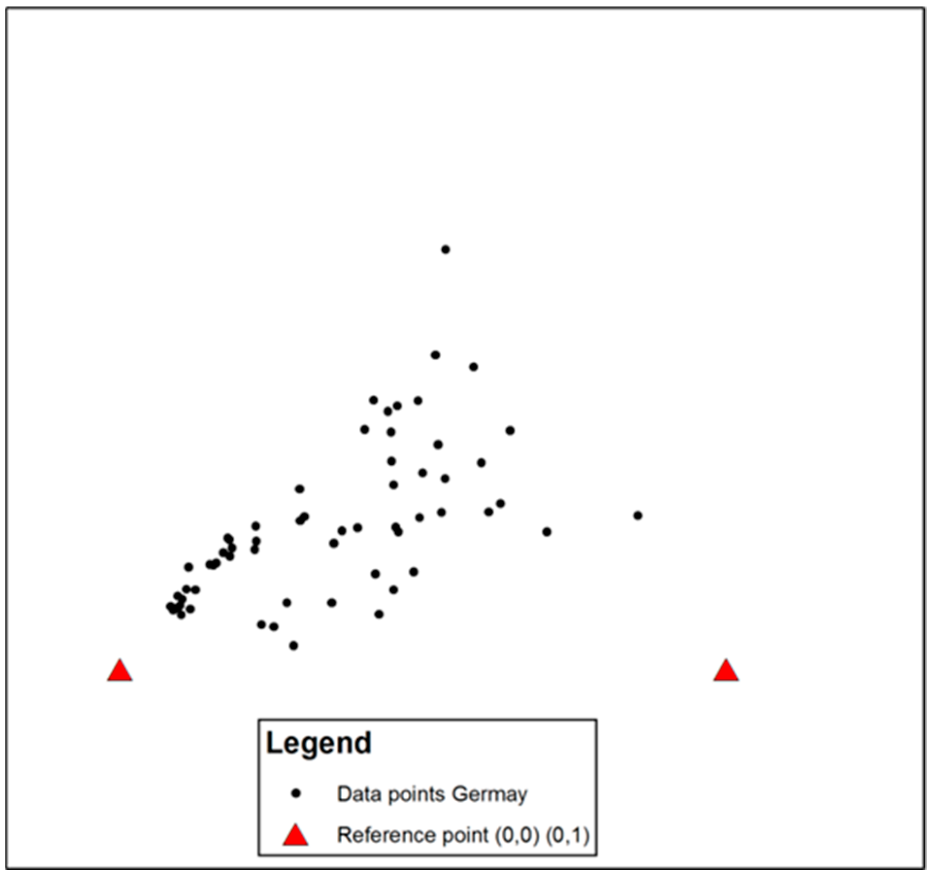
2.4. Data Projection

To visualize the data in an interrelated way with a focus on the USDA soil texture classification, it was integrated into a GIS software. The spatial position of each data point within the USDA textural classification diagram, an equilateral ternary plot, was defined by a triple of data (i.e., % sand/% silt/% clay). To transfer these spatial data into a GIS software, the data triples were transferred into Cartesian coordinates (i.e., 100% sand = (0,0); 100% silt = (0,1); 100% clay = (1/2,√3/2)).
All 61 samples were imported to ArcMap using the X-/Y-values as described above. Two reference points were added to the dataset to visualize 100% sand (0,0) and 100% silt (0,1), and to create a common working base for further interpolations (Figure 1).
To obtain a coherent distribution within the ternary plot, the data was interpolated. To be able to later apply statistical algorithms, the inverse distance weighting (IDW) algorithm was selected to receive an interpolated raster surface. The IDW was used since the data were located relatively close to each other and, furthermore, the IDW is limited to the range of raw data [46]. The searching radius was set to variable and the number of points within the search radius settings was set to 30 for each ternary plot.
Using this procedure, the three measured soil parameters, bulk density, porosity, and thermal conductivity as well as the comparisons between the measured and calculated thermal conductivities, were plotted. Furthermore, various plots with deviations between different thermal conductivities were generated: first, a comparison between the measured thermal conductivities and values calculated after Kersten (1949); second, a comparison between the measured thermal conductivity TK04 results and the values of the lookup table of the ThermoMap project including the three bulk density stages (see Section 3). The classification for the bulk density plot is based on Sponagel (2005) (Table 1).

3. Results

A summary of the measured results is displayed in Table 2. Based on the grain size distribution, nine different grain size classes according to the USDA soil texture classification from various locations (inside Germany) were examined in terms of bulk density, porosity, and thermal conductivity.

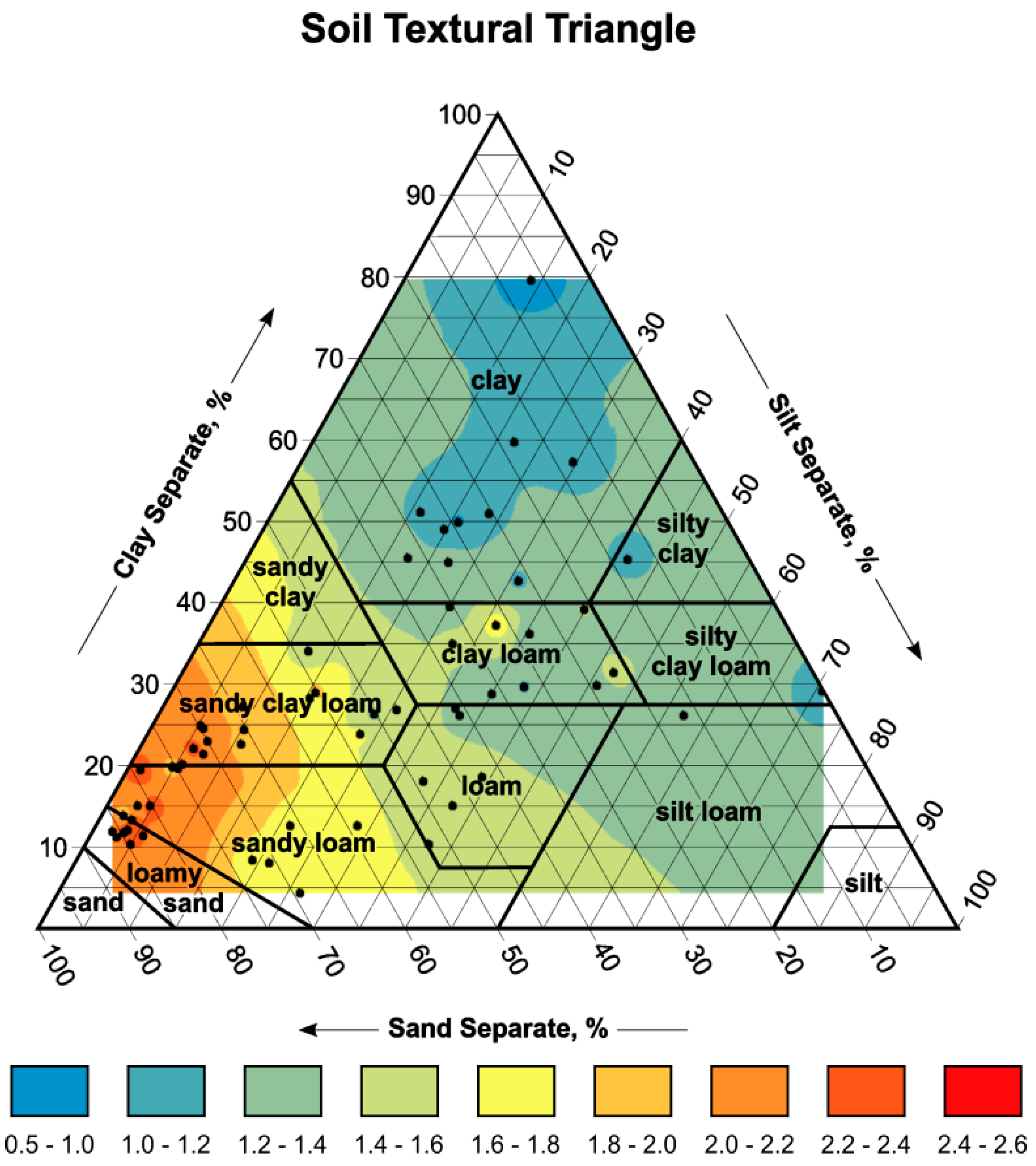
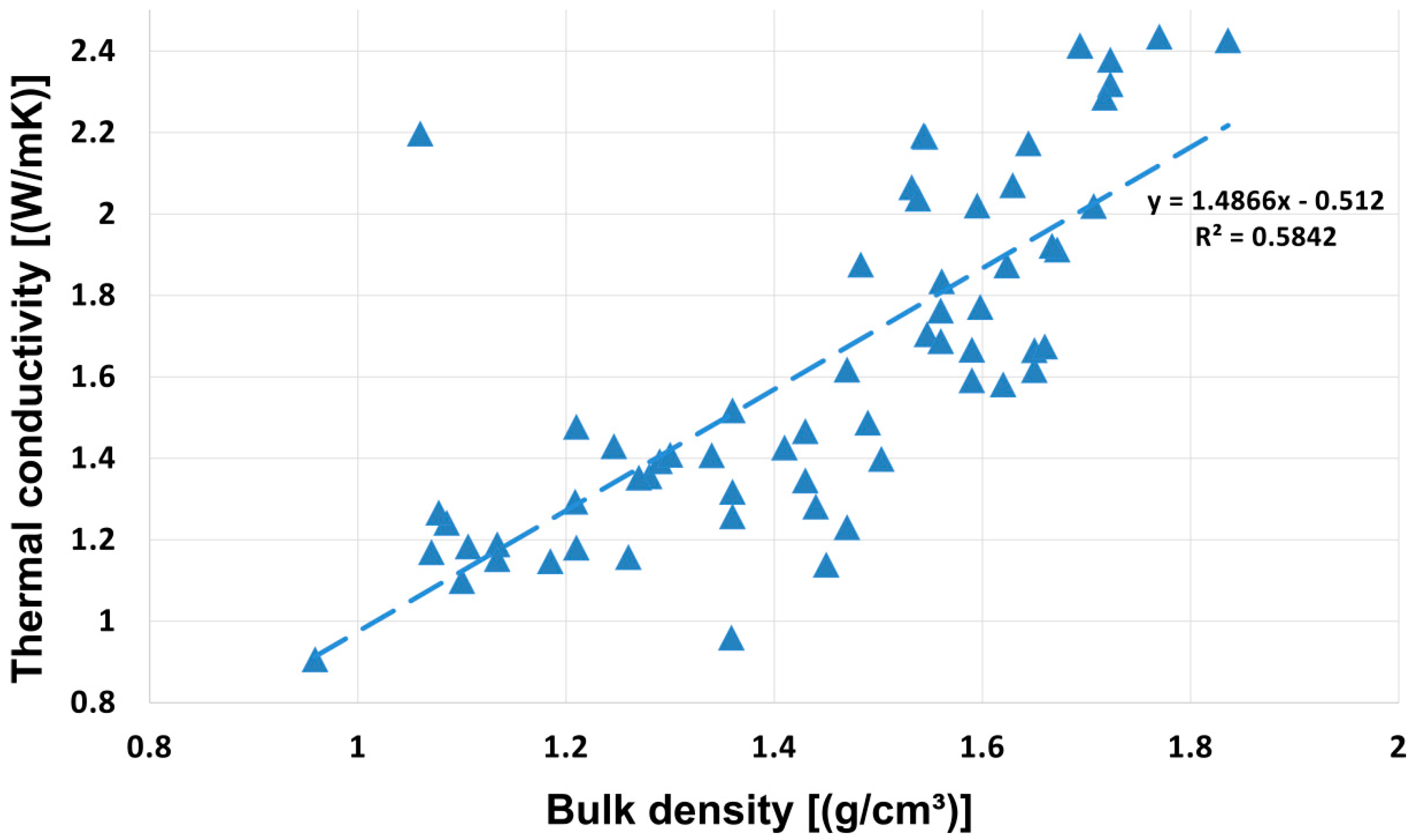
3.1. Bulk Density and Porosity

In general, clayey soils are classified as having low and very low bulk densities (Table 1), ranging from 0.959 g cm³ up to 1.359 g cm³ (Table 2) with an average of 1.127 g cm³. Elevated bulk density values could be observed with an increasing proportion of sand (Figure 2). For sandy clay loam samples, high and marginally very high bulk densities were measured, reaching values of 1.836 g cm³. However, the range of bulk density within each grain size class was quite large, as observable within the loamy sands or clays.
The computed porosities showed an inverse trend when compared to the bulk density (Figure 3), which was not remarkable/surprising since the calculation was based on the measured bulk densities. Porosity decreased with an increasing content of sand. A minimum porosity of 20.5% appeared for loamy sands- and sandy clay loams. Clays, in particular, showed the highest porosities.

3.2. Thermal Conductivity

The two major objectives in this study focused, on the one hand, on the comparison between the measured thermal conductivity values with the TK04 device and the calculated thermal conductivity values when different Kersten formulas were applied (Section 3.2.2). On the other hand, a comparison of the thermal conductivity values with the TK04-measured device and the calculated ThermoMap values for the three different bulk density values (Section 3.2.3) was performed.

3.2.1. Thermal Conductivity Measurements

Figure 4 displays the distribution of thermal conductivity within the USDA soil texture classification. In this case, the coarse material showed higher thermal conductivity values than the fine material.
Regardless of the grain size classes, all measured thermal conductivities were in a range between 0.906 W (m·K)−1 and 2.435 W (m·K)−1 (Table 2). In this range, clay possessed the lowest values, whereas loamy sand and sandy loam showed very high thermal conductivities. However, the spread of the thermal conductivity in the ‘loamy sand’ and ‘sandy loam’ section was relatively high, as they covered a range from 1.581 W (m·K)−1 up to 2.435 W (m·K)−1. This was accompanied by a positive correlation with increasing bulk density (Figure 5).
A positive correlation of thermal conductivity with increasing sand content was observed (Figure 4) as well as a positive correlation between the bulk densities and increasing sand content (Figure 2). Hence, the relation between thermal conductivity and bulk density as displayed in Figure 5 was not surprising.

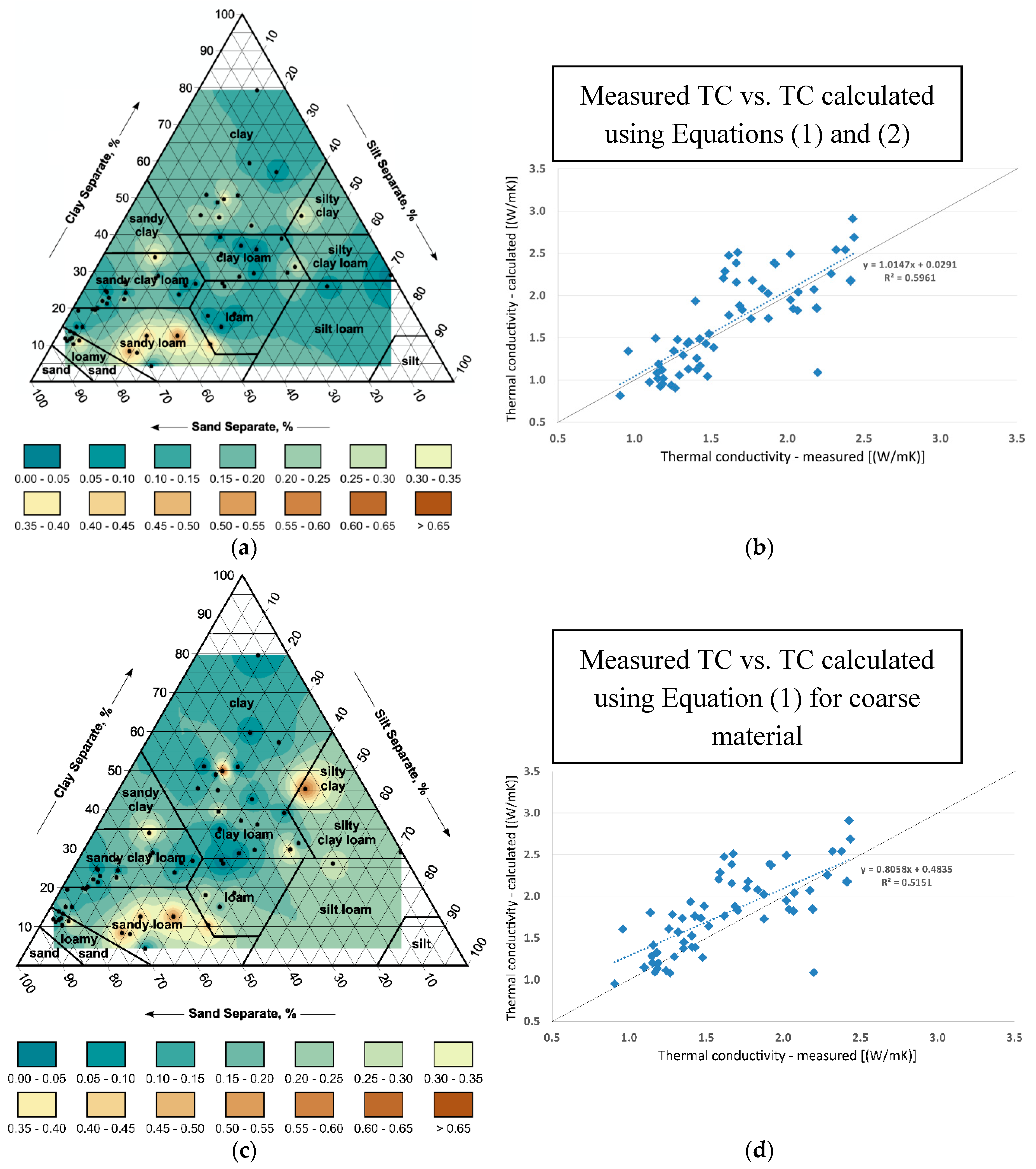
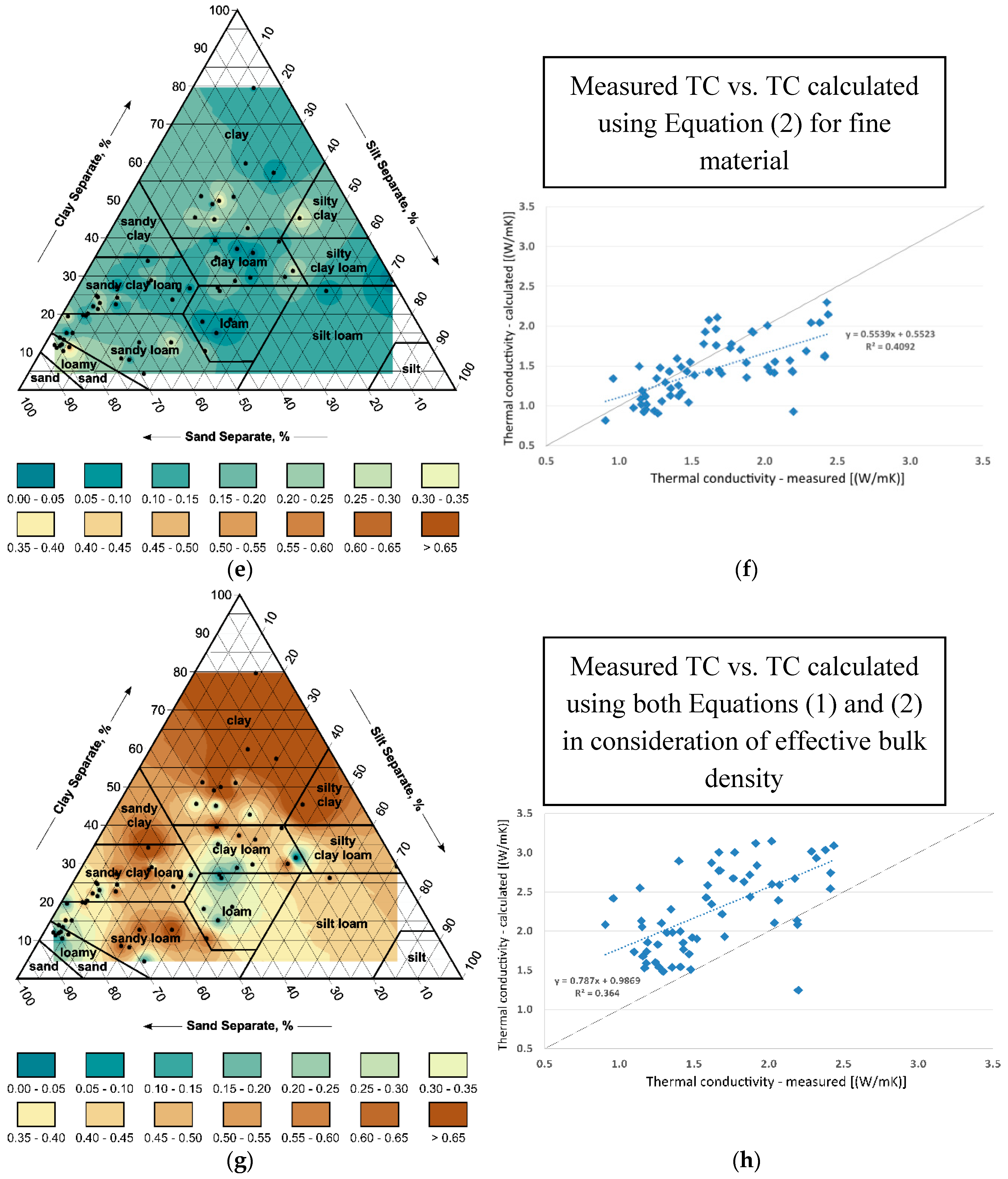
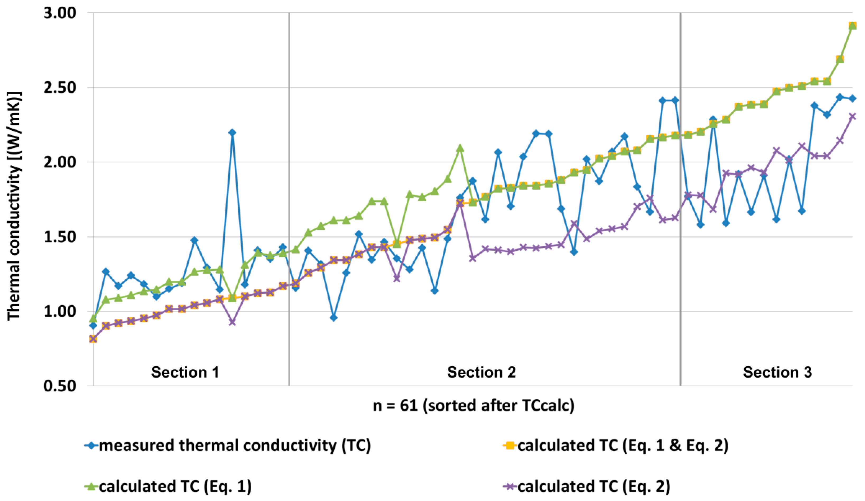
3.2.2. Thermal Conductivity Measurements vs. Kersten Formulas

The best correlation between the measured and calculated thermal conductivity could be achieved by applying the formulas from Kersten (1949), distinguishing between sand- (Equation (1)) and silt-/clay-dominated (Equation (2)) soils as recommended, and using the measured bulk densities for calculation (Figure 6b). When applying only Equation (1) for the sand-dominated soils, the associated regression line showed a pronounced discrepancy from the line through the origin (Figure 6d) at lower thermal conductivities. For high thermal conductivities, the regression line converged to the line through the origin. An inverse trend can be observed in Figure 6f, where the thermal conductivity was calculated by only applying Equation (2). In this case, a better correlation between the measured and calculated thermal conductivities was noticed for soils with low thermal conductivities, and with increasing thermal conductivity, the discrepancy increased.
However, these observations could not be confirmed in Figure 6a,c,e where the mentioned deviations within the thermal conductivities were not visible in relation to the USDA soil texture classification. An overall higher deviation between the measured and calculated thermal conductivities is illustrated by the comparison of Figure 6a,c,e. Deviations between the measured and calculated thermal conductivities, by the recommended application of the Kersten formulas (Figure 6a), showed significant differences, especially for sandy loam (up to 0.55–0.60 W (m·K)−1) but also for sandy clay (≤0.4 W (m·K)−1), and minor differences for sandy clay and loamy sand (≤0.35 W (m·K)−1). Higher contrasts in thermal conductivities, calculated by applying only Equation (1) (Figure 6c), appeared in the areas of sandy loam and silty clay (up to 0.6 W (m·K)−1). The measured thermal conductivities of clay loam, clay as well as sandy clay loam, on the contrary, hardly deviated from the calculated ones. The overall lowest deviations between the calculated and measured thermal conductivities (Figure 6e) occurred by only applying Equation (2). In this case, differences of ≤0.35 W (m·K)−1 appeared within the loamy sand and silty clay.
By calculating the thermal conductivity with the equations according to Kersten (1949) and by using the calculated effective bulk density (Equation (4)) instead of the measured one, a distinct larger gap in relation to the measured thermal conductivity was observable (Figure 6h). The calculated thermal conductivities were accounted/lifted roughly 1.0 W (m·K)−1 above the measured thermal conductivities. This relationship is also reflected in Figure 6g where a strong deviation between the measured and calculated thermal conductivities was implied. This observation was true for nearly all of the data points and classes, except for some areas within clay loam, loam, and loamy sand.
The calculated thermal conductivities for soils in the uppermost depths stage of 0–3 m and a standardized bulk density of 1.3 g cm³ ranged from ~1.2 W (m·K)−1 to ~1.5 W (m·K)−1 (Figure 7). The regression line (Figure 7) had a much lower slope of 0.2107 than the line through the origin.

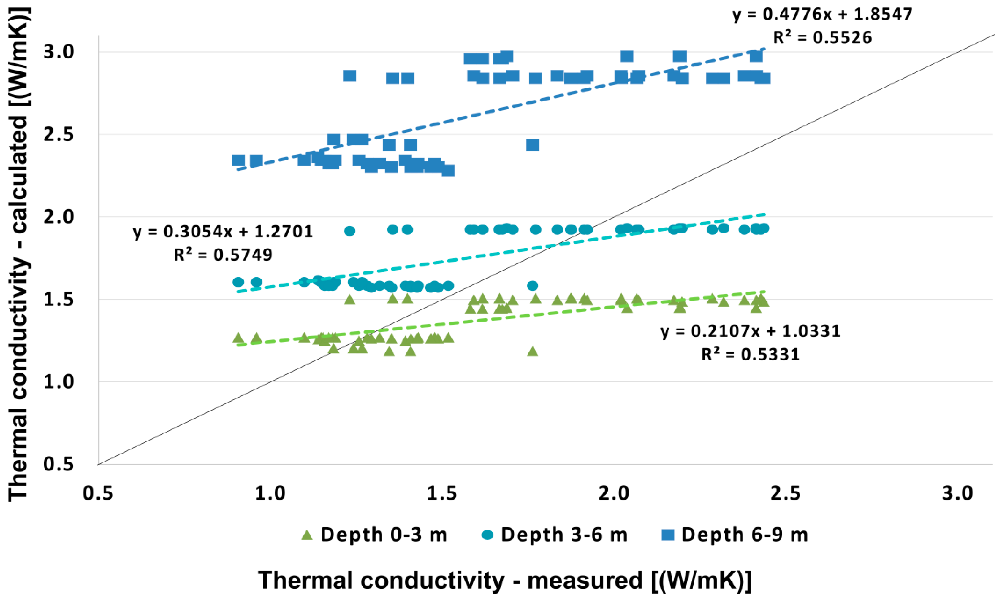
3.2.3. Thermal Conductivity Measurements vs. ThermoMap Values

This slight underestimation is also reflected in Figure 8, where positive and negative deviation of the ThermoMap project values from the thermal conductivities measured with the TK04 were related to the USDA soil texture classification. In particular, sand rich areas (loamy sand, sandy loam, and sandy clay loam) strongly deviated negatively (down to 0.42 W (m·K)−1) from the measured values. In contrast, clays were rather overestimated with a difference in thermal conductivity of up to 0.30 W (m·K)−1. By using a standardized bulk density of 1.5 g cm³, representing soils at depths of 3–6 m, for calculating thermal conductivity after Kersten (1949), a better fit was achieved. The values generally deviated less from the best fit when compared to the ones calculated for a depth range of 0–3 m. However, a general overestimation of the calculated thermal conductivities calculated with a standardized bulk density of 1.5 g cm³ was observed in Figure 9. A maximum positive deviation of 0.55 W (m·K)−1 was reached for clay, whereas loamy sand, sandy loam, and sandy clay loam were still underestimated (down to −0.27 W (m·K)−1). The thermal conductivities calculated for soils at a depth of 6–9 m, with an expected bulk density of 1.8 g cm³, generally showed an unfavorable correlation with the measured thermal conductivity values (Figure 7). This was reflected in the calculated thermal conductivities deviating at least ~0.4 W (m·K)−1 from the highest and ~1.3 W (m·K)−1 from the lowest measured thermal conductivities.
The databases for Figure 8, Figure 9 and Figure 10 are listed in an overview table (Table 3) where the thermal conductivity values for all respective bulk densities, which were defined in the ThermoMap project, were collated.
This observation was confirmed in the soil textural triangle (Figure 10), accounting for a strong positive deviation of up to 1.10 W (m·K)−1 (for clays) calculated from the measured thermal conductivities. The smallest deviations in thermal conductivities were determined for loamy sands, silt-poor sandy loams, and silt-poor sandy clay loams.
When comparing the measured thermal conductivities with the values calculated and sorted after Kersten (1949) (Figure 11), thereby distinguishing between the conventional method using both Equations (1) and (2), and just using either one of the formulas, several observations were apparent. With the exception of two samples, the equation used for the samples with a sand proportion below 50% was applied to all soils with a calculated low thermal conductivity. Whereas for all soils with a calculated high thermal conductivity, the equation for sand proportions above 50% was used. Furthermore, the thermal conductivities calculated solely with Equation (2) always possessed lower values than when calculated with Equation (1). In the area of the lowest thermal conductivities (Section 1/Figure 11), the measured values correlated with the predicted ones that used the Equation (1), although these samples comprised only clayey/silty soils.
Decent accordance was achieved in the middle section between the measured and thermal conductivities predicted with the conventional method. Section 3 shows the measured thermal conductivities that were in agreement with values predicted with Equation (2), despite the samples being sandy soils.

4. Discussion

The aim of this study was to compare the thermal conductivity values derived by the laboratory TK04 measurements and hypothetical soil properties derived from the ThermoMap project and their visualization in USDA textural classes. Bulk densities should preferably be used for thermal conductivity calculations according to Kersten (1949). Generally, for calculating thermal conductivity, a bulk density of about 1.5 g cm−3 fits best. However, an even better result was achieved by distinguishing between certain grain size classes and applied bulk densities. Clay soils were represented best by using the bulk density of 1.3 g cm−3 (Figure 8), whereas a bulk density of 1.8 g cm³ only provided suitable outcomes for very pure sands (Figure 10). All of the other intermediate grain size classes such as loamy sand, sandy loam, or silts should be calculated with an assumed bulk density of 1.5 g cm−3 (Figure 9). These results corresponded to the bulk density ranges stated by Chaudhari et al. (2013), although a high clay content could mask the effect of an increased organic content [1,2]. In contrast to coarse soils [47], clays possess a relatively high porosity, resulting in lower bulk densities.
Computing thermal conductivity with effective bulk density provided unrealistic high values (Figure 6g and Table 2). This was also observed by Renger et al. (2008), who proposed that the calculation factor for computing the effective bulk density of 0.0009 applied in Equation (4) was too high. This may be due to the predominantly medium to high organic content of the soils, where the factor was derived from [48]. Operating with effective bulk densities showed the highest deviations in fine grained soils (Figure 6g), despite having been particularly developed for this fine grain size fraction.
It must be considered that although a consistent pressure load was applied by measuring with the TK04, different bulk densities were generated dependent on the respective compactibility of each grain size class (Figure 3). Still, the relation between bulk density and thermal conductivity showed a low coefficient of correlation (Figure 5). Thus, bulk density does not solely control the thermal conductivity of soils. Other crucial factors are the degree of saturation (θ), volume fraction of air (n) as well as the volume fraction of solids (νs) [21,28,30,49]. Additionally, mineral type and grain size distribution are decisive for the thermal conductivity of soils [50]. As all samples in this study were measured under saturated conditions, the degree of saturation and volume fraction of air could be neglected. Moreover, a mineralogical test was not conducted. Consequently, only grain size distribution was taken into account.
Clays and silts, in contrast to sandy soils, have a very high porosity (Figure 4), which results in lower bulk densities [47]. As a consequence, by measuring under saturated conditions, the relative amount of water in clays/silts was much higher than in sandy soils. Water intrinsically has a much lower thermal conductivity of ~0.6 W (m·K)−1 [51] than most minerals with values >1.9 W (m·K)−1. Furthermore, the amount of quartz minerals that possess very high thermal properties of up to 7.7 W (m·K)−1 [52,53] was lower in clayey/silty than in sandy soils. Altogether, this led to the decreased thermal conductivities of fine grained soils in contrast to sandy soils. The observations made within this study were thereby in agreement with the results of Brigaud and Vasseur (1989) [52]. Referring to the factors investigated in this study such as bulk density, grain size, and mineralogy, Zhang et al. (2017) reported similar results [50]. This regarded the positive correlation between increasing bulk density, particle size, and thermal conductivity.
When the critical moisture content is reached, thermal conductivity does not further increase significantly. According to Zhang et al. (2017), the critical moisture content of clay-/silt-soils is much higher when compared to that of sandy soils. As a consequence, the calculated thermal conductivities representing high water contents or completely saturated soils are likely to be overestimated, especially for sands (Figure 11).
The reason for the larger fluctuations within the sandy soils when compared to the clayey/silty soils was not thoroughly investigated in this study. However, these fluctuations might be caused by mineralogical variations, different bulk densities, or device-related measurement errors. Furthermore, dynamic hydraulic processes were not considered. However, to measure comparable thermal conductivities, a constant water content is crucial.
In times of fossil fuel shortage [54], all research in the fields of renewable energy systems is fundamental to develop alternative energy concepts for heating and cooling, for example, by the usage of geothermal heat pumps that will increase massively over the next few decades [55]. Detailed knowledge about thermo-physical soil properties is notably beneficial when planning very shallow geothermal systems due to their impact on the efficiency of geothermal installations. Research on thermal conductivity, such as this study, is the foundation for a proper soil assessment regarding sustainable energy supply.

5. Conclusions

Under saturated conditions, the higher the amount of sand or quartz grains, respectively, the higher the thermal conductivity of soil. Additionally, a high bulk density significantly improves thermal conductivity. From the comparison of various thermal conductivities with the measured and classified values as well as different calculations using the formulas after Kersten, the following conclusions can be drawn. Regular bulk density provided the best fit with the formulas to calculate thermal conductivity, whereas effective bulk density led to an overestimation. Furthermore, to calculate thermal conductivity, both Kersten-formulas should be used accordingly and not just one of them.
Due to the comparison between the calculated values according to Bertermann et al. (2014) and the measured TK04 thermal conductivity measurements, an approximation between the laboratory TK04 measurements and actual thermal soil properties could be made. The thermal conductivity values measured with the TK04 can be associated with a depth of 3–6 m based on the ThermoMap depth classification [7], which is in the depth range of very shallow geothermal systems like heat baskets. The collector systems are usually installed at a depth of 1.5 m, which corresponded to lower thermal conductivity values than those measured with the TK04 device. With the evaluated and soil-type-depending thermal conductivities, the system of shallow geothermal heat exchange can be understood more precisely. It should be noted that the measured thermal conductivity values for each grain size class in the mentioned depth represented conditions below the water surface as the TK04 measurements were performed under saturated conditions.

Author Contributions

Conceptualization, D.B.; Methodology, D.B., H.S., J.M., and S.F.; Software, J.M.; Validation, S.F. and J.M.; Formal Analysis, H.S.; Investigation, S.F.; Resources, D.B.; Writing—Original Draft Preparation, H.S. and S.F.; Writing—Review & Editing, D.B. and J.M.; Visualization, J.M.; Supervision, D.B.; Project Administration, D.B.; Funding Acquisition, D.B.

Funding

This work was co-funded by the European Commission: “ThermoMap” project (grant number 250446).

Acknowledgments

We want to thank our master’s students Christopher Weindl and Sebastian Claus for all their effort during the laboratory analysis and test field investigations. Further thanks to Viktor Iancu for cross-reading and discussions.

Conflicts of Interest

The authors declare no conflict of interest.

Nomenclature

λ [W (m·K)−1]thermal conductivity (TC)
ϕ [-]porosity
ρb [g cm³]bulk density (BD)
ρs [g cm³]density, soil components
θW [-]water content (WC)
Sp [-]amount of saturated pore volume
md [g]mass, dry
θ [-]degree of saturation
Vc [cm3]Volume, cylinder
n [cm3]volume, fraction of air
ρb, eff [g cm−3]bulk density, effective
vs [cm3]volume, fraction of solids
nc [-]amount of clay content

References

  1. Bayer, P.; Saner, D.; Bolay, S.; Rybach, L.; Blum, P. Greenhouse gas emission savings of ground source heat pump systems in Europe: A review. Renew. Sustain. Energy Rev. 2012, 16, 1256–1267. [Google Scholar] [CrossRef]
  2. Blum, P.; Campillo, G.; Münch, W.; Kölbel, T. CO2 savings of ground source heat pump systems—A regional analysis. Renew. Energy 2010, 35, 122–127. [Google Scholar] [CrossRef]
  3. Dickinson, J.; Jackson, T.; Matthews, M.; Cripps, A. The economic and environmental optimisation of integrating ground source energy systems into buildings. Energy 2009, 34, 2215–2222. [Google Scholar] [CrossRef]
  4. Bense, V.F.; Kooi, H. Temporal and spatial variations of shallow subsurface temperature as a record of lateral variations in groundwater flow: Geothermal Data around Shallow Fault Zone. J. Geophys. Res. Solid Earth 2004, 109. [Google Scholar] [CrossRef]
  5. Hähnlein, S.; Bayer, P.; Ferguson, G.; Blum, P. Sustainability and policy for the thermal use of shallow geothermal energy. Energy Policy 2013, 59, 914–925. [Google Scholar] [CrossRef]
  6. Bertermann, D.; Bialas, C.; Morper-Busch, L.; Klug, H.; Rohn, J.; Stollhofen, M.P.; Jaudin, F.; Maragna, C.M.; Einarsson, G.M.; Vikingsson, S. ThermoMap—An open-source web mapping application for illustrating the very shallow geothermal potential in Europe and selected case study areas. In Proceedings of the European Geothermal Congress 2013, Pisa, Italy, 3–7 June 2013; pp. 1–7. [Google Scholar]
  7. Bertermann, D.; Klug, H.; Morper-Busch, L.; Bialas, C. Modelling vSGPs (very shallow geothermal potentials) in selected CSAs (case study areas). Energy 2014, 71, 226–244. [Google Scholar] [CrossRef]
  8. Bertermann, D.; Klug, H.; Morper-Busch, L. A pan-European planning basis for estimating the very shallow geothermal energy potentials. Renew. Energy 2015, 75, 335–347. [Google Scholar] [CrossRef]
  9. Dehner, U. Bestimmung der thermischen Eigenschaften von Böden als Grundlage für die Erdwärmenutzung. Mainz. Geowiss. Mitteilungen 2007, 35, 159–186. [Google Scholar]
  10. Hähnlein, S.; Bayer, P.; Blum, P. International legal status of the use of shallow geothermal energy. Renew. Sustain. Energy Rev. 2010, 14, 2611–2625. [Google Scholar] [CrossRef]
  11. Salata, F.; Nardecchia, F.; Gugliermetti, F.; de Lieto Vollaro, A. How thermal conductivity of excavation materials affects the behavior of underground power cables. Appl. Therm. Eng. 2016, 100, 528–537. [Google Scholar] [CrossRef]
  12. De Lieto Vollaro, R.; Fontana, L.; Vallati, A. Experimental study of thermal field deriving from an underground electrical power cable buried in non-homogeneous soils. Appl. Therm. Eng. 2014, 62, 390–397. [Google Scholar] [CrossRef]
  13. De Lieto Vollaro, R.; Fontana, L.; Vallati, A. Thermal analysis of underground electrical power cables buried in non-homogeneous soils. Appl. Therm. Eng. 2011, 31, 772–778. [Google Scholar] [CrossRef]
  14. Ocłoń, P.; Cisek, P.; Rerak, M.; Taler, D.; Rao, R.V.; Vallati, A.; Pilarczyk, M. Thermal performance optimization of the underground power cable system by using a modified Jaya algorithm. Int. J. Therm. Sci. 2018, 123, 162–180. [Google Scholar] [CrossRef]
  15. Janda, K.; Málek, J.; Recka, L. Influence of renewable energy sources on transmission networks in Central Europe. Energy Policy 2017, 108, 524–537. [Google Scholar] [CrossRef]
  16. Komendantova, N.; Battaglini, A. Social Challenges of Electricity Transmission: Grid Deployment in Germany, the United Kingdom, and Belgium. IEEE Power Energy Mag. 2016, 14, 79–87. [Google Scholar] [CrossRef] [Green Version]
  17. Gouda, O.E.S.; Osman, G.F.; Salem, W.; Arafa, S. Cyclic Loading of Underground Cables Including the Variations of Backfill Soil Thermal Resistivity and Specific Heat with Temperature Variation. IEEE Trans. Power Deliv. 2018. [Google Scholar] [CrossRef]
  18. Ocłoń, P.; Bittelli, M.; Cisek, P.; Kroener, E.; Pilarczyk, M.; Taler, D.; Rao, R.V.; Vallati, A. The performance analysis of a new thermal backfill material for underground power cable system. Appl. Therm. Eng. 2016, 108, 233–250. [Google Scholar] [CrossRef]
  19. Côté, J.; Konrad, J.-M. Thermal conductivity of base-course materials. Can. Geotech. J. 2005, 42, 61–78. [Google Scholar] [CrossRef]
  20. Logsdon, S.D.; Green, T.R.; Bonta, J.V.; Seyfried, M.S.; Evett, S.R. Comparison of Electrical and Thermal Conductivities for Soils From Five States. Soil Sci. 2010, 175, 573–578. [Google Scholar] [CrossRef]
  21. Ochsner, T.E.; Horton, R.; Ren, T. A new perspective on soil thermal properties. Soil Sci. Soc. Am. J. 2001, 65, 1641–1647. [Google Scholar] [CrossRef]
  22. Clauser, C. Einführung in Die Geophysik: Globale Physikalische Felder und Prozesse in der Erde; Lehrbuch; Springer Spektrum: Berlin/Heidelberg, Germany, 2014; ISBN 978-3-642-04495-3. [Google Scholar]
  23. Horai, K.; Simmons, G. Thermal conductivity of rock-forming minerals. Earth Planet. Sci. Lett. 1969, 6, 359–368. [Google Scholar] [CrossRef]
  24. Kersten, M.S. Thermal Properties of Soils. Available online: https://conservancy.umn.edu/handle/11299/124271 (accessed on 24 July 2018).
  25. Chaudhari, P.R.; Ahire, D.V.; Ahire, V.D.; Chkravarty, M.; Maity, S. Soil bulk density as related to soil texture, organic matter content and available total nutrients of Coimbatore soil. Int. J. Sci. Res. Publ. 2013, 3, 1–8. [Google Scholar]
  26. Saxton, K.E.; Rawls, W.J. Soil Water Characteristic Estimates by Texture and Organic Matter for Hydrologic Solutions. Soil Sci. Soc. Am. J. 2006, 70, 1569–1578. [Google Scholar] [CrossRef]
  27. Abu-Hamdeh, N.H. Thermal Properties of Soils as affected by Density and Water Content. Biosyst. Eng. 2003, 86, 97–102. [Google Scholar] [CrossRef]
  28. Abu-Hamdeh, N.H.; Reeder, R.C. Soil Thermal Conductivity Effects of Density, Moisture, Salt Concentration, and Organic Matter. Soil Sci. Soc. Am. J. 2000, 64, 1285–1290. [Google Scholar] [CrossRef]
  29. Bertermann, D.; Schwarz, H. Laboratory device to analyse the impact of soil properties on electrical and thermal conductivity. Int. Agrophys. 2017, 31, 157–166. [Google Scholar] [CrossRef] [Green Version]
  30. Farouki, O.T. Thermal Properties of Soils; Cold Regions Research and Engineering Laboratory: Hanover, NH, USA, 1981; p. 151. [Google Scholar]
  31. Lu, S.; Ren, T.; Gong, Y.; Horton, R. An Improved Model for Predicting Soil Thermal Conductivity from Water Content at Room Temperature. Soil Sci. Soc. Am. J. 2007, 71, 8–14. [Google Scholar] [CrossRef]
  32. Chen, S.X. Thermal conductivity of sands. Heat Mass Transf. 2008, 44, 1241–1246. [Google Scholar] [CrossRef]
  33. Haigh, S.K. Thermal conductivity of sands. Géotechnique 2012, 62, 617–625. [Google Scholar] [CrossRef]
  34. Lu, Y.; Lu, S.; Horton, R.; Ren, T. An Empirical Model for Estimating Soil Thermal Conductivity from Texture, Water Content, and Bulk Density. Soil Sci. Soc. Am. J. 2014, 78, 1859–1868. [Google Scholar] [CrossRef]
  35. Markert, A.; Bohne, K.; Facklam, M.; Wessolek, G. Pedotransfer Functions of Soil Thermal Conductivity for the Textural Classes Sand, Silt, and Loam. Soil Sci. Soc. Am. J. 2017, 81, 1315–1327. [Google Scholar] [CrossRef]
  36. Decagon Devices, Inc. KD2 Pro Thermal Properties Analyzer—Operator’s Manual; Decagon Devices, Inc.: Pullmann, WA, USA, 2016; p. 71. [Google Scholar]
  37. Seibertz, K.S.O.; Chirila, M.A.; Bumberger, J.; Dietrich, P.; Vienken, T. Development of in-aquifer heat testing for high resolution subsurface thermal-storage capability characterisation. J. Hydrol. 2016, 534, 113–123. [Google Scholar] [CrossRef]
  38. United States Department of Agriculture. USDA Textural Soil Classification; Soil Mechanics Level 1; USDA: Washington, DC, USA, 1987. [Google Scholar]
  39. Johansen, O. Thermal Conductivity of Soils; Corps of Engineers, U.S. Army, Cold Regions Research and Engineering Laboratory: Hanover, NH, USA, 1977. [Google Scholar]
  40. Wessolek, G.; Stoffregen, H.; Täumer, K. Persistency of flow patterns in a water repellent sandy soil—Conclusions of TDR readings and a time-delayed double tracer experiment. J. Hydrol. 2009, 375, 524–535. [Google Scholar] [CrossRef]
  41. Xiao, B.; Zhang, X.; Wang, W.; Long, G.; Chen, H.; Kang, H.; Ren, W. A Fractal Model for Water Flow through Unsaturated Porous Rocks. Fractals 2018, 26, 1840015. [Google Scholar] [CrossRef]
  42. Bodenkundliche Kartieranleitung: Mit 103 Tabellen und 31 Listen, 5th ed.; Sponagel, H. (Ed.) Verbesserte und Erweiterte Auflage; E. Schweizerbart’sche Verlagsbuchhandlung (Nägele und Obermiller): Stuttgart, Germany, 2005; ISBN 978-3-510-95920-4. [Google Scholar]
  43. Andersland, O.B.; Anderson, D.M. (Eds.) Geotechnical Engineering for Cold Regions; McGraw-Hill: New York, NY, USA, 1978; ISBN 0-07-001615-1. [Google Scholar]
  44. Blackwell, J.H. A Transient-Flow Method for Determination of Thermal Constants of Insulating Materials in Bulk Part I—Theory. J. Appl. Phys. 1954, 25, 137–144. [Google Scholar] [CrossRef]
  45. Davis, M.G.; Chapman, D.S.; Van Wagoner, T.M.; Armstrong, P.A. Thermal conductivity anisotropy of metasedimentary and igneous rocks. J. Geophys. Res. 2007, 112. [Google Scholar] [CrossRef] [Green Version]
  46. Watson, D.F.; Philip, G.M. A refinement of inverse distance weighted interpolation. Geo-Processing 1985, 2, 315–327. [Google Scholar]
  47. Park, J.; Santamarina, J.C. Revised Soil Classification System for Coarse-Fine Mixtures. J. Geotech. Geoenviron. Eng. 2017, 143, 04017039. [Google Scholar] [CrossRef]
  48. Renger, M.; Bohne, K.; Facklam, M.; Harrach, T.; Riek, W.; Schäfer, W.; Wessolek, G.; Zacharias, S. Ergebnisse und Vorschläge der DBG-Arbeitsgruppe „Kennwerte des Bodengefüges “zur Schätzung bodenphysikalischer Kennwerte; DBG-Arbeitsgruppe: Berlin, Germany, 2008. [Google Scholar]
  49. Alrtimi, A.; Rouainia, M.; Haigh, S. Thermal conductivity of a sandy soil. Appl. Therm. Eng. 2016, 106, 551–560. [Google Scholar] [CrossRef]
  50. Zhang, T.; Cai, G.; Liu, S.; Puppala, A.J. Investigation on thermal characteristics and prediction models of soils. Int. J. Heat Mass Transf. 2017, 106, 1074–1086. [Google Scholar] [CrossRef]
  51. Cosenza, P.; Guérin, R.; Tabbagh, A. Relationship between thermal conductivity and water content of soils using numerical modelling. Eur. J. Soil Sci. 2003, 54, 581–588. [Google Scholar] [CrossRef]
  52. Brigaud, F.; Vasseur, G. Mineralogy, porosity and fluid control on thermal conductivity of sedimentary rocks. Geophys. J. Int. 1989, 98, 525–542. [Google Scholar] [CrossRef] [Green Version]
  53. Tarnawski, V.-R.; Leong, W.H. Thermal Conductivity of Soils at Very Low Moisture Content and Moderate Temperatures. Transp. Porous Media 2000, 41, 137–147. [Google Scholar] [CrossRef]
  54. Ediger, V.Ş.; Hoşgör, E.; Sürmeli, A.N.; Tatlıdil, H. Fossil fuel sustainability index: An application of resource management. Energy Policy 2007, 35, 2969–2977. [Google Scholar] [CrossRef]
  55. Fridleifsson, I.; Bertani, R.; Huenges, E.; Lund, J.W.; Rybach, L. The Possible Role and Contribution of Geothermal Energy to the Mitigation of Climate Change; Intergovernmental Panel on Climate Change (IPCC): Geneva, Switzerland, 2008; pp. 59–80. [Google Scholar]
Figure 1. Visualization of the shapefile used for further interpolations.
Soilsystems 02 00050 g001
Figure 2. Bulk density [g cm³] distribution dependent on the textural soil classification.
Soilsystems 02 00050 g002
Figure 3. Distribution of porosity [-] dependent on the USDA textural soil classification.
Soilsystems 02 00050 g003
Figure 4. Distribution of measured thermal conductivity [W (m·K)−1] for the different textural soil classes.
Soilsystems 02 00050 g004
Figure 5. Bulk density plotted against the thermal conductivities measured with the TK04.
Soilsystems 02 00050 g005
Figure 6. (a) Deviation (%) of the thermal conductivity values using the Kersten formulas (Equations (1) and (2)) from the TK04 measurements; (b) Plot of the measured versus the calculated thermal conductivities after Kersten (Equations (1) and (2)) (Linear regression line = black dashed line); (c) Deviation (%) of the thermal conductivity values using the Kersten formula (Equation (1)) from the TK04 measurement; (d) Plot of the measured versus the calculated thermal conductivities after Kersten (Equation (1)) (Linear regression line = black dashed line); (e) Deviation (%) of the thermal conductivity values using the Kersten formula (Equation (2)) from the TK04 measurements; (f) Plot of the measured versus the calculated thermal conductivities after Kersten (Equation (2)) (Linear regression line = black dashed line); (g) Deviation (%) of the thermal conductivity values using the Kersten formulas (Equations (1) and (2)) and effective bulk density values from the TK04 measurements; (h) Plot of the measured versus the calculated thermal conductivities after Kersten using the effective bulk densities instead of standard bulk densities. (Linear regression line = black dashed line).
Soilsystems 02 00050 g006aSoilsystems 02 00050 g006b
Figure 7. The measured vs. calculated thermal conductivities according to Kersten (1949) for varying soil depths; i.e., bulk densities according to the ThermoMap project.
Soilsystems 02 00050 g007
Figure 8. Positive and negative deviation of the ThermoMap values (BD = 1.3 g cm−3) from the TK04 measured thermal conductivities.
Soilsystems 02 00050 g008
Figure 9. Positive and negative deviation of the ThermoMap values (BD = 1.5 g cm−3) from the TK04 measured thermal conductivities.
Soilsystems 02 00050 g009
Figure 10. Positive deviation of the ThermoMap values (BD = 1.8 g cm−3) from the TK04 measured thermal conductivities.
Soilsystems 02 00050 g010
Figure 11. Comparison between the measured (TK04 results) and calculated thermal conductivities. The calculations according to both Kersten (1949) equations are displayed (sand formula, Equation (1); clay formula, Equation (2)). The values were sorted after the calculated thermal conductivity corresponded to both soil dependent formulas (Equation (1) > 50% sand; Equation (2) < 50% sand).
Soilsystems 02 00050 g011
Table 1. Classification of bulk density ranges according to [42].
ClassificationBulk Density [g/cm3]
very low<1.2
low1.2–1.4
medium1.4–1.6
high1.6–1.8
very high>1.8
Table 2. Data table with the results of all samples investigated. Bulk density and one thermal conductivity (TK04-column) were measured by the TK04 device. Porosity and thermal conductivity according to Kersten (1949) were both computed based on the outcomes of the performed measurements of this study. The third calculated thermal conductivity was provided by the ThermoMap project. Textural soil classes were derived based on the samples granulometry.
Sample-IDTextural Soil ClassBulk Density [g/cm³]Porosity [%]Thermal Conductivity [W (m·K)−1]
TK04Kersten (1949)
I3Loamy Sand1.06060.02.1971.088
II2bSandy Loam1.56141.01.8342.080
II3aLoamy Sand1.72335.02.3182.542
III2aSandy Clay Loam1.59840.01.7712.179
III2bSandy Clay Loam1.83631.02.4262.910
III3aSandy Clay Loam1.50343.01.3981.934
III3bClay Loam1.24653.01.4291.169
III4bSandy Clay Loam1.67237.01.9122.388
III5aClay1.35949.00.9591.341
III5bSandy Loam1.70736.02.0192.493
IV2bClay0.95964.00.9060.815
IV3aClay1.18555.01.1471.084
IV3bClay1.13457.01.1881.017
IV4Clay1.13457.01.1521.017
RD2Clay1.08554.61.2410.936
RD3Clay1.10652.61.1830.954
RD4Clay1.07850.41.2660.904
RD5Sandy Loam1.54724.61.7041.831
RD6Clay Loam1.07156.21.1690.924
RD7Loam1.20945.21.2931.057
RE1Sandy Clay Loam1.59523.92.0201.949
RE2Sandy Clay Loam1.53226.62.0651.823
RE3Sandy Clay Loam1.71821.02.2852.258
RE4Sandy Loam1.64422.92.1732.072
RE5Sandy Clay Loam1.62423.61.8732.025
RE6Sandy Loam1.62923.62.0702.041
RF1Sandy Clay Loam1.48328.91.8751.730
RF2Loamy Sand1.69420.52.4122.170
RF3Loamy Sand1.56025.51.6871.880
RF4Sandy Loam1.69421.02.4132.182
RF5Loamy Sand1.54526.52.1891.856
RF6Loamy Sand1.53826.92.0371.844
RF7Loamy Sand1.54426.12.1921.845
RI-2Silt Loam1.26052.41.1571.189
RI-5Sandy Clay Loam1.59039.91.6662.156
RIII-2Silty Clay1.45045.11.1381.494
RIII-5Clay Loam1.36043.01.3171.294
RIV-1bSandy Clay Loam1.28051.61.3551.452
RIV-2Clay Loam1.21054.51.1801.119
RIV-4Clay Loam1.44045.61.2811.478
RIX-1Clay1.10058.41.0980.974
RVIII-2Loamy Sand1.77033.12.4352.688
V2Sandy Loam1.66737.01.9212.373
VA2Clay Loam1.34043.01.4071.257
VA3Clay Loam1.56043.01.7621.725
VA4Clay Loam1.43043.01.3451.431
VA5Loam1.49042.01.4871.548
VA6Sandy Loam1.65052.01.6162.475
VA7Sandy Loam1.65043.01.6652.385
VA8Sandy Loam1.66052.01.6742.510
VA9Sandy Loam1.62036.01.5812.205
VB1Sandy Clay Loam1.47035.01.2301.767
VB10Sandy Loam1.59054.01.5912.286
VB2Clay Loam1.21043.01.4771.043
VB3Sandy Clay Loam1.36054.01.5171.384
VB5Loam1.30036.01.4081.122
VB6Loam1.27042.01.3521.129
VB7Silty Clay Loam1.36048.81.2571.344
VB8Loam1.43043.01.4661.431
VB9Loam1.41054.01.4261.488
VI3bSandy Loam1.72335.02.3782.542
Table 3. TK04-measured thermal conductivities (TC) for each classified soil sample and three calculated ThermoMap thermal conductivity values; each column has one single bulk density (BD) value. The three different bulk density values represent the depth layers 0–3 m, 3–6 m, and 6–10 m [7].
Sample-IDTextural Soil ClassTC (TK04) [W/(m·K)]TC ThermoMap [W (m·K)−1] (BD = 1.3 g cm³)TC ThermoMap [W (m·K)−1] (BD = 1.5 g cm³)TC ThermoMap [W (m·K)−1] (BD = 1.8 g cm³)
I3Loamy Sand2.1971.411.782.50
II2bSandy Loam1.8341.421.772.51
II3aLoamy Sand2.3181.411.782.50
III2aSandy Clay Loam1.7711.431.772.50
III2bSandy Clay Loam2.4261.431.772.50
III3aSandy Clay Loam1.3981.431.772.50
III3bClay Loam1.4291.171.381.88
III4bSandy Clay Loam1.9121.431.772.50
III5aClay0.9591.171.411.90
III5bSandy Loam2.0191.421.772.51
IV2bClay0.9061.171.411.90
IV3aClay1.1471.171.411.90
IV3bClay1.1881.171.411.90
IV4Clay1.1521.171.411.90
RD2Clay1.2411.171.411.90
RD3Clay1.1831.171.411.90
RD4Clay1.2661.171.411.90
RD5Sandy Loam1.7041.421.772.51
RD6Clay Loam1.1691.171.381.88
RD7Loam1.2931.171.371.86
RE1Sandy Clay Loam2.0201.431.772.50
RE2Sandy Clay Loam2.0651.431.772.50
RE3Sandy Clay Loam2.2851.431.772.50
RE4Sandy Loam2.1731.421.772.51
RE5Sandy Clay Loam1.8731.431.772.50
RE6Sandy Loam2.0701.421.772.51
RF1Sandy Clay Loam1.8751.431.772.50
RF2Loamy Sand2.4121.411.782.50
RF3Loamy Sand1.6871.411.782.50
RF4Sandy Loam2.4131.421.772.51
RF5Loamy Sand2.1891.411.782.50
RF6Loamy Sand2.0371.411.782.50
RF7Loamy Sand2.1921.411.782.50
RI-2Silt Loam1.1571.151.381.90
RI-5Sandy Clay Loam1.6661.431.772.50
RIII-2Silty Clay1.1381.161.421.92
RIII-5Clay Loam1.3171.171.381.88
RIV-1bSandy Clay Loam1.3551.431.772.50
RIV-2Clay Loam1.1801.171.381.88
RIV-4Clay Loam1.2811.171.381.88
RIX-1Clay1.0981.171.411.90
RVIII-2Loamy Sand2.4351.411.782.50
V2Sandy Loam1.9211.421.772.51
VA2Clay Loam1.4071.171.381.88
VA3Clay Loam1.7621.171.381.88
VA4Clay Loam1.3451.171.381.88
VA5Loam1.4871.171.371.86
VA6Sandy Loam1.6161.421.772.51
VA7Sandy Loam1.6651.421.772.51
VA8Sandy Loam1.6741.421.772.51
VA9Sandy Loam1.5811.421.772.51
VB1Sandy Clay Loam1.2301.431.772.50
VB10Sandy Loam1.5911.421.772.51
VB2Clay Loam1.4771.171.381.88
VB3Sandy Clay Loam1.5171.431.772.50
VB5Loam1.4081.171.371.86
VB6Loam1.3521.171.371.86
VB7Silty Clay Loam1.2571.171.401.90
VB8Loam1.4661.171.371.86
VB9Loam1.4261.171.371.86
VI3bSandy Loam2.3781.421.772.51

