Analytical Solutions of One-Dimensional Contaminant Transport in Soils with Source Production-Decay


1
DIME—Dipartimento di Ingegneria Meccanica, Energetica, Gestionale e dei Trasporti, Università degli Studi di Genova, sez. Metodi e Modelli Matematici, Via Opera Pia 15, 16145 Genova, Italy
2
DICCA—Dipartimento di Ingegneria Civile, Chimica e Ambientale, Università degli Studi di Genova, Via Opera Pia 15, 16145 Genova, Italy
*
Author to whom correspondence should be addressed.
Soil Syst. 2018, 2(3), 40; https://doi.org/10.3390/soilsystems2030040
Submission received: 11 May 2018
/
Revised: 4 July 2018
/
Accepted: 4 July 2018
/
Published: 19 July 2018
Abstract
:An analytical solution in closed form of the advection-dispersion equation in one-dimensional contaminated soils is proposed in this paper. This is valid for non-conservative solutes with first order reaction, linear equilibrium sorption, and a time-dependent Robin boundary condition. The Robin boundary condition is expressed as a combined production-decay function representing a realistic description of the source release phenomena in time. The proposed model is particularly useful to describe sources as the contaminant release due to the failure in underground tanks or pipelines, Non Aqueous Phase Liquid pools, or radioactive decay series. The developed analytical model tends towards the known analytical solutions for particular values of the rate constants.
1. Introduction
The study of contaminant transport in porous media is of great importance for scientists working in environmental engineering, hydrology, geology, soil physics, chemical, and petroleum engineering. The concentration distribution in space and time, of a reactant pollutant in groundwater, can be described by the advection-dispersion equation (ADE). This equation contains terms taking into account the physical process governing the advective transport, molecular diffusion, and hydrodynamic dispersion, chemical reaction in the liquid phase, contaminant decay or production, and adsorption/desorption processes with the solid phase.
The literature contains many analytical solutions of the ADE both in open and closed form. These analytical solutions are useful for providing pollution scenarios in risk analysis, to investigate the effects of chemical-physical parameters on pollutant transport, and also to validate the numerical models. The most adopted methods to find the analytical solutions are Fourier analysis, Laplace transform, and expansion in Bessel or Hankel functions [1,2,3,4,5,6].
Exact analytical solutions of the advection-dispersion equation are seldom possible if the considered problem to solve takes into consideration some complex chemical processes such as non-linear sorption and multi-component reaction chains considered together. Some, solutions taking into account non-linear adsorption/desorption, have been developed for one-dimensional problems [7,8]. However, multi-dimensional exact analytical solutions in semi-finite and finite domain under first- or third-type boundary conditions are usually expressed in open form and include integrals to be numerically evaluated, or contain an infinite series in their expressions [9,10,11,12,13,14,15,16].
Leij et al. and Wang et al. [17,18,19] provided a series of multi-dimensional analytical solutions by using the Green Function Method (GFM) [20] for various plane and linear sources. With this method, under some particular initial and boundary conditions, a more complex solution can be constructed by combining the single directional solutions. Multi-dimensional closed form approximated analytical solutions can also be constructed by applying GFM under some simplifying hypothesis [21,22,23]. For this reason, the study and the development of one-dimensional analytical solutions in closed form is of high interest. Furthermore, a one-dimensional solution can be suitable to model contaminant in laboratory columns, pollution in aquifers where the contamination source extends through the saturated zone in either transverse y, and z directions or cases where dispersion in y and z directions can be neglected. Moreover, a one-dimensional solution as it is can be applied in calculating vertical flow of contaminants in saturated soil.
Many one-dimensional exact analytical solutions in closed form have been proposed, and scientists’ attention has been dedicated to solutions having time-dependent sources [24]. A library of one-dimensional analytical models that encloses some solutions with source decay was proposed by Van Genuchten et al. [25]. Guerrero et al. [26] proposed a Duhamel theorem based approach in order to compute one-dimensional solutions with time dependent boundary conditions and gave some solutions in closed form for exponential source decay.
We propose here a closed form analytical solution of the one-dimensional ADE in semi-finite domain for a reacting solute under first order decay and linear sorption described by a retardation factor. The source of contamination is described by a Robin time-dependent boundary condition, representing a combined production-decay release mechanism.
In [27,28,29] a technique for solving the ADE for Dirichlet, the Neumann and Cauchy problem is proposed, and the technique is valid for multi coupled multi-species processes, considers exponential dependence in time of the initial source, and utilizes Laplace transforms. Even if a scientific intersection between this approach and the proposed one is present, in this work, by considering only one component advection-dispersion-reaction process, we are able to consider more general initial data condition, like the box case, and we are able to manage the problem in a simple way, by reducing the whole problem to the calculation of an unique integral.
The solution so proposed is of simple use, is written in an analytical form that includes the Van Genuchten solutions [25] for specific boundary conditions, and is easily adoptable for developing multi-dimensional analytical solutions by using the Green Function Method.
2. Materials and Methods
2.1. Governing Equation
The one-dimensional advection-dispersion equation governing contaminant transport subject to first order decay and linear equilibrium sorption in a semi-finite or a finite domain of length L0 can be written as:
Subject to the following initial and boundary conditions:
or
Moreover, we can assume one of the following homogeneous Neumann conditions, whose physical meaning is to exclude material flux at the exit (finite or infinite domain):
or
where C(x,t) is the contaminant concentration [ML−3], D is the dispersion coefficient [L2T−1], v is the average space velocity [LT−1], λ is the first order decay constant [T−1], R is the retardation factor [-], h(t) and g(t) are general time-dependent functions [ML−3]. Equations (1)–(4) are valid for a saturated homogeneous porous medium, constant and uniform fluid flow, and dispersion coefficients where the source of contamination is written as a Dirichlet or Robin boundary conditions.
2.2. The Proposed Analytical Solution
Here we consider R = 1 (thus, no adsorption phenomena are considered), even though the reader can generalize the proposed solution to arbitrary values of R by substituting to the velocity ν the retarded velocity νr = ν/R, to the longitudinal dispersion coefficient D the new coefficient Dr defined as Dr = D/R, and finally to the decay coefficient λ the new one λr = λ/R [30].
The analytical solution is derived for a general inlet distribution subject to Robin boundary conditions and semi-finite domain.
Let us consider Equation (1) subject to the following initial and boundary conditions:
And to the following constraint:
Let us introduce the new variable c(x,t):
In this way, it is possible to shift the problem subject to Robin condition to a problem subject to Neumann condition.
By deriving Equation (8) with respect to x, we obtain:
By making the substitution of Equation (8) in the first term of the right-hand side of Equation (9) this equation can be rewritten as:
By evaluating Equation (10) in x = 0:
Knowing that:
Doing some passages, Equation (12) becomes:
By setting we obtain:
By comparing Equations (11) and (14) we obtain that:
and finally:
So, the initial general problem described by Equation (1) can be transformed into the new general problem described by:
with the new boundary conditions given by Equation (16), that is a one-dimensional problem subject to second-type boundary conditions. Solving with Laplace transform in time, the general solution is the following:
where:
Equations (18) and (19) are related by the following equality:
The integral general solution finally is:
3. Results and Discussion
3.1. Linear Combination of Exponential Inlet Distribution as a Robin (Third-Type) Boundary Conditions in Semi-Finite Domain
By setting:
where is the initial concentration [ML−3] in the source and is the ratio between the residual source concentration at the steady state and the initial concentration; is the production constant [T−1] and is the decay constant [T−1].
Equations (19) and (20) become:
by solving Equations (22)–(25) with Equation (8) substitution, we get the final solution:
That is the one-dimensional analytical solution here proposed in semi-finite domain. This solution can be derived, by doing numerous passages, from the general equation given by Srinivasan and Clement [28,29]. By setting zero initial condition and three species transport problem, the general equation given by Srinivasan and Clement [29] becomes:
with boundary conditions in line with [29].
It is possible to see that the proposed analytical solution reduces to known solutions for particular values of the production/decay constants.
Case 1: For and we have:
The solution, for this particular case, is:
where:
That is identical to case C6 described in [25], by setting and .
Case 2: For we have:
and the solution can be obtained by computing .
We can easily observe that:
is equal to zero, hence the solution becomes:
where:
That is identical to case C14 described in [25], by setting and .
3.2. Linear Combination of Exponential Inlet Distribution as a First-Type Boundary Conditions in Semi-Finite Domain
Model presented in Section 3.1 is subject to Robin boundary conditions. It is important to remark that, even if these boundary conditions well describe mass conservation, a large number of software are implemented by using model based on first-type or Dirichlet boundary conditions in which the concentration at the source is specified. However, solutions derived on the basis of first-type boundary conditions do not conserve mass if concentrations are taken as volume-average i.e., the amount of solute per unit of volume.
One dimensional systems subject to Dirichlet boundary conditions can be mass conservative if concentrations are interpreted as flux-average i.e., the quantity of solute per fluid unit volume that passes the cross-section area in a unit of time [31]. Several papers highlight and describe the importance to do a distinction between the resident or volume-average concentration Cr and the flowing or flux-averaged concentration Cf in one-dimensional solute transport [32,33,34].
The above mentioned studies gave the following correlation between Cr and Cf:
Equation above gives the relationship between flux-averaged concentration Cf and volume-average concentration Cr.
It was proved that this formulation leaves one-dimensional transport equation invariant, it follows that transport equation can be written both in term of Cr and Cf [35,36]. By considering Equation (1) with following boundary and initial conditions:
it is possible to obtain a solution following passages in Appendix A.
The solution is:
where:
It is possible to see that the proposed analytical solution for the first type boundary conditions reduces to known solutions for particular values of the production/decay constants.
Case 1: For and we have:
where:
That can be written in the following form that is equal to case C5 described in [25], with and .
Case 2: For we have:
and the solution can be obtained by computing that is:
is equal to zero, hence the solution becomes:
where:
That is identical to case C13 described in [25] by setting and .
3.3. Consecutive Reactions at the Source as a Robin (Third-Type) Boundary Conditions in Semi-Finite Domain
By considering consecutive reactions at the source written as:
It is possible to simulate the release of contaminant B that produces at the source from the decay of a pool of contaminant A decaying during time into product C. This solution can be particularly useful for waste radioactive decay at the source or PCE (tetrachloroethylene) to TCE (trichloroethylene) degradation in soils.
where is the initial concentration [ML−3] and is the global chemical kinetic rate.
3.4. Consecutive Reactions at the Source as First-Type Boundary Conditions in Semi-Finite Domain
By following passages in Appendix A it is possible to derive, also in this case, the solution for consecutive reactions in semi-finite domain subject to first-type boundary conditions.
3.5. Finite Release at the Source as a Robin (Third-Type) Boundary Conditions in Semi-Finite Domain
By setting:
where is the Heaviside function, and is the residual source concentration, is the first order reaction constant.
The solution is:
3.6. Example of Application
The sequential decay of multi-species contaminants as nitrogen, chlorinated solvent, and radionuclide is of large importance in soil contamination. A lot of researchers have developed a large number of models involving sets of advective-dispersive transport equations coupled by first-order decay [37,38] but analytical solutions in closed form that considers both production and decay at the source are scarcely available [22,23]. In order to illustrate the model and the effect of the boundary conditions, the following example of application has been considered: one-dimensional transport of an intermediate radionuclide, subject to decay chain during its movement into groundwater, where it is possible to consider its production-decay also at the source.
Input parameters, here used, are kept from [38,39] except for input concentration value and are summarized in Table 1.
It is important to notice that in the proposed model the values of parameters λ and λs can be completely independent.
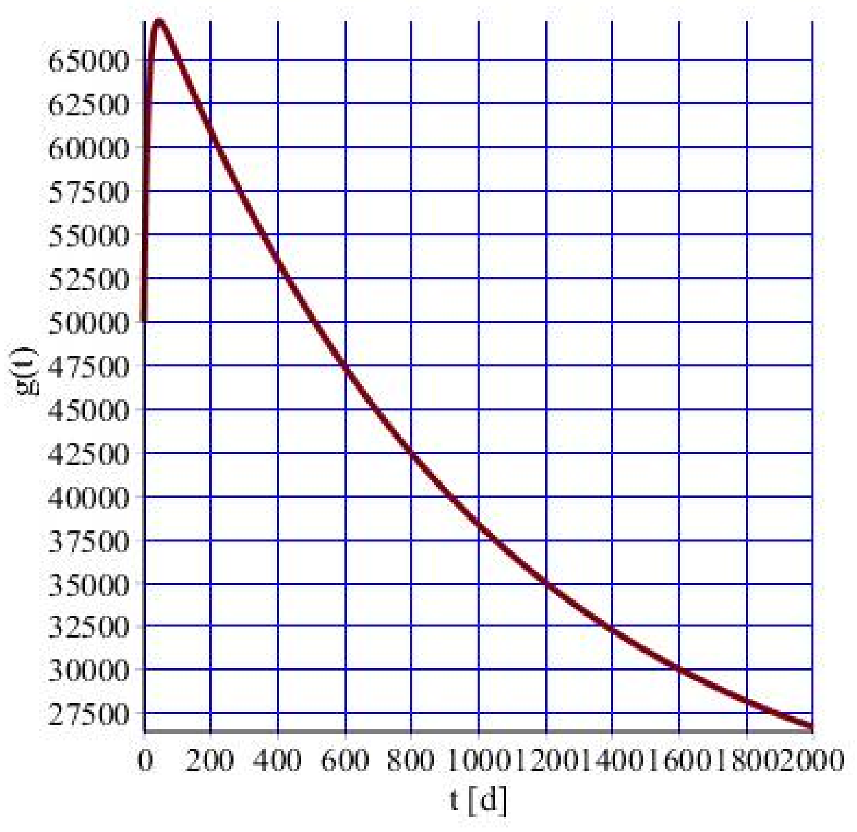
Results of simulation involving Equations (60)–(62) are reported in Figure 1, Figure 2 and Figure 3. Results of simulation regarding Equations (67)–(69) are shown in Figure 4 and Figure 5.
Figure 2 and Figure 4 represent concentration profiles of U234 at x = 0 for Robin and Dirichlet boundary conditions respectively. As it is possible to see, main difference is in the initial value at t = 0. It is important to notice that the limit for t tending to zero of Equation (67) when x = 0, does not satisfy boundary conditions: it is expected that concentration of U234 at x = 0 for t equal to zero equals g(0) for Dirichlet boundary conditions, so the solution in Equation (67) is valid for all x > 0.
Figure 3 and Figure 5 represent concentration of U234 at t = 100 years along x for the two models, according to radionuclide decay. The profile computed under Robin boundary conditions reaches a maximum in concentration at a certain x (Robin conditions well describe mass conservation) while at the same t the solution computed under Dirichlet boundary conditions shows lower values of concentration.
4. Conclusions
The contaminant transport in porous media has an important role in environmental engineering science, hydrology, geology, and petroleum engineering. Despite the fact that the Advection-Dispersion Equations describe the physical problem, it is difficult to derive analytical solutions if chemical processes also take place. Analytical solutions are helpful for testing numerical models and for screening level environmental risk assessment.
The 1D–model proposed in this paper and its analytical solution can be suitable to define tank or pipeline failure, or pollution by DNAPLs (Dense NonAqueous Phase Liquids) or by radioactive contaminants, because the source is described as a time dependent function with a combined contaminant production-consumption, and moreover, it is given as a Robin boundary condition. The comparison of the proposed solution with the closed form analytical solution obtained for a time dependent production-decay source expressed as a Dirichlet boundary condition shows that the use of the Dirichlet boundary condition can underestimate concentration profiles.
The analytical solution is consistent with previous ones, since it tends towards known solutions for certain values of the parameters (limit cases) and it can be derived from a more general one for some particular conditions at the source.
Author Contributions
Conceptualization, A.M. and O.P.; Methodology, R.C.; Software, A.M.; Supervision, O.P.; Validation, A.M., R.C. and O.P.; Writing—original draft, A.M. and O.P.
Funding
This research received no external funding.
Conflicts of Interest
The authors declare no conflict of interest.
Appendix A
Equation above gives the relationship between flux-averaged concentration Cf and volume-average concentration Cr [32,33,34].
In fact, by considering Equation (1) rewritten as:
Please note that the term in square brackets is zero.
By doing some passages we get:
By substituting Equation (A1) in Equation (A5) we get the following expression that is identical to Equation (1):
The substitution of Equation (A1) in third-type boundary conditions let passing to first-type boundary conditions as follows:
By considering Equation (21):
It follows from Equation (A1) that:
By substituting Equation (A7) in Equation (6) we obtain:
That is a first-type boundary condition in terms of flux-average concentration.
Finally, on the bases of the correlation between Cf and Cr that let to pass from third-type boundary conditions to first-type boundary conditions, it is possible to derive directly the first-type solution from the third-type solution and it will be consistent with mass conservation.
By considering Equation (26), the equivalent solution for first boundary conditions is:
where:
By doing some passages we obtain:
References
- Leij, F.J.; Skaggs, T.H.; van Genuchten, M.T. Analytical Solutions for Solute Transport in Three-Dimencional Semi-infinite Porous Media. Water Resour. Res. 1991, 27, 2719–2733. [Google Scholar] [CrossRef]
- Leij, F.J.; Toride, N.; van Genuchten, M.T. Analytical solutions for non-equilibrium solute transport in three-dimensional porous media. J. Hydrol. 1993, 151, 193–228. [Google Scholar] [CrossRef] [Green Version]
- Massabó, M.; Cianci, R.; Paladino, O. Some analytical solutions for two-dimensional convection-dispersion equation in cylindrical geometry. Environ. Model. Softw. 2006, 21, 681–688. [Google Scholar] [CrossRef]
- Chen, J.S.; Chen, J.T.; Liu, C.W.; Liang, C.P.; Lin, C.W. Analytical solutions to two-dimensional advection-dispersion equation in cylindrical coordinates in finite domain subject to first- and third-type inlet boundary conditions. J. Hydrol. 2011, 405, 522–531. [Google Scholar] [CrossRef]
- Cianci, R.; Massabó, M.; Paladino, O. An analytical solution of the advection dispersion equation in a bounded domain and its application to laboratory experiments. J. Appl. Math. 2011, 493014. [Google Scholar] [CrossRef]
- Fedi, A.; Massabò, M.; Paladino, O.; Cianci, R. A new analytical solution for the 2D advection-dispersion equation in semi-infinite and laterally bounded domain. Appl. Math. Sci. 2010, 4, 3733–3747. [Google Scholar]
- Van der Zee, S.E.A.T.M. Analysis of solute redistribution in a heterogeneous field. Water Resour. Res. 1990, 26, 273–278. [Google Scholar] [CrossRef]
- Bosma, W.J.P.; Van der Zee, S.E.A.T.M. Transport of reacting solute in a one-dimensional, chemically heterogeneous porous medium. Water Resour. Res. 1993, 29, 117–131. [Google Scholar] [CrossRef]
- Sagar, B. Dispersion in three dimensions: Approximate analytic solutions. ASCE J. Hydraul. Div. 1982, 108, 47–62. [Google Scholar]
- Yeh, H. AT123D: Analytical Transient Simulation of Waste Transport in the Aquifer System; Oak Ridge National Lab: Oak Ridge, TN, USA, 1981. [Google Scholar]
- Batu, V. A generalized two-dimensional analytical solution for hydrodynamic dispersion in bounded media with the first-type boundary condition at the source. Water Resour. Res. 1989, 25, 1125–1132. [Google Scholar] [CrossRef]
- Batu, V. A generalized two-dimensional analytical solute transport model in bounded media for flux-type finite multiple sources. Water Resour. Res. 1993, 29, 2881–2892. [Google Scholar] [CrossRef]
- Batu, V. A generalized 3-dimensional analytical solute transport model for multiple rectangular first-type sources. J. Hydrol. 1996, 174, 57–82. [Google Scholar] [CrossRef]
- Neville, J. Compilation of Analytical Solutions for Solute Transport in Uniform Flow; Papadopus & Associates: Bethesda, MD, USA, 1994. [Google Scholar]
- Suk, H. Developing semianalytical solutions for multispecies transport coupled with a sequential first-order reaction network under variable flow velocities and dispersion coefficients. Water Resour. Res. 2013, 49, 3044–3048. [Google Scholar] [CrossRef] [Green Version]
- Suk, H. Generalized semi-analytical solutions to multispecies transport equation coupled with sequential first-order reaction network with spatially or temporally variable transport and decay coefficients. Adv. Water Resour. 2016, 94, 412–423. [Google Scholar] [CrossRef]
- Leij, F.J.; Priesack, E.; Schaap, M.G. Solute transport modeled with Green’s functions with application to persistent solute sources. J. Contam. Hydrol. 2000, 41, 155–173. [Google Scholar] [CrossRef]
- Park, E.; Zhan, H. Analytical solutions of contaminant transport from finite one-, two-, and three-dimensional sources in a finite-thickness aquifer. J. Contam. Hydrol. 2001, 53, 41–61. [Google Scholar] [CrossRef]
- Wang, H.; Wu, H. Analytical solutions of three-dimensional contaminant transport in uniform flow field in porous media: A library. Front. Environ. Sci. Eng. China 2009, 3, 112–128. [Google Scholar] [CrossRef]
- Yeh, G.T.; Tsai, Y.J. Analytical three dimensional transient modelling of effluent discharges. Water Resour. Res. 1976, 12, 533–540. [Google Scholar] [CrossRef]
- Martin-Hayden, J.M.; Robbins, G.A. Plume Distortion and Apparent Attenuation Due to Concentration Averaging in Monitoring Wells. Ground Water 1997, 35, 339–346. [Google Scholar] [CrossRef]
- Paladino, O.; Moranda, A.; Massabò, M.; Robbins, G.A. Analytical Solutions of Three-Dimensional Contaminant Transport Models with Exponential Source Decay. Groundwater 2018, 56, 96–108. [Google Scholar] [CrossRef] [PubMed]
- Sanskrityayn, A.; Suk, H.; Kumar, N. Analytical solutions for solute transport in groundwater and riverine flow using Green’s Function Method and pertinent coordinate transformation method. J. Hydrol. 2017, 547, 517–533. [Google Scholar] [CrossRef]
- Chen, J.S.; Li, L.Y.; Lai, K.H.; Liang, C.P. Analytical model for advective-dispersive transport involving flexible boundary inputs, initial distributions and zero-order productions. J. Hydrol. 2017, 554, 187–199. [Google Scholar] [CrossRef]
- Van Genuchten, M.T.; Alves, W.J. Analytical Solutions of the One-Dimensional Convective-Dispersive Solute Transport Equation; United States Department of Agriculture, Economic Research Service: Washington, DC, USA, 1982.
- Pérez Guerrero, J.S.; Pontedeiro, E.M.; van Genuchten, M.T.; Skaggs, T.H. Analytical solutions of the one-dimensional advection-dispersion solute transport equation subject to time-dependent boundary conditions. Chem. Eng. J. 2013, 221, 487–491. [Google Scholar] [CrossRef]
- Clement, T.P. Generalized solution to multispecies transport equations coupled with a first-order reaction network. Water Resour. Res. 2001, 37, 157–163. [Google Scholar] [CrossRef] [Green Version]
- Srinivasan, V.; Clement, T.P. Analytical solutions for sequentially coupled one-dimensional reactive transport problems—Part I: Mathematical derivations. Adv. Water Resour. 2008, 31, 203–218. [Google Scholar] [CrossRef]
- Srinivasan, V.; Clement, T.P. Analytical solutions for sequentially coupled one-dimensional reactive transport problems—Part II: Special cases, implementation and testing. Adv. Water Resour. 2008, 31, 219–232. [Google Scholar] [CrossRef]
- Catania, F.; Massabò, M.; Paladino, O. Estimation of transport and kinetic parameters using analytical solutions of the 2D advection-dispersion-reaction model. Environmetrics 2006, 17, 199–216. [Google Scholar] [CrossRef]
- Batu, V.; van Genuchten, M.T. First- and third-type boundary conditions in two-dimensional solute transport modeling. Water Resour. Res. 1990, 26, 339–350. [Google Scholar] [CrossRef]
- Brigham, W.E. Mixing Equations in Short Laboratory Cores. Soc. Pet. Eng. J. 1974, 14, 91–99. [Google Scholar] [CrossRef]
- Parker, J.C.; van Genuchten, M.T. Flux-Averaged and Volume-Averaged Concentrations in Continuum Approaches to Solute Transport. Water Resour. Res. 1984, 20, 866–872. [Google Scholar] [CrossRef]
- Kreft, A.; Zuber, A. On the physical meaning of the dispersion equation and its solutions for different initial and boundary conditions. Chem. Eng. Sci. 1978, 33, 1471–1480. [Google Scholar] [CrossRef]
- Kreft, A.; Zuber, A. On the use of the dispersion model of fluid flow. Int. J. Appl. Radiat. Isot. 1979, 30, 705–708. [Google Scholar] [CrossRef]
- Van Genuchten, M.T.; Parker, J.C. Boundary Conditions for Displacement Experiments Through Short Laboratory. Soil Columns. Soil Sci. Soc. Am. J. 1984, 48, 703–708. [Google Scholar] [CrossRef]
- Cho, C.M. Convective transport of ammonium with nitrification in soil. Can. J. Soil Sci. 1971, 51, 339–350. [Google Scholar] [CrossRef]
- Van Genuchten, M.T. Convective-dispersive transport of solutes involved in sequential first-order decay reactions. Comput. Geosci. 1985, 11, 129–147. [Google Scholar] [CrossRef]
- Chen, J.S.; Liu, C.W.; Liang, C.P.; Lai, K.H. Generalized analytical solutions to sequentially coupled multi-species advective-dispersive transport equations in a finite domain subject to an arbitrary time-dependent source boundary condition. J. Hydrol. 2012, 456–457, 101–109. [Google Scholar] [CrossRef]
- Higashi, K.; Pigford, H.T. Analytical Models for Migration of Radionuclides in Geologic Sorbing Media. J. Nucl. Sci. Technol. 1980, 17, 700–7009. [Google Scholar] [CrossRef]
Figure 1.
Boundary condition.

Figure 2.
Concentration profile at x = 0.

Figure 3.
Concentration profile at t = 5110 [d].

Figure 4.
Concentration profile at x = 0.

Figure 5.
Concentration profile at t = 5110 [d].


Table 1.
Radionuclide decay parameters.
| Parameters | 234U |
|---|---|
| Velocity, v [m year−1] | 100 |
| Dispersion coefficient [m2 year−1] | 4000 |
| First order decay constant λ [year−1] | 0.0000028 |
| Production constant λp [year−1] | 0.079 |
| Source decay constant λs [year−1] | 0.0010028 |
| Initial concentration of [mg m3] | 5 × 10⁴ |
© 2018 by the authors. Licensee MDPI, Basel, Switzerland. This article is an open access article distributed under the terms and conditions of the Creative Commons Attribution (CC BY) license (http://creativecommons.org/licenses/by/4.0/).
Share and Cite
MDPI and ACS Style
Moranda, A.; Cianci, R.; Paladino, O. Analytical Solutions of One-Dimensional Contaminant Transport in Soils with Source Production-Decay. Soil Syst. 2018, 2, 40. https://doi.org/10.3390/soilsystems2030040
AMA Style
Moranda A, Cianci R, Paladino O. Analytical Solutions of One-Dimensional Contaminant Transport in Soils with Source Production-Decay. Soil Systems. 2018; 2(3):40. https://doi.org/10.3390/soilsystems2030040
Chicago/Turabian StyleMoranda, Arianna, Roberto Cianci, and Ombretta Paladino. 2018. "Analytical Solutions of One-Dimensional Contaminant Transport in Soils with Source Production-Decay" Soil Systems 2, no. 3: 40. https://doi.org/10.3390/soilsystems2030040