A Molecular Investigation of Soil Organic Carbon Composition across a Subalpine Catchment

Abstract

The dynamics of soil organic carbon (SOC) storage and turnover are a critical component of the global carbon cycle. Mechanistic models seeking to represent these complex dynamics require detailed SOC compositions, which are currently difficult to characterize quantitatively. Here, we address this challenge by using a novel approach that combines Fourier transform infrared spectroscopy (FT-IR) and bulk carbon X-ray absorption spectroscopy (XAS) to determine the abundance of SOC functional groups, using elemental analysis (EA) to constrain the total amount of SOC. We used this SOC functional group abundance (SOC-fga) method to compare variability in SOC compositions as a function of depth across a subalpine watershed (East River, Colorado, USA) and found a large degree of variability in SOC functional group abundances between sites at different elevations. Soils at a lower elevation are predominantly composed of polysaccharides, while soils at a higher elevation have more substantial portions of carbonyl, phenolic, or aromatic carbon. We discuss the potential drivers of differences in SOC composition between these sites, including vegetation inputs, internal processing and losses, and elevation-driven environmental factors. Although numerical models would facilitate the understanding and evaluation of the observed SOC distributions, quantitative and meaningful measurements of SOC molecular compositions are required to guide such models. Comparison among commonly used characterization techniques on shared reference materials is a critical next step for advancing our understanding of the complex processes controlling SOC compositions.

1. Introduction

Soil organic carbon (SOC) represents the largest terrestrial carbon reservoir in contact with the atmosphere [1]. However, cycling of carbon through soils is one of the least understood components of the global carbon cycle [2,3,4,5]. In particular, the mechanisms for and timescales over which SOC responds to environmental changes are imprecisely known [2]. As a result, predictions from process-based terrestrial biosphere models show considerable variability and limited agreement with experimental measurements [4]. Therefore, SOC represents a key uncertainty in model predictions of land surface responses to global warming. Recent studies have shown that the traditional representations of SOC based on chemical recalcitrance are inconsistent with the observed SOC molecular structures [2,6]. Further, such representations do not capture the physical protection and differential SOC temperature sensitivity associated with biotic and abiotic controls on SOC turnover [7,8,9,10]. In order to advance SOC research and increase our confidence in predictions of soil feedbacks in response to changing climate conditions, there is an urgent need to improve our mechanistic understanding of SOC turnover and stabilization [2,11].

To contribute towards our mechanistic understanding of SOC turnover and stabilization, we quantitatively evaluate SOC compositions across a subalpine watershed at East River, Colorado, USA. The quantification of SOC composition has long been a challenging task. For over 200 years, alkaline extraction has been used for SOC isolation and characterization, but SOC often cannot be completely extracted (30–50% yield), and harsh alkaline treatments can hydrolyze SOC that is stable within the typical soil pH range (3.5–8.5) [7]. Therefore, soil extracts often do not accurately reflect the SOC composition of bulk soils in nature. Most mass spectrometry (MS) techniques and liquid-state ¹³C nuclear magnetic resonance (NMR) spectroscopy require the extraction of soil samples [12]. Pyrolysis gas chromatography (py-GC) MS does not require extraction, but the artificial breakdown of large SOC molecules and varied ionizability between different types of SOC molecules complicate the quantification of SOC [12,13]. Solid state cross polarization-magnetic angle spinning (CP-MAS) ¹³C NMR often requires HF_(aq) treatment to remove magnetic particles and concentrate carbon, especially in soils with low carbon content, which in turn alters the soil samples being studied [14,15,16,17,18]. Previous studies show mixed results on whether HF_(aq) treatment changes the distribution of SOC [19,20], which can also complicate SOC quantification. Further, low ¹³C natural abundance and variations in the nuclear Overhauser effect (NOE) from proton decoupling of different types of carbon atoms may make SOC quantification using ¹³C NMR spectroscopy more difficult [21]. To avoid complexity arising from chemical treatments and to improve our quantitative understanding of SOC, we applied complementary spectroscopic techniques on bulk soils to study SOC composition with minimal perturbation.

Fourier transform infrared spectroscopy (FT-IR) and bulk carbon X-ray absorbance spectroscopy (XAS) are powerful tools to identify organic functional groups in bulk soils [22,23]. However, FT-IR and bulk C XAS are only semi-quantitative, relying on a relative comparison of peak areas [23,24]. Further, while FT-IR is sensitive to aliphatic C–H stretches, amide C=O stretches, and carbonyl C=O stretches, it is not as sensitive to the C=C bond stretches dominant in plant materials and other complex aromatic structures in soil. Additionally, the IR absorbance of polysaccharide-like molecules overlaps with minerals, making the peaks difficult to resolve. Therefore, in this study, we used FT-IR to identify carbonyl, amide, and aliphatic functional groups. Aliphatic C–H has symmetric (2800–2900 cm⁻¹) and asymmetric (2900–3000 cm⁻¹) stretches, and an amide bond has amide I (C=O stretch, 1600–1630 cm⁻¹) and amide II (N–H bend and C=N stretch, 1500–1590 cm⁻¹) [23]. In this study, we only used the symmetric C–H stretch and the stronger amide I band to avoid overestimating the amount of aliphatic and amide (

Table 1. Soil organic carbon (SOC) functional groups and corresponding techniques.

Functional Group	Technique	Absorption Energy
Carbonyl	FT-IR	1700–1800 cm−1
Aliphatic		2800–3000 cm−1 (symmetric)
Amide		1630–1660 cm−1 (amide I)
Quinonic	Bulk C XAS	283–284.9 eV
Aromatic		285.0–285.8 eV
Phenolic		286.0–287.4 eV
O-alkyl		289.2–289.5 eV

).

Bulk C XAS is sensitive to quinonic, aromatic, phenolic, and O-alkyl (polysaccharide-like) molecules, but it can be challenging to resolve amide, carboxylate, and aliphatic groups that all absorb between 287.0 and 288.7 eV [24,25,26]. Therefore, we used bulk C XAS to identify quinonic, aromatic, phenolic, and O-alkyl functional groups in soils in this study (Table 1). We applied each technique to identify the functional groups to which it is the most sensitive and combined the results using a linear mass balance model, where total organic carbon (TOC) measured by elemental analysis (EA) constrained the sum of organic functional groups measured from FT-IR and bulk C XAS. Because this linear mass balance fit approach is used to quantitatively evaluate the abundance of SOC functional groups, we refer to this method as the SOC functional group abundance (SOC-fga) method. To provide information about how SOC functional groups vary as a function of depth and landscape position, we apply the SOC-fga method to soil profiles from hillslope sites at two different elevations and from different landscape positions at each elevation across the East River watershed in Colorado, USA.

2. Materials and Methods

2.1. Field Sites Description, Sample Collection, and Preparation

Soil and selected plant and litter samples were collected from a hillslope site (Bradley Creek Meadow, BCM), a downslope depositional zone characterized by a higher soil moisture (Bradley Creek Willow, BCW), a higher-elevation hillslope meadow (Rock Creek Meadow, RCM), and a downslope groundwater-fed fen (Rock Creek Fen, RCF) (

Table 2. Field sites description.

Site	Coordinates	Elevation (m)	Description	Soil Series/Subgroup	AGB (g/m2)	Average Temperature (°C)
BCM	38°59′12.4″ N, 107°00′11.06″ W	2987	Subalpine meadow vegetation on hillslope dominated by perennial forbs (ca. 80%), graminoids (ca. 15%), litter (3%), and bare soil (2%).	Leaps silty clay loam/Typic Cryoborolls	331.10	6.9 (30 cm); 6.5 (100 cm)
BCW	38°59′15.10″ N, 107°00′14.10″ W	2975	Small drainage adjacent to BCM covered by a mixture of willow (Salix spp.), graminoids, and perennial forbs.	Leaps silty clay loam/Typic Cryoborolls	not determined	5.0 (30 cm); 5.3 (100 cm)
RCM	38°58′46.37″ N, 107°02′16.96″ W	3466	Subalpine meadow vegetation with 100% perennial forbs.	Bucklon silt loam/Typic Cryoborolls	824.41	3.8 (30 cm); 3.7 (100 cm)
RCF	38°58′57.76″ N, 107°01′49.32″ W	3444	Willow (Salix spp.)-dominated groundwater fen adjacent to a small stream.	No series affiliatio/Histic Cryaquolls	not determined	not determined

BCM: Bradley Creek Meadow; BCW: Bradley Creek Willow; RCM: Rock Creek Meadow; RCF: Rock Creek Fen; AGB: Above-ground biomass.

). Based on the U.S. Geological Survey (USGS) 10 m digital elevation model (DEM), BCM has a slope of 10° and aspect of 240°; BCW has a slope of 3° and aspect of 185°; RCM has a slope of 8° and aspect of 115°; and RCF has a slope of 3° and aspect of 140°.

All sites are within the East River Basin, a shale-dominated watershed associated with the Rocky Mountain Biological Laboratory (RMBL), Crested Butte, CO. One soil core was collected from each site by hand auguring to saprolite, which is weathered Mancos Shale at all study sites. The depth increments of the cores were chosen to reflect an approximately 10-cm increments. Soil samples were then bagged, labeled, air-dried, sieved to collect the <2 mm fractions, and ground to fine powder with agate mortar and pestle for all characterization experiments. Above-ground biomass (AGB) collected from 1.3 × 1.3 m² areas at BCM and RCM along with litter and select plant samples from each site were dried at 60 °C for 2–3 days to constant mass and homogenized and ground to <0.4 mm with a metal blade for all characterization experiments.

Fractional plant cover was estimated at the meadow sites using a 13 × 13 grid of 1.3 m × 1.3 m in August 2016. The fractional cover at both sites is the average of five randomly distributed surveys within 50 m of the soil sampling site. Fractional plant cover was not estimated at BCW and RCF because the quadrant approach cannot be used where (Salix spp.) dominates. All sites in this study are grazed during the fall season, but based on our qualitative observations, the grazing pressure at BC is consistently more intense than at RCM or RCF. Therefore, we expect a greater reduction in above-ground plant inputs but an enhanced input of cattle excrement at BCM and BCW.

To monitor soil environmental conditions, depth-arrays of soil temperature and water content reflectometer probes (CS655, Campbell Scientific, Logan, UT, USA) were installed at BCW (November 2015), BCM (June 2016), and RCM (June 2016). Sensors were installed horizontally in soil pits at depths ranging from 10 cm to 130 cm. Soil temperature and volumetric water content (VWC) from each depth were logged at 1 to 6 h intervals. For the purpose of this study, only the shallow (30 cm) and deep (100 cm) soil data across BCW, BCM, and RCM are compared.

2.2. Elemental Analysis

Elemental analysis (EA) was used to measure bulk soil C and N content. Measurements were preformed using the Carlo-Erba NA 1500 analyzer (Thermo Fisher Scientific, Waltham, MA, USA) at the Environmental Measurements Facility (EM1) at Stanford University. To measure the total nitrogen (TN) and total carbon (TC) of the samples, 20–30 mg of ground soil samples or 3–4 mg of biomass samples were weighed into tin capsules and loaded into the analyzer. A method previously published was used to measure total organic carbon (TOC) and total inorganic carbon (TIC) by HCl_(aq) treatment [27]. Briefly, 400 mg of ground soil sample was added to a scintillation vial. Then, 4 mL of 3 M HCl_(aq) was slowly added to the vial via a pipette to remove inorganic carbonate, and the vial was capped loosely. The vial was swirled occasionally for 15 min and the cap was removed to displace accumulated CO₂. After the weight of the solution in the vial stopped changing, the solution was centrifuged to remove the supernatant, and the soil pellet was washed with deionized (DI) water (10 mL × 2). Afterwards, the soil pellet was air-dried and ground with agate mortar and pestle, then 20–30 mg of ground soil sample was weighed into tin capsules and injected into the analyzer to measure the remaining TOC. TIC was calculated by subtracting TOC from TC.

2.3. Fourier Transform Infrared Spectroscopy (FT-IR)

All FT-IR measurements were performed on the Nicolet iS50 FT-IR spectrometer (Thermo Fisher Scientific, Waltham, MA, USA) at the Soft and Hybrid Materials Facility (SMF) at Stanford Nano Shared Facilities (SNSF). First, 5–10 mg of ground soil samples or 2–3 mg of biomass sample was loaded directly onto the attenuated total reflectance (ATR) detector with a spatula to obtain the IR spectrum for each sample. A method previously published was used to obtain the mineral-enriched background for soils by chemical treatment [28]. Briefly, 100 mg of ground soils sample was mixed with 0.625 mL of NaOCl_(aq) (6% w/w, pH = 9.5) and incubated at 80 °C for 15 min to allow for the oxidation of organic compounds. The solution was centrifuged and the supernatant was discarded. The treatment was repeated a total of three times. The soil pellet was then washed with deionized (DI) water (10 mL × 2), air-dried, and ground with an agate mortar and pestle. Afterwards, 5–10 mg of ground soil sample was loaded directly onto the ATR detector with a spatula to obtain the mineral-enriched background spectrum. The mineral background was subtracted from the bulk soil spectrum to obtain the SOC spectrum. Peak deconvolution was performed with the Igor Pro software package (version 7, WaveMetrics Inc., Portland, OR, USA). The peak deconvolution parameters are listed in

Table 3. Fitting parameters for FT-IR spectra using the Igor Pro software package.

Parameter	Values
Noise level	10−5–10−4
Smooth factor	10–55
Min fraction	0.05
Peak shape	Gauss

(please see Supplementary Materials Figures S1 and S2 for examples of deconvoluted spectra).

2.4. Bulk C X-ray Absorption Spectroscopy (XAS)

All bulk C XAS data were collected on the SGM beam line (11ID-1) at the Canadian Light Source (CLS), Saskatoon, Canada. Sample preparation was done according to a procedure that was published previously [22]. Briefly, for each bulk XAS sample, 10 mg of ground soil or 5 mg of biomass was added to 0.1 mL of DI water in a 0.8 mL snap-cap eppendorf tube. The tube was capped and the solution was mixed on a vortex mixer for 5 s. Then, 8–10 μL of the suspended soil solution was drop-deposited onto a gold-coated silicon wafer and air-dried. The wafers were prepared by the CLS staff by heating gold pellets above 650 °C in a vacuum chamber containing the silicon wafers. Bulk C XAS spectra were collected over the range of 270–320 eV with 0.1 eV intervals. One fast (slew) scan was performed on 60 different spots on each sample to minimize beam damage, and the 60 scans were averaged into the final spectrum. Total partial fluorescence yield (PFY) counts of all spectra (10–15 kpc) were well below the detector saturation limit (20–30 kpc). Peak deconvolution was performed with the Athena software package (version 0.9.25, Bruce Ravel). The peak fitting parameters are listed in

Table 4. Fitting parameters for bulk C XAS spectra using the Athena software package.

Parameter	Values
Edge normalization	I0 = 290 eV
Edge step	1
Pre-edge	270–280 eV
Post-edge	310–318 eV
Gaussian FWHM	0.3–0.5
Sigma* FWHM	3
Arctangent width	0.3
Arctangent height	1–3 (depending on the height of the K-edge)
Peak shape	Gauss

FWHM = full width at the half maximum of a peak.

, and the energy for each functional group was assigned based on the literature [25] (please see Supplementary Materials Figures S3 and S4 for examples of fitted spectra).

2.5. X-ray Fluorescence (XRF) Spectrometry

XRF was used to measure the elemental components of soil samples. All XRF data were collected from the Spectro Xepos HE XRF spectrometer (Spectro Analytical Instruments, Kleve, Germany) at EM1. To prepare the samples, 3 g of ground soil was loaded into a plastic sample cup, and the cup was sealed with polypropylene film. The plastic cups were loaded into the spectrometer for measurement. Data analysis was performed automatically by the Spectro Xepos software (Spectro Analytical Instruments, Kleve, Germany). XRF data are included in Supplementary Materials.

2.6. Powder X-ray Diffraction (PXRD)

PXRD was used to determine the mineral compositions of soil samples. All PXRD data were collected from the Rigaku MiniFlex 600 Benchtop X-Ray Diffraction System (Rigaku Corporation, Tokyo, Japan) at EM1. To prepare the samples, 100 mg of ground soil was added to a snap-cap Eppendorf tube, and 1 mL of isopropyl alcohol was added to the soil. The tube was capped and the solution was mixed for 30 s with a vortex mixer. Then, 200 μL of solution was drop-deposited onto a crystal quartz sample holder and air-dried. Soil samples were loaded into the diffractometer with the X-ray generator set to 40 kV and 15 mA. Data were collected at 2θ = 3°–90° with 0.01° intervals. PXRD data are included in Supplementary Materials.

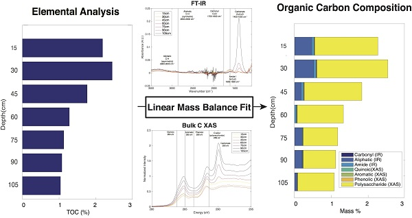
2.7. Linear Mass Balance Model to Quantify SOC Functional Group Abundance (SOC-fga Method)

We developed a method that combines FT-IR and bulk C XAS results to quantify SOC functional group abundance (the SOC-fga method) using the Beer–Lambert Law:

$$A=d\times \epsilon \times b\times c,$$

(1)

where A is absorbance (peak area), d is a scalar accounting for the peak area ratio between FT-IR and bulk C XAS, ε is the molar absorption coefficient that depends on various factors, including wavelength, compound, soil matrix, pH, and instrumentation, b is the path length of the light beam through a sample, and c is the analyte concentration [29,30,31]. The concentration of SOC species can be expressed as:

$$c=\frac{mol{e}_{SOC}}{volum{e}_{soil}}=\frac{\frac{mas{s}_{SOC}}{M{W}_{SOC}}\times densit{y}_{soil}}{mas{s}_{soil}}=\frac{mass{\%}_{SOC}\times densit{y}_{soil}}{M{W}_{SOC}},$$

(2)

where MW_SOC is the molecular weight of the SOC species of interest.

Equation (1) can be written as:

$$\frac{A}{n}=\frac{d\times \epsilon \times b\times mass{\%}_{SOC}\times densit{y}_{soil}}{M{W}_{SOC}}$$

(3)

where n is the number of functional groups in each compound (for example, if there are 300 amide bonds in a protein, n = 300).

The mass% of an SOC functional group of interest can therefore be expressed as:

$$mass{\%}_{SOC}=\frac{A\times M{W}_{SOC}}{n\times d\times \epsilon \times b\times densit{y}_{soil}}.$$

(4)

In Equation (4), A and density_soil were measured experimentally. Variables d and b are constant for the same instrument (FT-IR or bulk C XAS). Variables MW_SOC, n, and ε are different between different functional groups. For simplicity, we assumed that MW_SOC, n, and ε for a functional group are constant for soils from the same site because they are likely to have similar SOC input and soil matrices. Variables that are constant (d, b) or assumed to be constant for each functional group (MW_SOC, n, ε) were grouped into an arbitrary variable, α_i, where i is an index representing the functional group (i.e., carbonyl, aliphatic, amine, quinonic, aromatic, phenolic, or polysaccharide):

$${\alpha }_i=\frac{M{W}_i}{n_i\times d\times {\epsilon }_i\times b}$$

(5)

such that mass% can be rewritten as:

$$mass{\%}_i=\frac{A_i\times {\alpha }_i}{densit{y}_{soil}}.$$

(6)

Assuming FT-IR and bulk C XAS together detect all SOC functional groups, experimentally measured TOC is the sum of mass% of all SOC functional groups identified:

$$TOC\left(mass\%\right)={\displaystyle \sum }_{i}mass{\%}_i={\displaystyle \sum }_i\frac{A_i\times {\alpha }_i}{densit{y}_{soil}}.$$

(7)

We identified seven important organic functional groups (Table 1), such that Equation (7) has seven unknown α_i values, requiring at least seven samples to constrain the system, represented in matrix form as:

$$\begin{array}{c}1\\ 2\\ 3\\ 4\\ 5\\ 6\\ 7\\ 8\\ 9\\ 10\\ ⋮\end{array}\left[\begin{array}{ccccccc}\frac{A_{C=O}^1}{{density}_{soil}^1}& \frac{A_{{CH}_3}^1}{{density}_{soil}^1}& \frac{A_{NC=O}^1}{{density}_{soil}^1}& \frac{A_{quin}^1}{{density}_{soil}^1}& \frac{A_{arom}^1}{{density}_{soil}^1}& \frac{A_{phen}^1}{{density}_{soil}^1}& \frac{A_{O-alkyl}^1}{{density}_{soil}^1}\\ \frac{A_{C=O}^2}{{density}_{soil}^2}& & & & & & \\ \frac{A_{C=O}^3}{{density}_{soil}^3}& & & & & & \\ \frac{A_{C=O}^4}{{density}_{soil}^4}& & & & & & \\ \frac{A_{C=O}^5}{{density}_{soil}^5}& & & & & & \\ \frac{A_{C=O}^6}{{density}_{soil}^6}& ⋮& ⋮& ⋮& ⋮& ⋮& ⋮\\ \frac{A_{C=O}^7}{{density}_{soil}^7}& & & & & & \\ \frac{A_{C=O}^8}{{density}_{soil}^8}& & & & & & \\ \frac{A_{C=O}^9}{{density}_{soil}^9}& & & & & & \\ \frac{A_{C=O}^{10}}{{density}_{soil}^{10}}& & & & & & \\ ⋮& & & & & & \end{array}\right]\times \left[\begin{array}{c}{\alpha }_{C=O}\\ {\alpha }_{{CH}_3}\\ {\alpha }_{NC=O}\\ {\alpha }_{quin}\\ {\alpha }_{arom}\\ {\alpha }_{phen}\\ {\alpha }_{O-alkyl}\end{array}\right]=\left[\begin{array}{c}{TOC}^1\\ {TOC}^2{TOC}^3\\ {TOC}^4\\ {TOC}^5\\ {TOC}^6\\ {TOC}^7\\ {TOC}^8\\ {TOC}^9\\ {TOC}^{10}\\ ⋮\end{array}\right],$$

(8)

where A^j_i is the peak area measurement for sample j and functional group i, and the experimentally measured TOC^j for sample j is used for the optimization for α_i. The calculated α_i values are thus applicable to all samples from the same site and can be used to calculate mass%_i. We used the linear least squares function in Matlab’s optimization toolbox to optimize the α_i vector in Equation (8) (boundary condition: α_i ≥ 0.01) for Bradley Creek (BCM and BCW), RCM, RCF, and above-ground biomass (AGB) separately (see Supplementary Materials Figures S5–S13 and Tables S1–S3 for comparison among different sample groupings in Equation (8), Figure S14 and Tables S4–S5 for uncertainties, and Figure S15 and Tables S6–S8 for boundary conditions). The optimized α_i vector is unique provided that the number of data points (soil samples) is larger than or equal to the number of unknowns (seven functional groups). The R² values between experimentally measured TOC and optimized TOC were used to evaluate how well the two sets of TOC values correlate to each other and how good the fits are.

The seven functional groups identified in this work, although comprehensive, are not direct representations of organic molecules because some molecules have multiple functional groups. For example, a lignin molecule can have aromatic, aliphatic, and O-alkyl functional groups. This could be a source of error, and therefore slope t-tests were performed to determine collectively whether the deviation of optimized TOC from experimentally measured TOC is significant (see Supplementary Materials Tables S1 and S7 for slope t-test).

2.8. Comparison between the SOC-fga Method and Individual Spectroscopic Techniques

To assess the differences between using peak areas from a single spectroscopic technique for Equation (8) and the SOC-fga method, where peak areas from both FT-IR and bulk C XAS are used, we compared the agreement between measured TOC and the optimized sum of organic carbon functional groups from Equation (8) using peak areas from individual techniques as well as the SOC-fga method. To ensure that seven functional groups are used for fits using all three methods, additional peaks were assigned in IR and bulk C XAS spectra. For FT-IR, the following peaks were identified in addition to the IR peaks listed in Table 1, and the peak areas were used in Equation (8): polysaccharide (1000–1160 cm⁻¹), phenolic (1380–1410 cm⁻¹), aromatic (1500–1550 cm⁻¹), and quinonic (1650 cm⁻¹) [23]. For bulk C XAS, the following peaks were identified in addition to the XAS peaks listed in Table 1, and the peak areas were used in Equation (8): aliphatic (287.45 eV), amide (288.45 eV), and carbonyl (290.3 eV). For the SOC-fga method, only the peaks listed in Table 1 were used in Equation (8). In the absence of standard soils with known SOC composition to further validate the linear mass balance fit model, the SOC mass% calculated using the SOC-fga method was used as the reference (percent difference = 0), and the percent difference for using either FT-IR or XAS for Equation (8) was calculated by:

$$percentdifference=\frac{mass{\%}_i^k-mas{s}_i^{SOC-fga}}{mas{s}_i^{SOC-fga}},$$

(9)

where k represents either FT-IR or bulk C XAS, and i represents a functional group (i.e., carbonyl, aliphatic, amide, quinonic, aromatic, phenolic, or polysaccharide).

3. Results

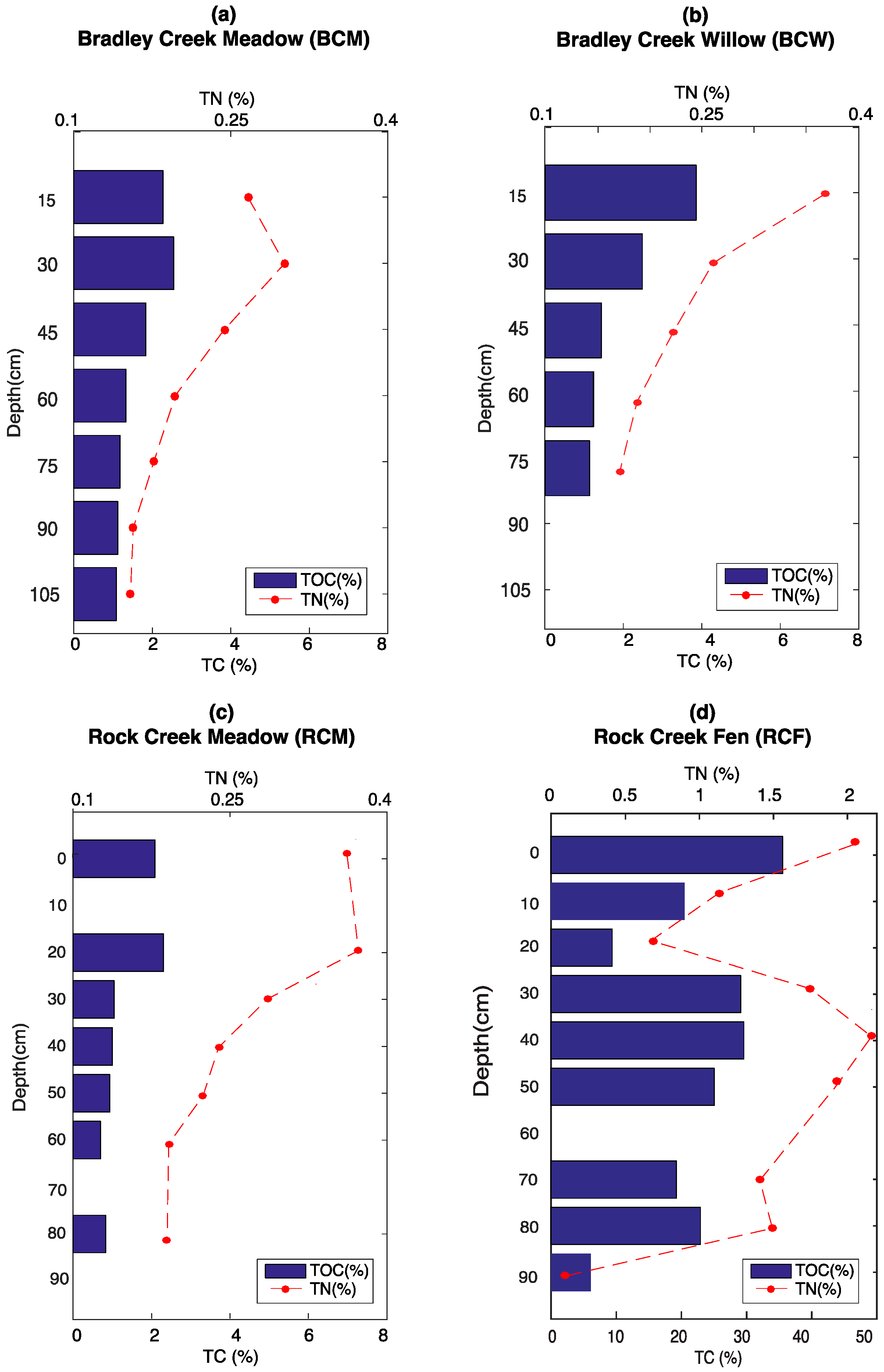
3.1. Elemental Analysis

Total nitrogen (TN) and TOC decreases with depth at BCM, BCW, and RCM, as organic inputs associated with biological activity are the most abundant at the surface (Figure 1a–c). BCM, BCW, and RCM have a fairly similar TN and TOC concentration. The trends for TN and TOC at RCF through depth are not as simple (Figure 1d), but TN and TOC still co-vary with each other similar to the other three sites.

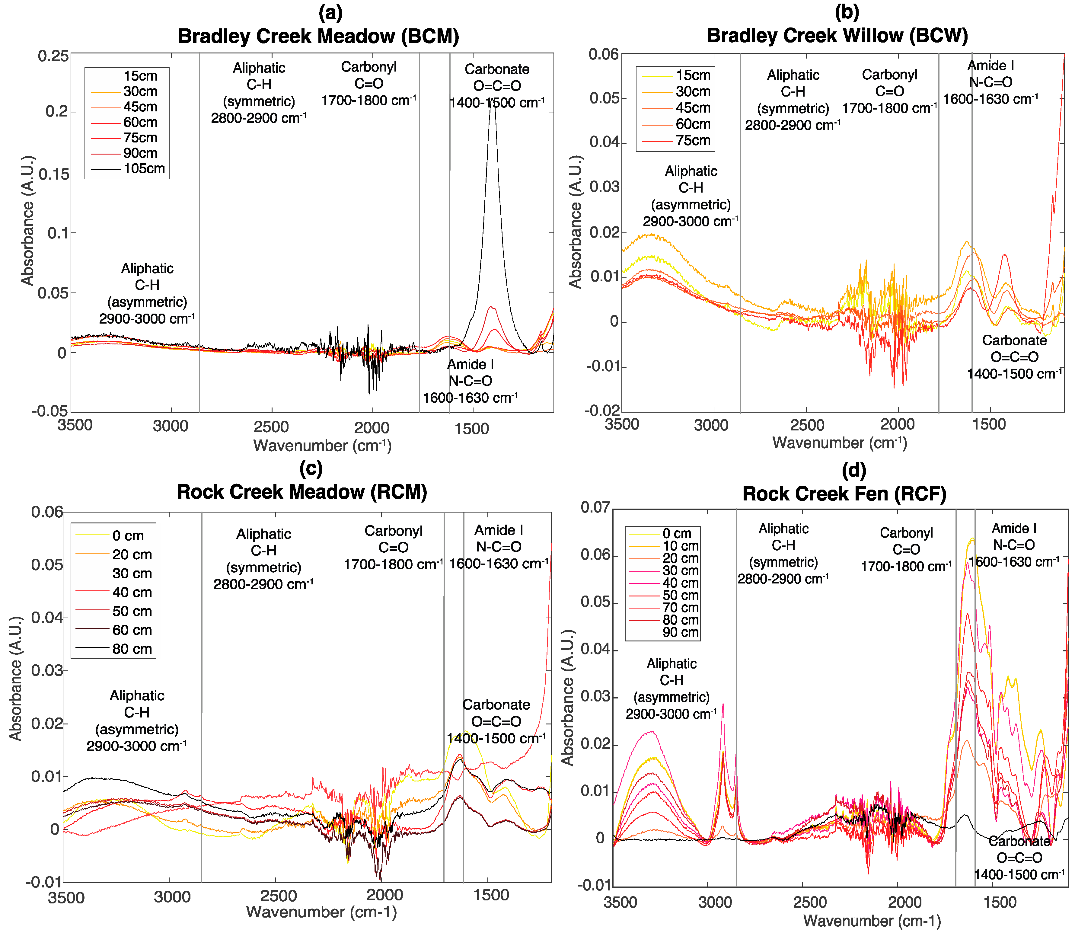
3.2. FT-IR Spectroscopy

FT-IR spectroscopy was used to identify carbonyl, amide, and aliphatic groups. The peak centroids used for the SOC-fga method are indicated with vertical lines in Figure 2. The spectral line shape of soils from the same site is relatively similar across depth but varies between sites, possibly due to variations in soil matrices between different sites. At BCM (Figure 2a), distinct carbonate peaks at 1400 cm⁻¹ are observed in samples deeper than 60 cm. This is consistent with total inorganic carbon (TIC) measured by EA, likely associated with carbonate (see SI, Figure S16). No carbonyl peak was observed, and aliphatic peak area decreases with depth overall. The amide peak area also generally decreases with depth, which is consistent with decreasing TN (Figure 1), given that over 90% of soil nitrogen is organic [32,33,34]. Carbonyl, aliphatic, and amide show similar trends at BCW but the carbonate peaks intensities are much lower (Figure 2b).

At RCM (Figure 2c), carbonyl peaks are present in the top 30 cm and aliphatic peak areas are relatively consistent through the top 60 cm, whereas the peak area of amide decreases with depth. At RCF (Figure 2d), the depth trends of peak areas for organic functional groups are not as obvious as at the other sites. On average, the peak areas of amide and carbonyl at RCM are larger than those in BCM and BCW. In addition, the relative peak intensities of aliphatic, amide, and carbonyl are much higher in RCF compared to the other three sites, consistent with the higher TOC at RCF.

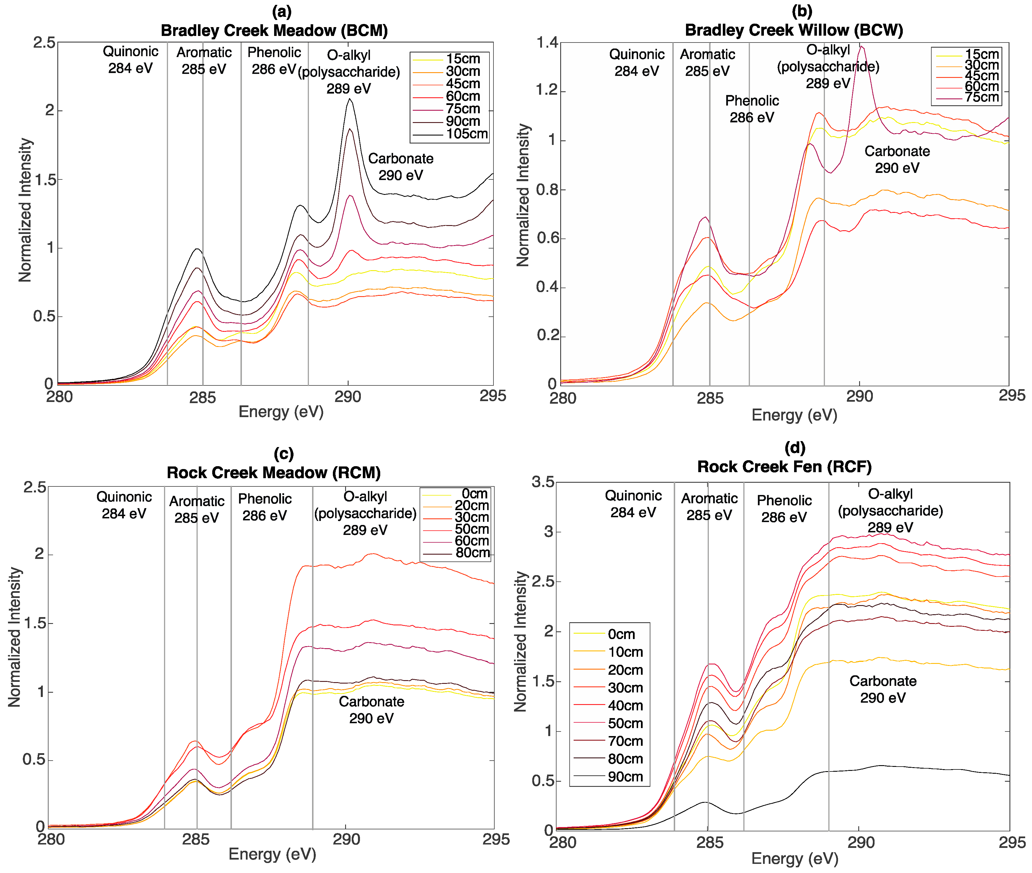
3.3. Bulk C XAS Spectroscopy

Bulk C XAS was used to identify quinonic, aromatic, phenolic, and O-alkyl (polysaccharide-like) groups. Peaks used for the SOC-fga method are indicated with vertical lines in Figure 3. Similar to FT-IR, the spectral line shape of soils from the same site is relatively similar at all depths but varies between different sites. At BCM (Figure 3a), quinonic and aromatic peak areas increase with depth, whereas phenolic and O-alkyl (polysaccharide) peak areas decrease with depth. At BCW (Figure 3b), quinonic, aromatic, and phenolic C peak areas increase with depth, whereas polysaccharide peak areas decrease with depth. BCM and BCW also have better-defined polysaccharide peak areas comparing to RCM and RCF.

At RCM (Figure 3c), quinonic peak areas increase slightly with depth, whereas aromatic, phenolic, and polysaccharide peak areas are relatively consistent with depth. Similar to what the FT-IR spectra show, at RCF, trends in peak areas for organic functional groups are not as obvious (Figure 3d), but the relative peak intensities are higher compared to the other three sites, consistent with the higher TOC at RCF.

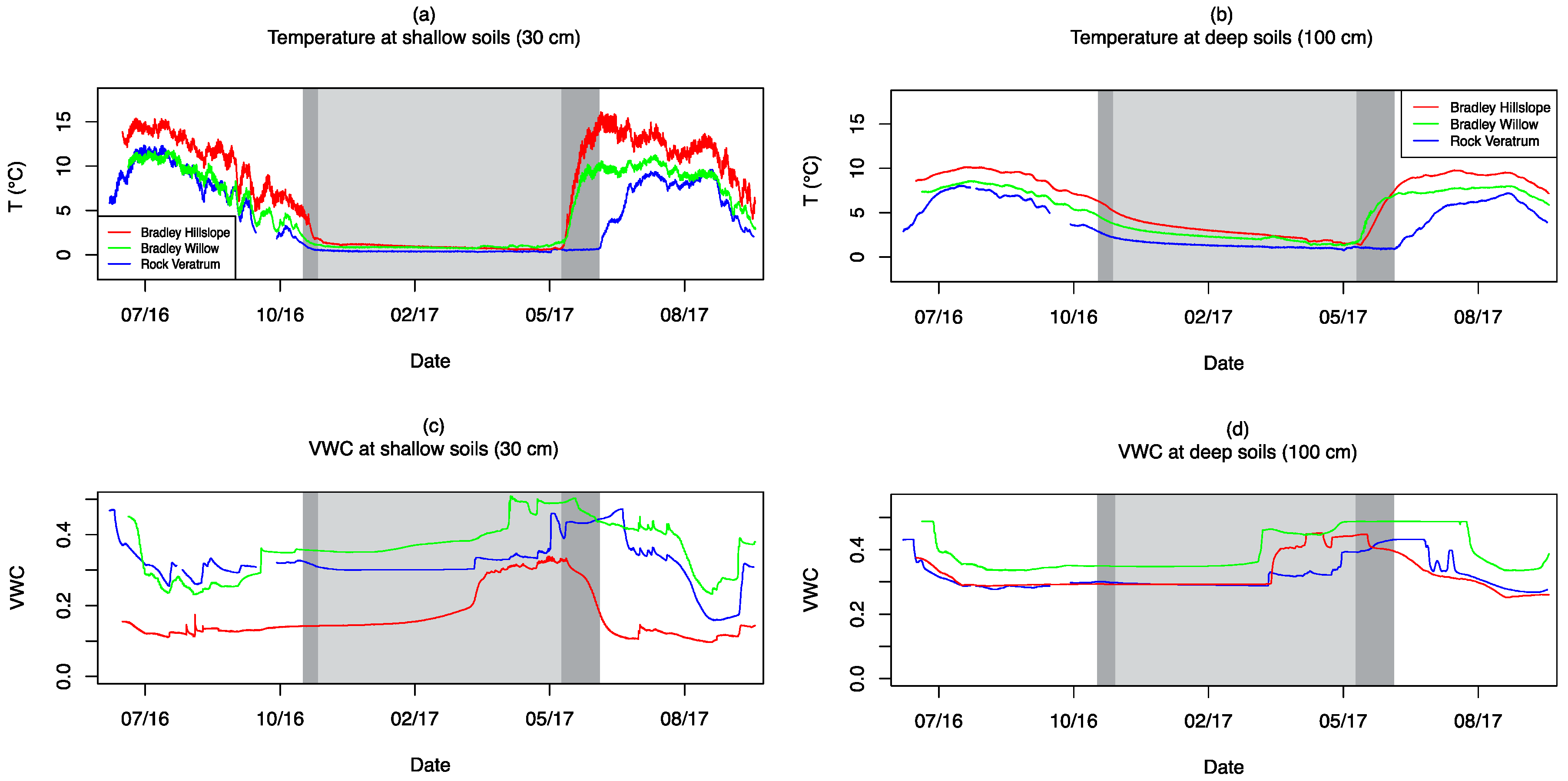
3.4. Soil Moisture and Temperature

Soil temperature and volumetric water content (VWC) across BCM, BCW, and RCM are shown for shallow (30 cm) and deep (100 cm) soil conditions in Figure 4 for the period from 1 July 2016 through 12 October 2017. As shown in Table 2, average soil temperatures are the highest at BCM and the lowest at RCM. Despite similar growing season values between BCW and RCM, annual average conditions are cooler for RCM due to a shorter growing season duration. At all sites, shallow temperatures are relatively stable at 0.3–1 °C during the winter months under snowpack as indicated by grey shades in Figure 4. Shallow temperatures begin to rise and display diurnal variability with the melting of snowpack in late May 2017 for BCM and BCW and late June 2017 for RCM (Figure 4a). The transition back to snowpack conditions occurs in mid-November 2016 for RCW (dark grey shades in Figure 4) and late November 2016 for BCM and BCW (light grey shades in Figure 4) based on decreases in diurnal variability. Taken together, BCM and BCW experiences roughly 190 days of snowpack-free conditions, whereas RCM experiences roughly 145 days of snowpack-free conditions, as indicated in the areas not covered in grey shades in Figure 4. Compared with the shallow soils, deep soil temperatures at all sites display colder growing season and warmer winter season conditions and reduced annual and no diurnal variability (Figure 4b).

Although direct comparisons of VWC measurements between sites are complicated by variability in porosity and soil clay content, general trends are used to qualitatively compare moisture conditions between the sites. At all sites, moisture in shallow soils increases during the late spring with melting snow and decreases in the mid/late summer. Pulse-type wetting events occur during the summer monsoon in August and September, and relatively stable conditions persist through winter under the snowpack, as indicated by the grey shades in Figure 4. As shown in Figure 4c, BCM experiences the driest conditions and an earlier dry-down period in early summer 2017, whereas BCW and RCM display similar water content and timing of annual trends. Deep soils display reduced variability in VWC, with relatively stable conditions through the late summer through winter and wetting up/drying down in the late spring/early summer (Figure 4d). In general, deep soils experience wetter average conditions than shallow soils at each site. Due to technical issues, continuous probe data are not available from RCF; however, soil conditions remain at or near saturation at the surface throughout the year based on field observations.

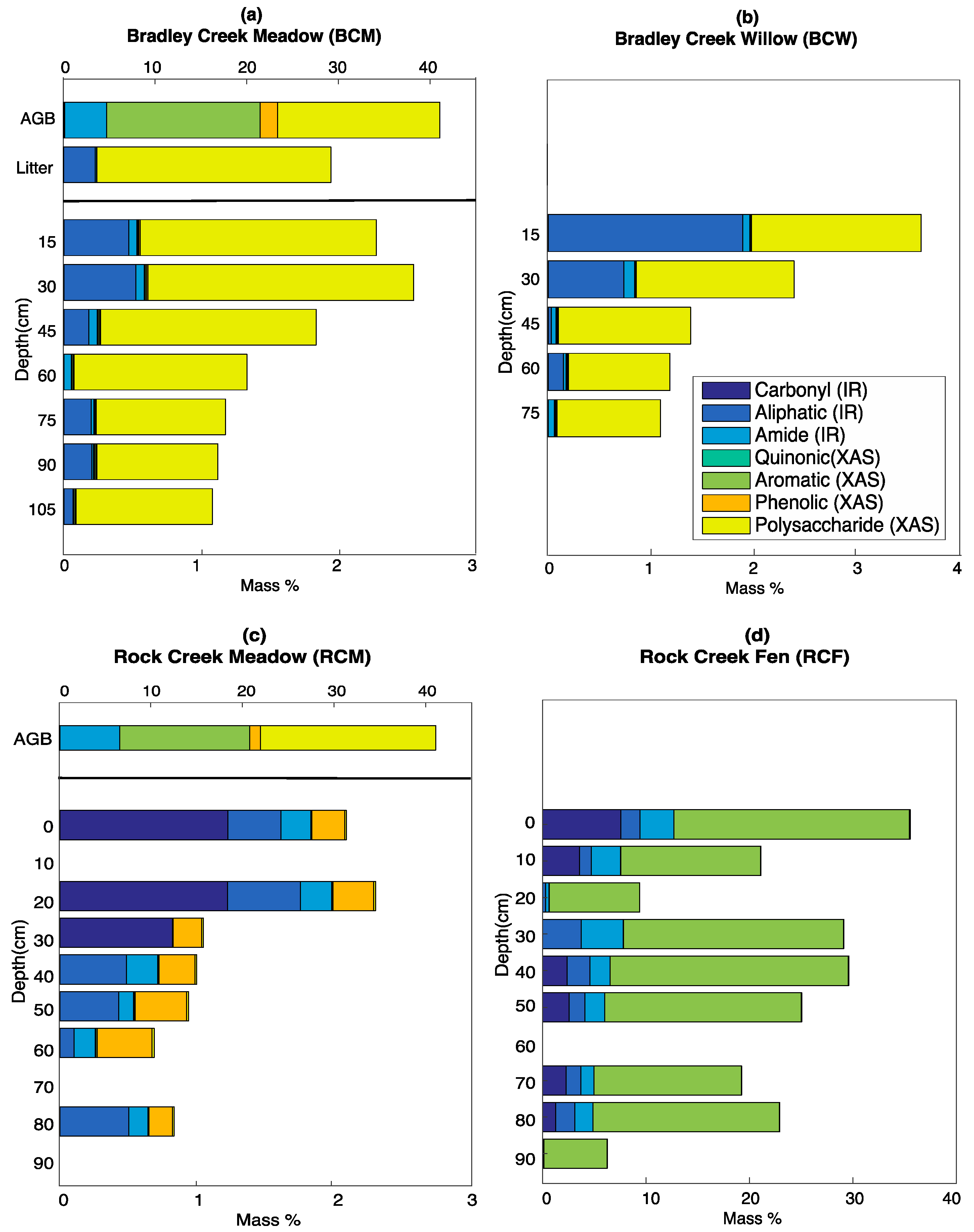
3.5. Calculated SOC Compositions

Organic carbon compositions of soils, above-ground biomass (AGB), and litter were calculated using the SOC-fga method (Figure 5) (see Supplementary Materials Figures S18–S22 for AGB FT-IR and XAS spectra, and Tables S9–S13 and Figure S23 for α_i values and linear mass balance fit results). In the absence of standard reference material, we performed a series of modeling tests to different approaches for implementing the SOC-fga method. Assuming seven functional groups, the peak areas corresponding to the functional groups for a minimum of seven related samples are required for Equation (8) to ensure a unique solution for α_i. First, in order to determine which sets of related samples to group in Equation (8), we tested three sample selection approaches for the SOC-fga method: (1) a universal fit, where all soil samples from BCM, BCW, RCM, and RCF are fit by Equation (8); (2) a site-specific fit, where soil samples collected from the same site across various depths were fit; and (3) a depth-specific fit, where soil samples with similar depths but from different sites were grouped (please see Supplementary Materials Section S3, Figures S5–S7, and Tables S1 and S2 for additional details). We concluded that a site-specific fit yields the most reliable results because the R² values between the experimental TOC and optimized TOC obtained by the site-specific fit are the highest, and slope t-tests showed that the differences between experimental TOC and optimized TOC is insignificant. In addition, XRF and PXRD experiments showed that major element compositions (Figures S8–S11, Table S3) and mineral phases (Figure S12) are more consistent within the same site than within the same depth range between different sites, which supports our conclusion that samples from the same site are more similar and should be grouped for Equation (8) (i.e., a site-specific fit). We also found that samples from BCM and BCW have very similar α_i values, possibly due to the spatial proximity between the two sites. Therefore, in this work, we grouped samples into three matrix equations: (1) BCM and BCW, (2) RCM, and (3) RCF (please see Supplementary Materials Section S2 for more details on the three fitting approaches).

Further, we also tested four boundary conditions for Equation (8) to account for the detection limits of FT-IR and bulk C XAS (please see Supplementary Materials Section S5, Figure S15, and Tables S6–S8 for more details on the boundary condition tests). We concluded that the boundary condition of α_i > 0.01 yields the best fitting results while ensuring that the calculated mass% for each functional group is above the detection limits of the instrument that measured it. Therefore, we calculated SOC compositions using site-specific fits with the boundary condition α_i > 0.01. BCM and BCW show similar SOC compositions with large proportions of polysaccharides and aliphatic compounds, and small amounts of quinonic, aromatic, and phenolic carbon. Although a substantial amount of aliphatic carbon is also present at RCM and RCF, the amount of polysaccharides is negligible. There is a substantial portion of carbonyl at the top 30 cm at RCM and at most depths at RCF. Further, more phenolic and aromatic carbon is present at RCM and RCF, respectively.

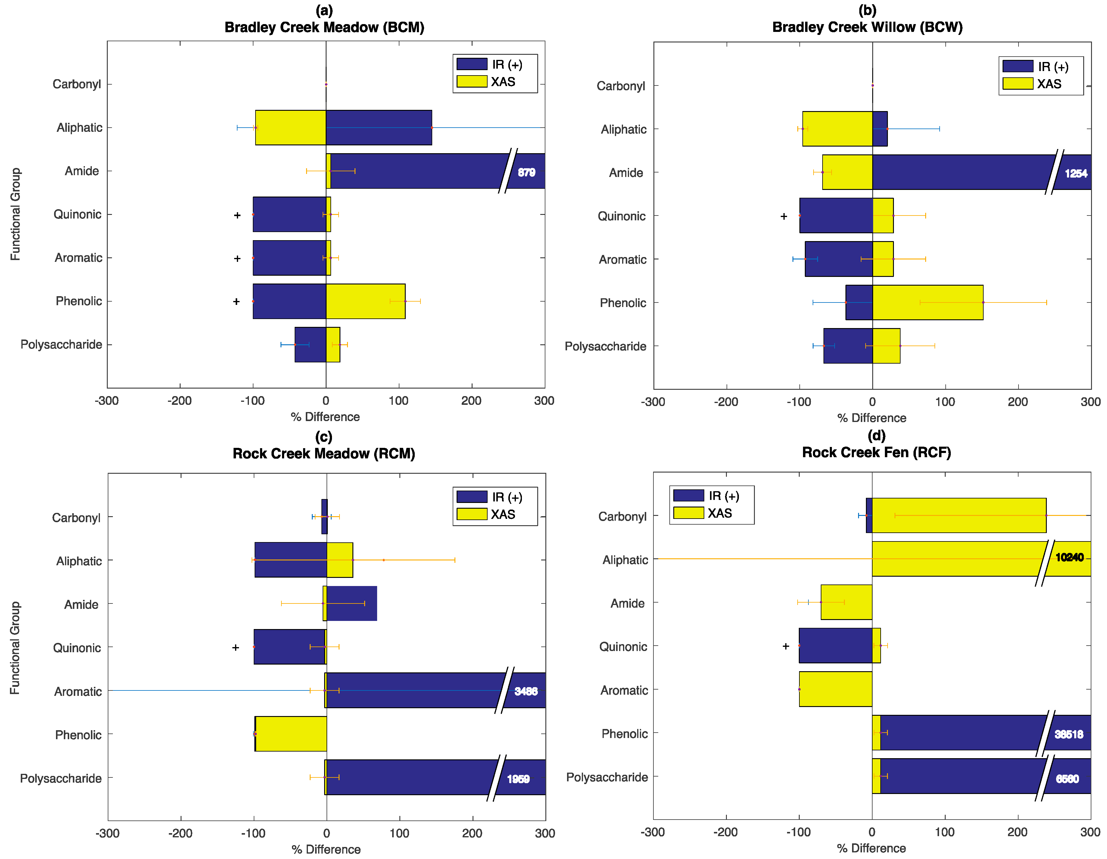
3.6. Evaluation of the SOC-fga Method Relative to Single Techniques

To evaluate the SOC-fga method, we compared the agreements between measured TOC and the optimized sum of organic carbon functional groups from Equation (8) using peak areas from individual techniques as well as the combined FT-IR/XAS SOC-fga method. The R² values between the experimental TOC measured by EA and optimized TOC using Equation (8) for each spectroscopic technique and the SOC-fga method at Bradley Creek (BC, which includes BCM and BCW), RCM, and RCF are listed in

Table 5. R² values between experimental TOC and optimized TOC for linear mass balance fits using FT-IR only, bulk C XAS only, and the SOC-fga method (both FT-IR and bulk C XAS are used), at BC, RCM, and RCF.

R2	BC	RCM	RCF	Average
FT-IR	0.8127	0.8549	0.9302	0.8659
XAS	0.6147	0.9181	0.9672	0.8335
SOC-fga (FT-IR/XAS)	0.9305	0.9203	0.9731	0.9413

. Because the experimentally measured TOC is used as the optimization criteria, the R² values represent how well the optimized TOC correlates with the experimentally measured TOC. The R² values are on average 8% to 11% higher for fits using the SOC-fga method that include peaks from both FT-IR and bulk C XAS compared to using either one of the spectroscopic techniques alone. This suggests that using both techniques to identify the functional groups that they are the most sensitive to results in improved solutions for α_i using Equation (8).

The R² values indicate that Equation (8) can be optimized with a set of α_i values using all three approaches (FT-IR, XAS, and SOC-fga), with the SOC-fga method yielding the highest R² values. To further understand the physical implications of the different fits, we compared the functional group abundance calculated by Equation (8) using the SOC-fga method versus individual spectroscopic techniques. Using results from Figure 5 as a reference, Figure 6 shows the average % difference for FT-IR and bulk C XAS for each functional group relative to the SOC-fga results (Equation (9)). In Figure 6, each bar shows the average % difference across all depth at each site for each functional group. The bars marked with “+” represent functional groups that are not observed (i.e., peak area = 0) by FT-IR at all depths at the given site.

At BC, the % difference is positive for the functional groups to which each technique is the most sensitive (average = +383.1% for FT-IR and +48.3% for bulk C XAS), especially amide for FT-IR and phenolic for bulk C XAS, and negative for functional groups to which a particular technique is not as sensitive (average = −79.9% for FT-IR and −42.5 for bulk C XAS) (Figure 6a,b). The smaller % difference for bulk C XAS suggests that it yields results that are more consistent with the SOC-fga method possibly because it represents a greater fraction (four) of the functional groups considered. Further, the results in Figure 6a,b suggest that if only one technique is used for Equation (8), the mass% of functional groups to which it is the most sensitive will be biased towards larger values. For example, if only FT-IR is used for Equation (8), the α_i values for the functional groups to which FT-IR is the most sensitive (i.e., carbonyl, aliphatic, and amide, as summarized in Table 1) are amplified by the algorithm, leading to a larger calculated mass% for these functional groups. By contrast, the α_i values for the functional groups to which FT-IR is not as sensitive (i.e., quinonic, aromatic, phenolic, and polysaccharide) are reduced by the algorithm, resulting in the calculated mass% of these functional groups being less. For example, the mass% of quinonic C at both BCM and BCW and the mass% of aromatic and phenolic C at BCM are zero because FT-IR did not identify these functional groups, even though peaks were detected by bulk C XAS. This is attributed to two factors: (1) FT-IR did not identify certain functional groups at all (i.e., peak area = 0), which means that only the peak areas for the functional groups that are identified (i.e., peak area > 0) can be used for Equation (8), leading to an amplification of α_i values for the functional groups that are identified; and (2) there are larger errors in peak area assignments for functional groups to which each technique is not the most sensitive, so in order to optimize the fit for Equation (8), the algorithm reduces the α_i values for said functional groups to minimize errors. The fact that these biases are consistent with instrumental sensitivities at the BC sites suggests that using both FT-IR and bulk C XAS as complementary approaches will provide a more holistic picture of SOC composition.

At RCM and RCF, the patterns for FT-IR and bulk C XAS are not as straightforward, and overall the standard deviations of the percent difference across all depth, as indicated by the error bars in Figure 6c,d, are larger than those at BC (for FT-IR, the average standard deviation of percent difference for all functional groups is 85.0 at BC, 838.2 at RCM, and 8136.6 at RCF; for bulk C XAS, the average standard deviation of percent difference for all functional groups is 23.6 at BC, 39.1 at RCM, and 385.9 at RCF). Because each technique detects a functional group (i.e., peak area > 0) at some depths but not the others (i.e., peak area = 0), this results in a different fit and a larger range of percent difference when compared to the mass% calculated from the SOC-fga method. For example, at RCM, while FT-IR identifies aromatic C at most depths, the peak area for aromatic C at 30 cm and 80 cm is zero, leading to a larger percent difference and hence a larger standard deviation. At RCF, the percent differences for both techniques are 10- to 80-fold larger than for the other three sites, especially for carbonyl, aliphatic, phenolic, and polysaccharide. Further, the average standard deviation of percent difference for all functional groups at RCF is about 10-fold larger than the other three sites for both techniques. Because RCF is a depositional fen and the soil matrix composition across depth is not as consistent compared to the other three sites, there may in reality be a larger variation in α_i values for each functional group across depth, although α_i is assumed to be constant for each functional group at each site in Equation (8). This deviation from our assumption that α_i is constant is likely to contribute to the larger percent difference and standard deviation at RCF. Therefore, the SOC-fga method will result in more consistent patterns when it is used at a site where the soil matrix and SOC composition (i.e., peak areas for functional groups are greater than zero at all depths) are similar across the samples used in the linear mass balance model.

To statistically compare the calculated SOC mass% between the SOC-fga method and individual techniques, we performed a pooled error variance t-test (p < 0.05) on all functional groups between (1) FT-IR and bulk C XAS, (2) the SOC-fga method versus FT-IR, and (3) the SOC-fga method versus bulk C XAS (please see Supplementary Materials Table S14–S16 for more details on the pooled error variance t-tests). The t-test results show that the differences in the calculated mass% for all functional groups between FT-IR and bulk C XAS are significant (p < 0.05) except for aromatic C. This suggests that if only FT-IR or bulk C XAS is used to quantify SOC composition with Equation (8), the results will not be consistent between the two techniques. Between FT-IR and the SOC-fga method, the differences in the calculated mass% are insignificant (p > 0.05) for quinonic C. Between bulk C XAS and the SOC-fga method, the differences in the calculated mass% are insignificant (p > 0.05) for aliphatic, quinonic, phenolic C, and polysaccharide. The differences are significant (p < 0.05) for all the other functional groups. In addition, the p-values for t-tests performed between FT-IR and bulk C XAS are larger than p-values between the SOC-fga method and either one of the techniques. The results from the t-tests suggest that, although there are statistical differences between the application of the SOC-fga method and a single technique, the SOC-fga method reconciles the discrepancies between FT-IR and bulk C XAS because the differences in calculated mass% between the SOC-fga method and FT-IR or bulk C XAS are statistically less significant compared to the differences in calculated mass% between FT-IR and bulk C XAS. The better agreement between the SOC-fga method and bulk C XAS (i.e., there are more functional groups with statistically insignificantly different calculated mass% between these two methods), combined with the lower percent difference and lower standard deviations of bulk C XAS, suggests that when only one analytical technique is available, bulk C XAS will produce SOC compositions that are more consistent with the SOC-fga method (see Section 4.4. for a more detailed discussion of limitations and future work).

The differences between SOC compositions calculated using only one spectroscopic technique and the SOC-fga method combining both FT-IR and bulk C XAS are not surprising given that different spectroscopic techniques have different sensitivities for different functional groups. In the absence of a peak for a particular functional group, such as quinonic C for FT-IR, the experimentally measured TOC is only assigned to functional groups that are detected, which alters the α_i values calculated by Equation (8). Examination of the resulting α_i values also indicates that the algorithm tends to amplify α_i values for functional groups to which a spectroscopic technique is the most sensitive while reducing α_i values for other functional groups to optimize the fit for Equation (8). In conclusion, by accounting for a broader range of functional groups in the application of the mass balance model, the combined FT-IR/XAS approach appears to present a more balanced quantification of the SOC composition. Regardless of which technique was used, the relative pattern of SOC composition at BC is consistent, with a substantial amount of polysaccharide and aliphatic and little quinonic, aromatic, and phenolic C. At RCM and RCF, an increased amount of polysaccharide C is calculated when only FT-IR is used. In addition, an increased amount of aliphatic C is calculated at RCF when only bulk C XAS is used. Nevertheless, carbonyl, aromatic, and phenolic C are still the major components at RC, indicating that the relative differences between the sites still exist regardless of which technique is used. In the future, to further enhance our understanding of how to optimally apply each spectroscopic technique, the results should be compared to other approaches, such as ¹³C NMR, and a set of standard reference materials developed and acknowledged by the SOC research community.

4. Discussion

Currently, inferences about the controls on SOC turnover are often based on carbon flux estimates combined with the partitioning of carbon into operationally defined fractions or “pools” [7]. Although knowledge of the underlying SOC composition is widely recognized to be an additional control on the mechanisms of SOC turnover and stabilization [2], this information is often not available due to the difficulties in quantifying SOC composition. Our SOC-fga method provides an approach to quantitatively study SOC composition while avoiding the complications resulting from harsh chemical treatments. Further, our results suggest that SOC compositions can be similar across two closely related sites with different landscape positions, and vastly different between sites with similar parent material and vegetation types but slightly different temperature and hydrologic conditions (Figure 5). Thus, expanding available methods of SOC characterization is a critical step towards a predictive understanding of subsurface carbon transformation.

The SOC-fga method combines the strengths of two spectroscopic techniques to quantitatively identify SOC functional groups. Examination of the individual spectra confirms the relative differences between the sites shown in Figure 5. For example, in FT-IR spectra (Figure 2), the peaks corresponding to carbonyl and amides are more dominant in RCM and RCF than in BC, which is consistent with the calculated results in Figure 5. Similarly, in the bulk C XAS spectra (Figure 3), polysaccharide has better-defined peak shapes and peak areas at BC comparing to RCM and RCF. The bulk C XAS spectra of RCF also show larger aromatic peaks. In addition, we have shown that the fits from Equation (8) improve when both FT-IR and XAS are used to identify the peaks for which they are optimized comparing to using either technique alone (Table 4). We have also demonstrated that although Equation (8) can quantify the SOC functional group abundances in all three cases, the resulting functional group mass% might be biased depending on which technique is used (Figure 6). Regardless of the technique(s) used, we found considerable differences between soils with similar landscape positions/vegetation types at two different elevations.

The similarities or differences in SOC composition between soils from different elevations and/or vegetation types inform our understanding of processes controlling the accumulation and transformation of SOC. There is notable similarity in SOC compositions between the BCM and BCW sampling locations (Figure 5a,b) each from the lower-elevation sampling area. In contrast, the SOC compositions at RCM and RCF differ significantly from the SOC composition at BC and from each other (Figure 5c,d). At RCM and RCF, polysaccharides are negligible while carbonyl and aliphatic compounds are abundant (Figure 5c,d). Further, phenolic and aromatic compounds make up substantial portions of the SOC at RCM and RCF, respectively. In the following section, we use the SOC functional group abundances calculated by the SOC-fga method to discuss the possible implications for factors controlling SOC speciation and transformations.

4.1. Inputs from Above-Ground Vegetation

Above-ground vegetation inputs can affect vertical SOC distribution [35,36,37,38]. For example, Guo et al. [37] reported that there is significantly more alkyl (aliphatic) C and less aryl (aromatic) C in planted mixed broad-leaved and coniferous forests compared to native broad-leaved forests and tea gardens in China, and that alkyl (aliphatic) C and aryl (aromatic) C are more sensitive to vegetation changes than other functional groups. Although the vegetation types and climate described in Guo et al.’s work are very different from ours, the aromatic C content is substantially different between BC, RCM, and RCB (Figure 5). This could be caused by different vegetation inputs if aromatic C is sensitive to vegetation differences. Furthermore, even though the chemical composition of AGB is similar between BCM and RCM (Figure 5a,c), there are differences in vegetation type and productivity between these two sites (Table 2). Compared to BCM, which is generally drier and has a longer growing season, RCM is completely covered by perennial forbs and has almost 2.5 times more AGB per unit area. The difference in productivity may result in different input rates and compositions of SOC.

We did not measure the chemical compositions of AGB at BCW and RCF due to the heterogeneity of the willows. The chemical composition at BCW is similar to that of BCM (Figure 5a,b). This may reflect the proximity of these two soil profiles: BCW is located downgradient of BCM and may thus receive similar plant litter inputs and/or input of mineral-associated SOC from BCM. Further, the graminoids and perennial forbs underneath the willows may be the major vegetation inputs at BCW. At RCF, because the willows have more structural materials and presumably a different allocation of above- and below-ground resources compared to meadow vegetation, vegetation input combined with prolonged exposure to groundwater presumably lead to the different SOC inputs.

Finally, all of the study sites are grazed by cattle at the end of the growing season. Both the consumption (removal) of plant materials and the input of cattle excrement may further influence the composition of SOC entering the soil at these sites [39,40,41]. For example, Wang et al. [40] reported that the content of aromatic C increased while O-alkyl C (polysaccharide) decreased after 4 years of grazing exclusion in inner Mongolian grasslands. Although we did not quantify cattle grazing pressure, BC is consistently under higher grazing pressure than RCM and RCF based on our field observations. The lower grazing pressure at RCM and RCF may lead to higher aromatic content and lower O-alkyl content, as suggested by Wang et al. [40], and a more thorough study of grazing activities over a longer period of time is necessary to confirm the relationship between grazing and SOC composition at our sites. The difference in the ease of access of these sites by cattle and the timing of grazing due to elevation have the potential to further influence site level differences in the above-ground SOC that enters the soils.

4.2. Internal Processing and Losses

Given that soil microbes are an important control on SOC turnover and accumulation [9,42,43], the differences in microbial-driven processing and SOC losses between different sites can lead to different SOC compositions. At BCM, although there is a significant amount of aromatic and quinonic carbon in above-ground biomass, the abundance of these compounds in soil samples is negligible. Further, litter at BCM contains very little aromatic carbon, suggesting that although aromatic compounds are often considered recalcitrant [11,44,45], plant-derived aromatic carbon in litter is quickly decomposed at the soil surface [46]. On the other hand, polysaccharides, which can in theory be readily decomposed, are present in substantial quantities. Compared with above-ground biomass, the portion of polysaccharides is larger in litter and soil, which could be caused by preferential loss of aromatics or other sources of polysaccharides in soil, such as inputs from microbial reprocessing or below-ground plant inputs [47]. For example, plant root mucilage and extracellular polymeric substances (EPS), which are drought defense mechanisms for plants and soil microbes, respectively [48,49], are mostly polysaccharide [50,51,52] and could contribute to the high polysaccharide content at the drier BCM site.

The lack of aromatic, quinonic, and phenolic compounds at BC directly contrasts with the predictions based on chemical recalcitrance, as these compounds are more thermodynamically stable and hence should be more resistant to microbial decomposition [11,44,45]. Recently, studies have shown that chemical recalcitrance is not the only, and in some cases even not the primary, factor that determines SOC turnover and stabilization, and hence thermodynamically stable aromatic compounds are not necessarily the most dominant organic species in soil [2,6,42,53,54,55]. For example, humics from the Georgetown Wetlands in North Carolina were shown to contain greater abundances of polysaccharide versus aromatic SOC [56]. Furthermore, SOC with long turnover times has been shown to be compositionally distinct from plant materials [57]. More recently, Kallenbach et al. [47] demonstrated that SOC accumulation and composition can be strongly influenced by microbial communities in soil, and that compounds previously thought to be chemically recalcitrant make up a relatively small fraction of SOC (~5–15%), while polysaccharide-like molecules can make up ~30% of SOC. In light of these recent findings, our results suggest that site level difference in the processes controlling the internal cycling of SOC is an important driver of the SOC composition across our study area.

4.3. Environmental Factors

Environmental factors, such as soil temperature, moisture, and seasonality, are known to influence microbially mediated SOC composition [58,59,60,61,62]. BCM and BCW are warmer for a longer period of time throughout the year compared to RCM (Figure 4a,b). The higher average temperatures at BC should offset the lower plant productivity and result in increased degradation of compounds previously considered to be recalcitrant (quinonic, aromatic, and phenolic compounds). In contrast, lower average temperatures at RCM can result in slower microbial decomposition, leading to a larger amount of incompletely oxidized carbonyl and phenolic compounds [63,64].

Transient oxygen-limitation due to prolonged wet conditions may also play an important role between the sites. RCM has lower average temperatures and a growing season that is about 45 days shorter than BC due to prolonged snow cover (Figure 4). This may result in longer periods of dormancy or reduced microbial activity in soils at RCM throughout the year, leading to slower SOC decomposition. RCF is perennially saturated based on field observations, and because the TOC at RCF is an order of magnitude higher than at the other three sites, we conclude that limitation on oxygen levels at RCF is a dominant driver of SOC composition, and we cannot rule out oxygen-limited conditions at RCM for at least part of the year based on the observed SOC composition in Figure 5. Extracellular phenol oxidase and peroxidase are a central control on microbial lignin decomposition, and thus oxygen limitations at RCF, and likely at RCM, due to saturated conditions could lead to a slower decomposition of complex aromatic structures and hence an accumulation of aromatics [65,66]. Further, polycyclic aromatic compounds are known to form and accumulate in soils under oxygen-deficient conditions [67,68], supporting our observations at RCM and RCF. In addition, at RCF, with even higher soil moisture and lower oxygen content than RCM, oxidation of aromatic compounds into phenolic compounds may be retarded, resulting in accumulation of aromatic compounds at RCF, which is consistent with previous studies of peat formation [69,70]. Future work will interrogate the microbial communities, redox systematics, and the timing and duration of snowmelt to enhance our understanding of how soil microbes affect SOC composition.

In summary, although our observations of SOC composition and variations between field sites at different elevation are broadly consistent with the diverse results from experimental and field-based studies of SOC, further investigation into soil microbial activities and physical protection of SOC will be required to confirm the drivers behind the large differences in functional groups.

4.4. Limitations of and Outlooks for the SOC-fga Method

Although our collective results suggest that the SOC-fga method combining FT-IR and bulk C XAS is a promising new approach for quantifying SOC composition, the method will need to be combined with additional studies of carbon turnover, microbial communities, and respiration rates in order to fully evaluate how differences in ecosystem and environmental drivers affect SOC storage and decomposition. Although the qualitative comparison among spectra across the sites supports our quantitative SOC-fga model, we cannot yet assess the external errors associated with our calculations due to the lack of reference soils with a well-characterized SOC composition. As additional methods that provide quantitative assessment of SOC composition become available, it will be essential to establish adequate soil reference materials for method validation and laboratory inter-comparisons. With the establishment of reference materials, accurately benchmarking the SOC-fga method against existing characterization techniques, such as MS or NMR, will be feasible, although both techniques introduce their own complications for quantifying SOC composition. All analytical methods are likely to have their own biases, and knowledge of these biases will support data interpretation, comparison among sites, and ultimately the development of more robust models.

In addition, we have shown that the SOC-fga method results in more consistent patterns when the linear mass balance fit is applied to soil samples whose matrix and SOC composition are more consistent. In our work, we achieved this consistency by using a minimum of seven (i.e., the number of functional groups identified) soil samples from the same profile. Although we are confident that the SOC-fga method can be applied to soil samples in other ecosystems, the α_i values in our study cannot be directly used for other soils. Applying this method to soils from different ecosystems and formed from different parent materials will allow further assessment of the limitations of the SOC-fga method, as well as an improved quantitative understanding of the variations between different soils.

5. Conclusions

In conclusion, we have demonstrated that the SOC-fga method, a novel approach that combines the strengths of FT-IR and bulk C XAS, can quantify SOC functional groups while avoiding complications caused by chemical treatments. This method will allow us to incorporate quantitative and measurable parameters (i.e., the abundance of various SOC functional groups) into earth system models to help us interrogate the mechanisms and rates of SOC turnover and stabilization, and the feedbacks between SOC and climate change. Although considerably more time-intensive, the SOC-fga method provides a useful and more quantitative alternative to characterization than using FT-IR or bulk C XAS alone. To further improve the accuracy of this method, it is important to validate it against standard soil samples with known SOC composition, other analytical techniques, and further assess it with soil samples from a variety of ecosystems. Nevertheless, meaningful quantification of SOC functional group abundances across biological and environmental gradients will greatly enhance our ability to resolve the underlying controls on SOC turnover and stabilization. This approach provides a much-needed bridge between estimates of SOC composition and increasingly mechanistic models of SOC cycling [71]. Finally, additional studies, such as density fractionation to investigate SOC physical protection, radiocarbon dating, and microbial profiling can be coupled with the SOC-fga method to further study SOC turnover mechanisms.

References

1. Scharlemann, J.P.; Tanner, E.V.; Hiederer, R.; Kapos, V. Global soil carbon: Understanding and managing the largest terrestrial carbon pool. Carbon Manag. 2014. [Google Scholar] [CrossRef]
2. Schmidt, M.W.I.; Torn, M.S.; Abiven, S.; Dittmar, T.; Guggenberger, G.; Janssens, I.A.; Kleber, M.; Kögel-Knabner, I.; Lehmann, J.; Manning, D.A.C.; et al. Persistence of soil organic matter as an ecosystem property. Nature 2011, 478, 49–56. [Google Scholar] [CrossRef] [PubMed]
3. Gregory, J.M.; Jones, C.D.; Cadule, P.; Friedlingstein, P. Quantifying Carbon Cycle Feedbacks. J. Clim. 2009, 22, 5232–5250. [Google Scholar] [CrossRef]
4. Piao, S.; Sitch, S.; Ciais, P.; Friedlingstein, P.; Peylin, P.; Wang, X.; Ahlström, A.; Anav, A.; Canadell, J.G.; Cong, N.; et al. Evaluation of terrestrial carbon cycle models for their response to climate variability and to CO2 trends. Glob. Chang. Biol. 2013, 19, 2117–2132. [Google Scholar] [CrossRef] [PubMed]
5. Kleber, M.; Eusterhues, K.; Keiluweit, M.; Mikutta, C.; Mikutta, R.; Nico, P.S. Mineral-Organic Associations: Formation, Properties, and Relevance in Soil Environments. In Advances in Agronomy; Elsevier: San Diego, CA, USA, 2015; Volume 130, pp. 1–140. ISBN 9780128021378. [Google Scholar]
6. Kleber, M.; Nico, P.S.; Plante, A.; Filley, T.; Kramer, M.; Swanston, C.; Sollins, P. Old and stable soil organic matter is not necessarily chemically recalcitrant: Implications for modeling concepts and temperature sensitivity. Glob. Chang. Biol. 2011, 17, 1097–1107. [Google Scholar] [CrossRef]
7. Lehmann, J.; Kleber, M. The contentious nature of soil organic matter. Nature 2015, 528, 60–68. [Google Scholar] [CrossRef] [PubMed]
8. Xu, J.-M.; Huang, P.M. Molecular Environmental Soil Science at the Interfaces in the Earth’s Critical Zone; Springer Science & Business Media: New York, NY, USA, 2011; ISBN 9783642052972. [Google Scholar]
9. Schimel, J.P.; Schaeffer, S.M. Microbial control over carbon cycling in soil. Front. Microbiol. 2012, 3, 348. [Google Scholar] [CrossRef] [PubMed]
10. Don, A.; Böhme, I.H.; Dohrmann, A.B.; Poeplau, C.; Tebbe, C.C. Microbial community composition affects soil organic carbon turnover in mineral soils. Biol. Fertil. Soils 2017, 53, 445–456. [Google Scholar] [CrossRef]
11. Kleber, M.; Johnson, M.G. Advances in Understanding the Molecular Structure of Soil Organic Matter, 1st ed.; Elsevier Inc.: San Diego, CA, USA, 2010; Volume 106, ISBN 9780123810359. [Google Scholar]
12. Ikeya, K.; Sleighter, R.L.; Hatcher, P.G.; Watanabe, A. Fourier transform ion cyclotron resonance mass spectrometric analysis of the green fraction of soil humic acids. Rapid Commun. Mass Spectrom. 2013, 27, 2559–2568. [Google Scholar] [CrossRef] [PubMed]
13. Grandy, A.S.; Neff, J.C. Molecular C dynamics downstream: The biochemical decomposition sequence and its impact on soil organic matter structure and function. Sci. Total Environ. 2008, 404, 297–307. [Google Scholar] [CrossRef] [PubMed]
14. Baldock, J.A.; Oades, J.M.; Waters, A.G.; Peng, X.; Vassallo, A.M.; Wilson, M.A. Aspects of the chemical structure of soil organic materials as revealed by solid-state 13C NMR spectroscopy. Biogeochemistry 1992, 16, 1–42. [Google Scholar] [CrossRef]
15. Skjemstad, J.O.; Clarke, P.; Taylor, J.A.; Oades, J.M.; Newman, R.H. The removal of magnetic materials from surface soils. A solid state 13C CP/MAS NMR study. Aust. J. Soil Res. 1994, 32, 1215–1229. [Google Scholar] [CrossRef]
16. Schäfer, T.; Hertkorn, N.; Artinger, R.; Claret, F.; Bauer, A. Functional group analysis of natural organic colloids and clay association kinetics using C(1s) spectromicroscopy. J. Phys. IV 2003, 104, 409–412. [Google Scholar] [CrossRef]
17. Keeler, C.; Maciel, G.E. Quantitation in the Solid-State 13C NMR Analysis of Soil and Organic Soil Fractions. Anal. Chem. 2003, 75, 2421–2432. [Google Scholar] [CrossRef] [PubMed]
18. Mathers, N.J.; Xu, Z. Solid-state 13C NMR spectroscopy: Characterization of soil organic matter under two contrasting residue management regimes in a 2-year-old pine plantation of subtropical Australia. Geoderma 2003, 114, 19–31. [Google Scholar] [CrossRef]
19. Schmidt, M.W.I.; Knicker, H.; Hatcher, P.G.; Kogel-Knabner, I. Improvement of 13C and 15N CPMAS NMR spectra of bulk soils, particle size fractions and organic material by treatment with 10% hydrofluoric acid. Eur. J. Soil Sci. 1997, 48, 319–328. [Google Scholar] [CrossRef]
20. Sanderman, J.; Farrell, M.; Macreadie, P.I.; Hayes, M.; McGowan, J.; Baldock, J. Is demineralization with dilute hydrofluoric acid a viable method for isolating mineral stabilized soil organic matter? Geoderma 2017, 304, 4–11. [Google Scholar] [CrossRef]
21. Mathers, N.J.; Mao, X.A.; Saffigna, P.G.; Xu, Z.H.; Berners-Price, S.J.; Perera, M.C.S. Recent advances in the application of 13C and 15N NMR spectroscopy to soil organic matter studies. Soil Res. 2000, 38, 769–787. [Google Scholar] [CrossRef]
22. Gillespie, A.W.; Phillips, C.L.; Dynes, J.J.; Chevrier, D.; Regier, T.Z.; Peak, D. Advances in Using Soft X-Ray Spectroscopy for Measurement of Soil Biogeochemical Processes; Elsevier: San Diego, CA, USA, 2015; Volume 133, pp. 1–32. ISBN 9780128030523. [Google Scholar]
23. Parikh, S.; Goyne, K.; Margenot, A.; Mukome, F.; Calderón, F. Soil Chemical Insights Provided through Vibrational Spectroscopy. In Advances in Agronomy; Elsevier: San Diego, CA, USA, 2014; Volume 126, pp. 1–148. ISBN 9780128021325. [Google Scholar]
24. Solomon, D.; Lehmann, J.; Kinyangi, J.; Liang, B.; Schafer, T. Carbon K-edge NEXAFS and FTIR-ATR spectroscopic investigation of organic carbon speciation in soils. Soil Sci. Soc. Am. J. 2005, 69, 107–119. [Google Scholar] [CrossRef]
25. Heymann, K.; Lehmann, J.; Solomon, D.; Schmidt, M.W.I.; Regier, T. C 1s K-edge near edge X-ray absorption fine structure (NEXAFS) spectroscopy for characterizing functional group chemistry of black carbon. Org. Geochem. 2011, 42, 1055–1064. [Google Scholar] [CrossRef]
26. Wan, J.; Tyliszczak, T.; Tokunaga, T.K. Organic carbon distribution, speciation, and elemental correlations within soil microaggregates: Applications of STXM and NEXAFS spectroscopy. Lawrence Berkeley Natl. Lab. 2007, 71, 5439–5449. [Google Scholar] [CrossRef]
27. Loeppert, R.H.H.; Suarez, D.L.L. Carbonate and Gympusm. In Methods of Soil Analysis. Part 3. Chemical Methods—SSSA; Soil Science Society of America and American Society of Agronomy: Madison, WI, USA, 1996; pp. 455–456. [Google Scholar]
28. Margenot, A.J.; Calderón, F.J.; Bowles, T.M.; Parikh, S.J.; Jackson, L.E. Soil Organic Matter Functional Group Composition in Relation to Organic Carbon, Nitrogen, and Phosphorus Fractions in Organically Managed Tomato Fields. Soil Sci. Soc. Am. J. 2015, 79, 772. [Google Scholar] [CrossRef]
29. Swinehart, D.F. The Beer-Lambert Law. J. Chem. Educ. 1962, 39, 333. [Google Scholar] [CrossRef]
30. Calloway, D. Beer-Lambert Law. J. Chem. Educ. 1997, 74, 744. [Google Scholar] [CrossRef]
31. Ricci, R.W.; Ditzler, M.; Nestor, L.P. Discovering the Beer-Lambert Law. J. Chem. Educ. 1994, 71, 983. [Google Scholar] [CrossRef]
32. Bartholomew, W.V.; Clark, F.E.; Stevenson, F.J. Origin and Distribution of Nitrogen in Soil; American Society of Agronomy: Madison, WI, USA, 1965; ISBN 9780891182054. [Google Scholar]
33. Bartholomew, W.V.; Clark, F.E.; Bremner, J.M. Organic Nitrogen in Soils. In Soil Nitrogen; American Society of Agronomy: Madison, WI, USA, 1965; Volume 10, pp. 93–149. [Google Scholar]
34. Schulten, H.-R.; Schnitzer, M. The chemistry of soil organic nitrogen: A review. Biol. Fertil. Soils 1997, 26, 1–15. [Google Scholar] [CrossRef]
35. Jobbágy, E.G.; Jackson, R.B. The Vertical Distribution of Soil Organic Carbon and its Relation to Climate and Vegetation. Ecol. Appl. 2000, 10, 423–436. [Google Scholar] [CrossRef]
36. Kuzyakov, Y.; Domanski, G. Carbon input by plants into the soil. Review. J. Plant Nutr. Soil Sci. 2000, 163, 421–431. [Google Scholar] [CrossRef]
37. Guo, X.; Meng, M.; Zhang, J.; Chen, H.Y.H. Vegetation change impacts on soil organic carbon chemical composition in subtropical forests. Sci. Rep. 2016, 6, 29607. [Google Scholar] [CrossRef] [PubMed]
38. Wang, H.; Liu, S.-R.; Wang, J.-X.; Shi, Z.-M.; Xu, J.; Hong, P.-Z.; Yu, H.-L.; Chen, L.; Lu, L.-H.; Cai, D.-X. Differential effects of conifer and broadleaf litter inputs on soil organic carbon chemical composition through altered soil microbial community composition, An-Gang Ming. Nat. Publ. Gr. 2016. [Google Scholar] [CrossRef] [PubMed]
39. Piñeiro, G.; Paruelo, J.M.; Oesterheld, M.; Jobbágy, E.G. Pathways of Grazing Effects on Soil Organic Carbon and Nitrogen. Rangel. Ecol. Manag. 2010, 63, 109–119. [Google Scholar] [CrossRef]
40. Wang, C.; He, N.; Zhang, J.; Lv, Y.; Wang, L. Long-Term Grazing Exclusion Improves the Composition and Stability of Soil Organic Matter in Inner Mongolian Grasslands. PLoS ONE 2015, 10, e0128837. [Google Scholar] [CrossRef] [PubMed]
41. Eldridge, D.J.; Poore, A.G.B.; Ruiz-Colmenero, M.; Letnic, M.; Soliveres, S. Ecosystem structure, function, and composition in rangelands are negatively affected by livestock grazing. Ecol. Appl. 2016, 26, 1273–1283. [Google Scholar] [CrossRef] [PubMed] [Green Version]
42. Allison, S.D.; Wallenstein, M.D.; Bradford, M.A. Soil-carbon response to warming dependent on microbial physiology. Nat. Geosci. 2010, 3, 336–340. [Google Scholar] [CrossRef]
43. Fontaine, S.; Barot, S. Size and functional diversity of microbe populations control plant persistence and long-term soil carbon accumulation. Ecol. Lett. 2005, 8, 1075–1087. [Google Scholar] [CrossRef]
44. Sollins, P.; Homann, P.; Caldwell, B.A. Stabilization and destabilization of soil organic matter: Mechanisms and controls. Geoderma 1996, 74, 65–105. [Google Scholar] [CrossRef]
45. Brady, N.C.; Weil, R.R. The Nature and Properties of Soils; Pearson Education Limited: London, UK, 2008; ISBN 9780135133873. [Google Scholar]
46. Cotrufo, M.F.; Soong, J.L.; Horton, A.J.; Campbell, E.E.; Haddix, M.L.; Wall, D.H.; Parton, W.J. Formation of soil organic matter via biochemical and physical pathways of litter mass loss. Nat. Geosci. 2015, 8, 776–779. [Google Scholar] [CrossRef]
47. Kallenbach, C.M.; Frey, S.D.; Grandy, A.S. Direct evidence for microbial-derived soil organic matter formation and its ecophysiological controls. Nat. Commun. 2016, 7, 13630. [Google Scholar] [CrossRef] [PubMed]
48. Brunner, I.; Herzog, C.; Dawes, M.A.; Arend, M.; Sperisen, C. How tree roots respond to drought. Front. Plant Sci. 2015, 6, 547. [Google Scholar] [CrossRef] [PubMed]
49. Or, D.; Smets, B.F.; Wraith, J.M.; Dechesne, A.; Friedman, S.P. Physical constraints affecting bacterial habitats and activity in unsaturated porous media—A review. Adv. Water Resour. 2007, 30, 1505–1527. [Google Scholar] [CrossRef]
50. Jiao, Y.; Cody, G.D.; Harding, A.K.; Wilmes, P.; Schrenk, M.; Wheeler, K.E.; Banfield, J.F.; Thelen, M.P. Characterization of extracellular polymeric substances from acidophilic microbial biofilms. Appl. Environ. Microbiol. 2010, 76, 2916–2922. [Google Scholar] [CrossRef] [PubMed]
51. Walker, T.S.; Grotewold, E.; Vivanco, J.M. Update on Root Exudation and Rhizosphere Biology Root Exudation and Rhizosphere Biology 1. Plant Physiol. 2003, 132. [Google Scholar] [CrossRef] [PubMed]
52. Baetz, U.; Martinoia, E. Root exudates: The hidden part of plant defense. Trends Plant Sci. 2014, 19, 90–98. [Google Scholar] [CrossRef] [PubMed] [Green Version]
53. Xu, X.; Luo, Y.; Zhou, J. Carbon quality and the temperature sensitivity of soil organic carbon decomposition in a tallgrass prairie. Soil Biol. Biochem. 2012, 50, 142–148. [Google Scholar] [CrossRef]
54. Dungait, J.A.J.; Hopkins, D.W.; Gregory, A.S.; Whitmore, A.P. Soil organic matter turnover is governed by accessibility not recalcitrance. Glob. Chang. Biol. 2012, 18, 1781–1796. [Google Scholar] [CrossRef]
55. Todd-Brown, K.E.O.; Randerson, J.T.; Post, W.M.; Hoffman, F.M.; Tarnocai, C.; Schuur, E.A.G.; Allison, S.D. Causes of variation in soil carbon simulations from CMIP5 Earth system models and comparison with observations. Biogeosciences 2013, 10. [Google Scholar] [CrossRef]
56. Baveye, P.; Pariange, J.-Y.; Stewart, B.A. Revival: Fractals in Soil Science (1998): Advances in Soil Science—Philippe Baveye, Jean-Yves Parlange, Bobby A. Stewart—Google Books; CRC Press: Boca Raton, FL, USA, 1998. [Google Scholar]
57. Miltner, A.; Bombach, P.; Schmidt-Brücken, B.; Kästner, M. SOM genesis: Microbial biomass as a significant source. Biogeochemistry 2012, 111, 41–55. [Google Scholar] [CrossRef]
58. Bryant, J.A.; Lamanna, C.; Morlon, H.; Kerkhoff, A.J.; Enquist, B.J.; Green, J.L. Colloquium paper: Microbes on mountainsides: Contrasting elevational patterns of bacterial and plant diversity. Proc. Natl. Acad. Sci. USA 2008, 105 (Suppl. 1), 11505–11511. [Google Scholar] [CrossRef] [PubMed]
59. Pietikäinen, J.; Pettersson, M.; Bååth, E. Comparison of temperature effects on soil respiration and bacterial and fungal growth rates. FEMS Microbiol. Ecol. 2005, 52, 49–58. [Google Scholar] [CrossRef] [PubMed]
60. Allison, S.D.; Treseder, K.K. Warming and drying suppress microbial activity and carbon cycling in boreal forest soils. Glob. Chang. Biol. 2008, 14, 2898–2909. [Google Scholar] [CrossRef]
61. Xiang, S.-R.; Doyle, A.; Holden, P.A.; Schimel, J.P. Drying and rewetting effects on C and N mineralization and microbial activity in surface and subsurface California grassland soils. Soil Biol. Biochem. 2008, 40, 2281–2289. [Google Scholar] [CrossRef]
62. Brockett, B.F.T.; Prescott, C.E.; Grayston, S.J. Soil moisture is the major factor influencing microbial community structure and enzyme activities across seven biogeoclimatic zones in western Canada. Soil Biol. Biochem. 2012, 44, 9–20. [Google Scholar] [CrossRef]
63. Zobell, C.E. Microbial Degradation of Oil: Present Status, Problems, and Perspectives. In The Microbial Degradation of Oil Pollutants; Louisiana State University: Baton Rouge, LA, USA, 1973; Volume 126, pp. 3–16. [Google Scholar]
64. Riser-Roberts, E. Remediation of Petroleum Contaminated Soils: Biological, Physical, and Chemical Processes; CRC Press: Boca Raton, FL, USA, 1998; ISBN 9781420050578. [Google Scholar]
65. Lindahl, B.D.; Tunlid, A. Ectomycorrhizal fungi—Potential organic matter decomposers, yet not saprotrophs. New Phytol. 2015, 205, 1443–1447. [Google Scholar] [CrossRef] [PubMed]
66. Sinsabaugh, R.L. Phenol oxidase, peroxidase and organic matter dynamics of soil. Soil Biol. Biochem. 2010, 42, 391–404. [Google Scholar] [CrossRef]
67. Thiele, S.; Brümmer, G.W. Bioformation of polycyclic aromatic hydrocarbons in soil under oxygen deficient conditions. Soil Biol. Biochem. 2002, 34, 733–735. [Google Scholar] [CrossRef]
68. Tsibart, A.S.; Gennadiev, A.N. Polycyclic aromatic hydrocarbons in soils: Sources, behavior, and indication significance (a review). Eurasian Soil Sci. 2013, 46, 728–741. [Google Scholar] [CrossRef]
69. Krull, E.S.; Thompso, C.H.; Skjemstad, J.O. Chemistry, radiocarbon ages, and development of a subtropical acid peat in Queensland, Australia. Aust. J. Soil Res. 2004, 42, 411–425. [Google Scholar] [CrossRef]
70. Freitas, J.C.C.; Bonagamba, T.J.; Emmerich, F.G. 13C High-Resolution Solid-State NMR Study of Peat Carbonization. Energy Fuels 1999, 13, 53–59. [Google Scholar] [CrossRef]
71. Li, L.; Maher, K.; Navarre-Sitchler, A.; Druhan, J.; Meile, C.; Lawrence, C.; Moore, J.; Perdrial, J.; Sullivan, P.; Thompson, A.; et al. Expanding the role of reactive transport models in critical zone processes. Earth Sci. Rev. 2017, 165, 280–301. [Google Scholar] [CrossRef]
Figure 1. Total nitrogen (TN) and total organic carbon (TOC) depth profiles at (a) BCM; (b) BCW; (c) RCM; and (d) RCF. Note the change of scale on panel (d) RCF. TC: total carbon.
Soilsystems 02 00006 g001
Figure 2. FT-IR depth profiles of (a) BCM; (b) BCW; (c) RCM; and (d) RCF. Vertical lines: peak centroids used for linear mass balance fit.
Soilsystems 02 00006 g002
Figure 3. Bulk C XAS depth profiles of (a) BCM; (b) BCW; (c) RCM; and (d) RCF. Vertical lines: peaks used for linear mass balance fit.
Soilsystems 02 00006 g003
Figure 4. Temperature at (a) shallow soils (30 cm) and (b) deep soils (100 cm), and volumetric water content (VWC) at (c) shallow soils (30 cm) and (d) deep soils (100 cm) at BCM (red), BCW (green), and RCM (blue). The light grey shades indicate the snow-covered periods at Bradley Creek (BC), and the dark grey shades indicate the additional snow-covered periods at RCM.
Soilsystems 02 00006 g004
Figure 5. Organic carbon composition at (a) BCM; (b) BCW; (c) RCM; and (d) RCF calculated using the SOC-fga method. Note the change of scale on panel RCF.
Soilsystems 02 00006 g005
Figure 6. The average percent difference in mass% between FT-IR and the SOC-fga method (blue) or between bulk X CAS and the SOC-fga (yellow) for all SOC functional groups at (a) BCM; (b) BCW; (c) RCM; and (d) RCF. The “+”signs represent functional groups that are not observed (i.e., peak area = 0) in FT-IR at all depth for the site.
Soilsystems 02 00006 g006