Implicit Temporal Discretization and Exact Energy Conservation for Particle Methods Applied to the Poisson–Boltzmann Equation

Abstract

We report on a new multiscale method approach for the study of systems with wide separation of short-range forces acting on short time scales and long-range forces acting on much slower scales. We consider the case of the Poisson–Boltzmann equation that describes the long-range forces using the Boltzmann formula (i.e., we assume the medium to be in quasi local thermal equilibrium). We develop a new approach where fields and particle information (mediated by the equations for their moments) are solved self-consistently. The new approach is implicit and numerically stable, providing exact energy conservation. We test different implementations that all lead to exact energy conservation. The new method requires the solution of a large set of non-linear equations. We consider three solution strategies: Jacobian Free Newton Krylov, an alternative, called field hiding which is based on hiding part of the residual calculation and replacing them with direct solutions and a Direct Newton Schwarz solver that considers a simplified, single, particle-based Jacobian. The field hiding strategy proves to be the most efficient approach.

1. Introduction

Matter in any form or state is characterized by the presence of particles interacting via fields. At the most fundamental level, a quantum point of view is needed, but as larger and larger portions of matter need to be studied, attention shifts from the quantum level to the particle level (where matter is described as particles interacting via forces), to the macroscopic level (where matter is described as a continuum with properties defined everywhere in space).

Perhaps the key effort in science, and in particular, in computational science, is to design models that are able to describe or predict the properties and behavior of matter based on the knowledge of its constituents and their interactions: We consider here in particular the particle approach [1,2]. At the core of the method is the ability to use supercomputers to track millions or billions of particles to reproduce the behavior of molecules, proteins, the genome, and any type of matter. The fundamental complexity and challenge is that the evolution of such systems encompasses many scales [3].

Most first-principle methods are required to resolve the smallest scales that are present not because the processes there are important but because otherwise, the method would fail due to numerical instabilities [1]. Particle models must account for the presence of long and short-range interactions that act on different temporal scales. The contributions from short-range forces can be computed for each particle considering only the others within a short distance. However, the long-range forces require a global approach for the whole system. Different methods have been designed [2]. One class of approaches called the particle-particle particle-mesh (P3M) [4] as well as the more recent Particle-mesh Ewald (PME) summation [5] introduce a mesh for the long-range interactions.

In practical terms, short-range calculations are less demanding as they involve only the particles within a cell selected to meet the short-range forces, but long-range interactions are costly mesh operations involving the whole domain and requiring the solution of an elliptic equation of the Poisson-type.

Additionally, short-range calculations can be effectively and easily implemented on modern massively parallel computers and especially on GPU-based computers. Long-range calculations require communication among processors, as distant areas of the system still need to exchange information.

For these reasons, new methods have been developed to take advantage of a fundamental difference between short and long range interactions; by virtue of their long range, forces acting over long distances affect the system on slower scales. The reversible reference system propagator algorithms (RESPA) [6] use more frequent updates for the short-range forces, while the long-range forces can be recomputed only intermittently. These approaches are based on decoupling the force calculation for the different contributions to the interaction (short and long range) from the particle mover; the mover calls the force calculation at different time intervals depending on the time scale that is typical of the force. Long-range interactions are computed less frequently, reducing the cost.

However, it is possible to go even further and drastically reduce the frequency of long-range force calculations if the particle mover and the force field computation are not decoupled; this can be done using implicit methods [7]. This is the approach we propose here. Our new approach allows us to model the coupled particle–motion equations and long-range Poisson equation within a self-consistent set of mesh equations that can be solved with much longer time steps. The key innovation of the implicit approach is, however, its capability to conserve energy exactly with machine precision, a property that remains elusive for explicit methods [1,8,9,10].

The downside of the implicit method is, of course, the need for iterative solvers. We consider here the case of solvation [11] where the system is described by the Poisson–Boltzmann system [12], a highly non-linear system of coupled equations. We have to rely on the Newton method for its solution, but we explore two practices to reduce the cost: a method that removes part of the operations (solution of the field equations) from the main non-linear iterations (we refer to this approach as field hiding) and one where the Jacobian of the Newton iteration is drastically simplified (we refer to this approach as Newton–Krylov–Schwarz).

The method presented is tested in a standard problem where complex physics are developed. Energy is observed to remain conserved with arbitrary precision. The different solution strategies all converge to the correct solution, but the field hiding approach is observed to be the most cost effective.

The paper is organized as follows. Section 2 describes the model problem that we used, implicit solvation, while Section 3 describes its mathematical implementation in the Poisson–Boltzmann system. Section 4 describes two possible temporal discretizations: the standard explicit method that has been widely used in the literature and our new implicit approach. Section 5 describes a key novelty of our approach, it ability to conserve energy exactly to machine precision. Section 6 describes the solution strategy for the implicit approach, based on the Newton–Krylov method and on two alternative approaches that can reduce the computational cost. Section 7 presents the results for a specific case, showing exact energy conservation. Section 8, instead, focuses on the performance of the different solution strategies. Finally Section 9 outlines the conclusions of our work.

2. Model Problem: Implicit Solvation

Our goal is the application of implicit methods to improve the handling of long-range forces in multiple scale particle simulations. We consider a system of interacting atoms or ions immersed in a matrix as the target problem.

One example guided the progress. Atoms, molecules, and particles immersed in media, like water, or in other matrices are present in many materials and, in particular, in all biomaterials. Treating media as a collective entity is a more effective approach than trying to model all atoms in the medium. We based our approach on the Poisson–Boltzmann (PB) equation that treats the electrostatic behavior of the media as a continuum model introducing an electrostatic field solved on a grid [11,13].

In these cases, our approach is to treat the motion of the particles of the solute using a mesh to handle long-range forces—we used a Poisson–Boltzmann model to measure long-range interactions and the effects of solvation. The particles in the system evolve under the action of short-range forces and the long-range effect of a potential field is computed from the Poisson equation.

Our approach is different from the existing state-of-the-art method based on multiscale RESPA [6] particle integrators. The implicit method changes the computational cycle by replacing a Verlet-style explicit alternation of particle motion and force computation with a coupled system of equations for both particles and fields.

In a standard particle-based method, the particles are moved for a short distance by the forces computed at the start of the time step. Then, the forces are recomputed and the particles are moved again. This requires the use of very small time steps that resolve the smallest scale present to avoid numerical instability [2,9]. The implicit method, instead, solves the coupled non-linear system for particles and fields self-consistently. This allows one to move particles for longer distances in a single time step, thereby allowing the study of much larger systems for much longer times [7].

The approach is ideally suited for situations where the long-term evolution is of interest and the short scales can be averaged. For example, in the case of macromolecules, this would allow structural changes to be quickly accepted.

Recent work has demonstrated, mathematically and in practice, that the approach conserves energy exactly, when rounded off [14,15,16]. This is a sore point in particle simulations. Multiscale methods, like the widely used RESPA, suffer from numerical limitations that can lead to an unphysical building up of energy in the system, thereby giving rise to drifts in the average properties and inaccurate sampling [17]. This effect is completely eliminated by the implicit energy conserving approach proposed here.

3. The Poisson–Boltzmann Model

In our study, we used the Poisson–Boltzmann model as the basis of our investigations. We briefly review the technique used to provide the background on the new methods that we developed.

The Poisson–Boltzmann equation describes the electrochemical potential of ions immersed in a medium (e.g., water).

$${ϵ}_0{\nabla }^2\phi =-{\rho }_i+{\rho }_m.$$

(1)

The charge on the right hand side can come from two different sources: ions immersed in the fluid ${\rho }_i$ and the charges present in the medium itself that respond to the evolving conditions ${\rho }_m$. A classic example is the dispersion in water that responds by polarizing its molecules.

The ions are described using computational particles. Usually, these particles are not infinitesimal in size but rather, are assumed to be of finite size, with a prescribed shape.

The medium charge, conversely, is defined by a continuum model. In the case of the Boltzmann model, the response of the medium is based on the Boltzmann factor:

$${\rho }_m={\rho }_{0s}exp(-q_m\phi /k_B{T}_m)$$

(2)

where $k_B$ is the Boltzmann constant, defined by a temperature $T_m$ and an asymptotic density at regions where the potential vanishes is ${\rho }_0$.

We can consider a more general non-linear response of the medium and generalize the Poisson–Boltzmann model to

$${ϵ}_0{\nabla }^2\phi =-{\rho }_i+f(\phi )$$

(3)

for a generic non-linear function f. For example, a often-used formulation leads to $f(\phi )=sinh(\gamma \phi )$ where $\gamma$ is a normalization parameter [18,19].

The equation above forms our model for the medium. For ions, the equations of motion for the position ${\mathbf{x}}_p$ and velocity ${\mathbf{v}}_p$ of each ion are simply given by Newton’s equations:

$$\begin{array}{c}{\displaystyle \frac{d{\mathbf{x}}_p}{dt}={\mathbf{v}}_p}\hfill \\ {\displaystyle \frac{d{\mathbf{v}}_p}{dt}=\frac{q_i}{m_i}\mathbf{E}({\mathbf{x}}_p)}\hfill \end{array}$$

(4)

where the mass and charge of the ionic species are indicated as usual.

The electric field acting on the ions comes from two sources: the direct interactions among the ions and the interactions mediated by the medium. This is in the spirit of the P${}^3$M method that splits the short-range and long-range interactions [4]. The direct interactions come from particle–particle forces:

$${\displaystyle \mathbf{E}({\mathbf{x}}_p)=-\sum _{p^{\prime }}{\nabla }_{{\mathbf{x}}_{p^{\prime }}}V({\mathbf{x}}_p-{\mathbf{x}}_{p^{\prime }})}$$

(5)

where V is the inter-particle potential and the summation includes all particles (avoiding self-forces).

The interaction mediated by the medium is obtained solving the Poisson equation on a grid of points, ${\phi }_g=\phi ({\mathbf{x}}_g)$. From the grid’s potential, we can compute the grid‘s electric field and project it to the particles:

$${\displaystyle \mathbf{E}({\mathbf{x}}_p)=\sum _g{\mathbf{E}}_{g}W({\mathbf{x}}_p-{\mathbf{x}}_g)}$$

(6)

where the summation includes all points of the grid. For typical interpolation functions, $W({\mathbf{x}}_p-{\mathbf{x}}_g)$, only a few cells contribute to the particles. We use here for interpolation b-splines of order 1 [20].

The peculiarity of particle methods is the use of interpolation functions $W\left(x_g-{\overline{x}}_p\right)$ (g is the generic grid point, center, or vertex) to describe the coupling between particles and fields. We use here the Cloud-in-Cell approach; the interpolation function reads [1]:

$$W\left(x_g-{\overline{x}}_p\right)=\left\{\begin{array}{cc}1-\frac{|x_g-{\overline{x}}_p|}{\Delta x},\hfill & \mathrm{if}|x_g-{\overline{x}}_p|<\Delta x\hfill \\ 0,\hfill & \mathrm{otherwise}.\hfill \end{array}\right.$$

(7)

The equations of particle motion and the Poisson equation for the field are a non-linear coupled system of equations. The goal here is to understand how to deal with this coupling so that energy is conserved.

4. Explicit and Implicit Discretization of the Poisson–Boltzmann Equation

The set of equations above can be discretized in time explicitly or implicitly. The explicit approach solves the two equations in sequence in each time interval $\Delta t$; first, it solves one assuming the other is frozen and then vice-versa.

Considering the equations for the computational particles with charge $q_p$ and mass $m_p$, the explicit approach uses the so-called leap-frog (or Verlet) algorithm:

$$\begin{array}{c}{\mathbf{x}}_p^{n+1}={\mathbf{x}}_p^n+{\mathbf{v}}_p^{n+1/2}\Delta t\hfill \\ {\mathbf{v}}_p^{n+1/2}={\mathbf{v}}_p^{n-1/2}+\frac{q_p}{m_p}\Delta t{\mathbf{E}}^n({\mathbf{x}}_p^n).\hfill \end{array}$$

(8)

The new particle position can be directly computed from the old electric field. After moving the particles, the new electric field can then be computed from Poisson’s equation.

On the contrary, the implicit method uses a formulation where the field and particles are advanced together within an iterative procedure where, at each time step, the field equation and the particle equations are solved together. The implicit mover used here is

$$\begin{array}{c}{\mathbf{x}}_p^{n+1}={\mathbf{x}}_p^n+{\overline{\mathbf{v}}}_p\Delta t\hfill \\ {\overline{\mathbf{v}}}_p={\mathbf{v}}_p^n+\frac{q_p}{2m_p}\Delta t{\overline{\mathbf{E}}}_p\hfill \end{array}$$

(9)

where the quantities under the bar are averaged between the time steps n and $n+1$ (e.g., ${\overline{\mathbf{v}}}_p=({\mathbf{v}}_p^n+{\mathbf{v}}_p^{n+1})/2$). The new velocity at the advanced time is then simply

$${\mathbf{v}}_p^{n+1}=2{\overline{\mathbf{v}}}_p-{\mathbf{v}}_p^n.$$

(10)

The electric field ${\overline{E}}_p$ is the electric field acting on the computational particle at the mid-time point ${\overline{E}}_p=(E_p^n+E_p^{n+1})/2$.

The electric field is computed from the direct interactions among particles and from the Poisson equation. Focusing on the latter, to reach an exactly energy conserving scheme, we reformulate the equation using, explicitly, the equation of charge conservation:

$$\frac{\partial {\rho }_i}{\partial t}=-\nabla ·{\mathbf{J}}_i$$

(11)

We take the temporal partial derivative of Poisson’s Equation (3) and substitute Equation (11):

$$-{ϵ}_0\nabla ·\frac{\partial \mathbf{E}}{\partial t}=\nabla ·{\mathbf{J}}_i+\frac{\partial f}{\partial \phi }\frac{\partial \phi }{\partial t}$$

(12)

The last term can then be interpreted as the divergence of the current of charge in the medium:

$$\nabla ·{\mathbf{J}}_m=-\frac{\partial f}{\partial \phi }\frac{\partial \phi }{\partial t}.$$

(13)

The result above allows us to rewrite the Poisson–Boltzmann model as

$$\nabla ·\left({ϵ}_0\frac{\partial \mathbf{E}}{\partial t}-{\mathbf{J}}_i+{\mathbf{J}}_m\right)=0$$

(14)

which can be solved by numerical discretization:

$$\mathcal{D}·\left({ϵ}_0\Delta {\mathbf{E}}_g-\Delta t({\overline{\mathbf{J}}}_{ig}+{\overline{\mathbf{J}}}_m)\right)=0$$

(15)

where $\mathcal{D}$ is the discretized divergence operator and $\Delta {\mathbf{E}}_g$ is the variation in ${\mathbf{E}}_g$ during the time step. This equation needs to be solved directly in this form. Formally, the divergence operator can be inverted (provided there are suitable boundary conditions), leading to

$${ϵ}_0\Delta {\mathbf{E}}_g=\Delta t({\overline{\mathbf{J}}}_{ig}-{\overline{\mathbf{J}}}_m).$$

(16)

This equation is our basis for proving the exact conservation, but it is not of direct practical use.

To solve the equation above, one needs first to invert Equation (13), a task of comparable complexity to inverting Equation (15). We prefer the latter because it allows boundary conditions to be set more easily. The solution for the field equations is then found, assuming the electric field can be expressed via the potential using a discretized gradient $\mathcal{G}$:

$$\Delta {\mathbf{E}}_g\equiv {\mathbf{E}}_g^{n+1}-{\mathbf{E}}_g^{n+1}=-\mathcal{G}\Delta {\phi }_g^n$$

(17)

and inverting the system of Equation (15).

The time-dependent Poisson formulation is Galilean invariant and does not suffer from the presence of any curl component in the current [16]. In electrostatic systems, the current cannot develop a curl because such curl would develop a corresponding curl of the electric field, and as a consequence, electromagnetic effects. The formulation above prevents that occurrence since it is based on the divergence of the current, and any curl component of J is eliminated. This is not an issue in 1D, but it is central in higher dimensions.

5. Energy Conserving Fully Implicit Method (ECFIM)

There are several energy channels and they need to balance exactly for energy to be conserved. Let us begin with the particles. Their energy change can be computed easily by multiplying the momentum equation by the average between the new and old velocity over the time step. For the explicit scheme, this leads to

$$\sum _p\frac{m_p}{2}\left({({\mathbf{v}}_p^{n+1/2})}^2-{({\mathbf{v}}_p^{n-1/2})}^2\right)=\sum _g\sum _p\frac{q_p}{2}\Delta t{\mathbf{E}}^n({\mathbf{x}}_g^n)W({\mathbf{x}}_p-{\mathbf{x}}_g)·({\mathbf{v}}_p^{n+1/2}+{\mathbf{v}}_p^{n-1/2})$$

(18)

where we can recognize the current as

$${\mathbf{J}}_{ig}{V}_g=\sum _p{q}_{p}W({\mathbf{x}}_p-{\mathbf{x}}_g)({\mathbf{v}}_p^{n+1/2}+{\mathbf{v}}_p^{n-1/2})$$

(19)

where $V_g$ is the volume of the cell. The particle energy balance then becomes

$$\sum _p\frac{m_p}{2}\left({({\mathbf{v}}_p^{n+1/2})}^2-{({\mathbf{v}}_p^{n-1/2})}^2\right)=\Delta t\sum _g{\mathbf{E}}_g^n·{\mathbf{J}}_{ig}{V}_g.$$

(20)

Similarly, for the implicit method, the energy balance is

$$\sum _p\frac{m_p}{2}\left({({\mathbf{v}}_p^{n+1})}^2-{({\mathbf{v}}_p^n)}^2\right)=\sum _g{\overline{\mathbf{E}}}_{g}W({\mathbf{x}}_p-{\mathbf{x}}_g)·{\overline{\mathbf{J}}}_{ig}{V}_g$$

(21)

where the current is computed as

$${\overline{\mathbf{J}}}_{ig}{V}_g=\sum _p{q}_{p}W({\mathbf{x}}_p-{\mathbf{x}}_g){\overline{\mathbf{v}}}_p.$$

(22)

The particle energy balance then becomes

$$\sum _p\frac{m_p}{2}\left({({\mathbf{v}}_p^{n+1})}^2-{({\mathbf{v}}_p^n)}^2\right)=\Delta t\sum _g{\overline{\mathbf{E}}}_g·{\overline{\mathbf{J}}}_{ig}{V}_g.$$

(23)

There is a crucial difference between implicit and explicit methods. The change in particle energy in the explicit method is given by the product of the old electric field with the current based on the new particle‘s velocity. That electric field is computed with the current from the old time step. There is then an inconsistency between the current used to advance the field and that coming out of the motion of the particles. There is a temporal delay of one time step. The result is that energy is not conserved. In the implicit method, instead, the electric field and the current are computed at the same time level in both particle equations and field equations. Energy is conserved exactly.

To prove the last point, let us now multiply Equation (16) by ${\overline{\mathbf{E}}}_g$:

$$\sum _g\frac{{ϵ}_0{V}_g}{2}\left({(E_g^{n+1})}^2-{(E_g^n)}^2\right)=\Delta t\sum _g{V}_g{\overline{\mathbf{J}}}_{ig}·{\overline{\mathbf{E}}}_g-\Delta t\sum _g{V}_g{\overline{\mathbf{J}}}_m·{\overline{\mathbf{E}}}_g.$$

(24)

We recognize, in this balance, the variation in the electric field energy on the left. The right hand side has the energy exchange between particles and fields and between mediums and fields.

The requirement for energy conservation is that the energy exchange between particles and fields computed from the particles in Equation (23) exactly equals the exchange between particles and fields computed from the fields in Equation (24). Inspection immediately shows this to be the case, and energy is indeed exactly conserved for the implicit scheme.

Note that this conclusion holds with respect to both particle-based and mesh-based force computation. Above, we focused on the particle-mesh component. However, energy conservation of the particle–particle interactions follows directly from the formulation in terms of the inter-particle potential, provided the derivatives of the potential are also taken implicitly. To this end, we discretize the gradient operator as follows:

$$E_{\alpha }({\mathbf{x}}_p)=-\frac{1}{\Delta t}\frac{V({\mathbf{x}}_p^{n+1}-{\mathbf{x}}_{p^{\prime }}^{n+1})-V({\mathbf{x}}_p^n-{\mathbf{x}}_{p^{\prime }}^n)}{{\overline{v}}_{\alpha p}-{\overline{v}}_{\alpha p^{\prime }}}$$

(25)

where $\alpha$ is the direction in ${\Re }^3$. The anti-symmetry of the expression above ensures energy and momentum conservation for the PP part of the computation [10].

6. Newton–Krylov Solvers

The implicit method described above produces a set of non-linear equations, formed by the momentum equation of each particle (Equation (9)) and the Poisson–Boltzmann equation for the variation in the potential (Equation (15)):

$$\left\{\begin{array}{c}{\displaystyle {\overline{\mathbf{v}}}_p-{\mathbf{v}}_p^n-\frac{q_p}{2m_p}\Delta t{\overline{\mathbf{E}}}_p=0}\hfill \\ \mathcal{D}·\left({ϵ}_0\mathcal{G}\Delta {\phi }_g+\Delta t({\overline{\mathbf{J}}}_{ig}+{\overline{\mathbf{J}}}_m)\right)=0.\hfill \end{array}\right.$$

(26)

These two residual equations are supplemented by a number of definitions: the calculation of the current from the particles and the calculation of the particle’s electric field from the potential computed on the grid. These steps are part of the residual calculation but are not proper unknowns. The unknowns are $\Delta {\phi }_g$ and ${\mathbf{v}}_p$. All other quantities can be considered to be derived constitutive relations that are not part of the unknown variable of the coupled non-linear system. The position can be computed immediately and linearly once the velocity is known. Once the position is known, the current and density can again be directly linearly computed. As a consequence, the only two sets of equations for the coupled non-linear system are those for ${\phi }_g$ and ${\mathbf{v}}_p$.

To solve this non-linear system, we use the Jacobian–Free Newton Krylov (JFNK) approach [21,22]. In this approach, the system of non-linear equations is solved with the Newton method. Each iteration of the Newton method requires us to solve the linearized problem around the previous iteration for the solution. In JFNK, this step is completed numerically using a Krylov solver (we use GMRES) where the Jacobian is not directly computed, but rather, only its products with Krylov vectors are computed. In practice, this means that the Jacobian never needs to be formulated or completely computed, and only successive realizations of the residual need to be available.

The advantage is that the JFNK method can be used as a black box that takes a method that defines the residual as the input and it provides the solution as the output. Many effective JFNK packages are available in the literature, and most computing environments provide one. We use Matlab.

In our case, the two residual equations are those for ${\phi }_g$ and ${\mathbf{v}}_p$. JFNK provides a sequence of guesses for ${\phi }_g$ and ${\mathbf{v}}_p$ produced by the Newton iteration strategy; the user needs to provide a method for the residual evaluation given the guess. The final output is the converged solution for ${\phi }_g$ and ${\mathbf{v}}_p$ that makes the residual smaller than a prescribed tolerance. The size of the problem treated by JFNK is equal to the number of particle unknowns ($3N_p$, one for each velocity component) and of the potential unknowns ($N_g$). The approach is indicated in Figure 1.

The JFNK uses two types of iterations: the inner Krylov iteration for the Jacobian equation and the outer Newton iteration. What counts at the end is how many residual evaluations are required for convergence. The larger the number of evaluations is, of course, the larger the computational effort is.

Besides the direct implementation described above, in our recent research, we explored other alternatives [23] that are possibly preferable in the strategy to reduce the memory requirements or the computational time. These methods modify the residual equations by pre-computing part of the solution to eliminate part of the complexity of the non-linear coupled system so that the JFNK method can converge more easily.

The first approach proposed in the context of implicit particle methods is that of particle hiding (PH) [24]. In particle hiding, the unknowns of the problem are only the values of the potential on the grid points at the new time level, and the JFNK solver computes only the residuals of the field equations. The particle equations of motion are calculated by a separate Newton–Raphson method and embedded in the field solver as function evaluations. When the JFNK provides a guess of the new potentials, the particle positions and velocities are computed consistently with the guessed electromagnetic field; their currents are then passed back to the residual evaluation to compute the field residuals required by JFNK.

In essence, the idea is that if the JFNK provides a guess for the electric field, the solution to the particle equations of motion does not require any non-linear iterations—the particles can be moved in the guessed fields, no iterations needed. In this sense, the particles become a constitutive function evaluation. Each time the JFNK requires a residual evaluation for a guessed potential (and consequently, electric field) in each grid point, the particles are first moved, the density and current are interpolated to the grid, and the residual equations for the electric field can then be computed. This approach dramatically reduces the number of non-linear equations that are solved (only $N_g$ potential equations), but this comes at the cost of moving the particles many times, once for each residual evaluation. The main advantage of this method is the reduction in the memory requirements of the Krylov method, because the particles have been brought out of the Krylov loop and only the filed quantities matter when computing the memory requirement. This approach is especially suitable for hybrid architectures [25] and can be made most competitive when fluid-based pre-conditioning is used [26]. However, in the present case of a low dimensionality problem run on standard CPU computers, particle hiding is neither needed nor competitive.

In a recent study, we proposed an alternative approach: field hiding (FH) [23], illustrated in Figure 2. As the name suggests, the crucial difference is that in FH, the JFNK operates directly on the particle mover, making the field computation part of the residual evaluation. When the Newton iteration produces a guess of the particles’ velocities, the fields can be immediately computed via an evaluation of the current from the particles and by solving the field equations. Given that, typically, there are at least two orders of magnitude fewer fields than particle unknowns, the cost of a field evaluation is typically very small compared with moving particles.

The advantage of FH is that the JFNK method operates directly on the most sensitive part of the system: the particles. When FH and PH are compared, the most striking difference is the much lower number of Newton iterations needed for FH [23] (it should be pointed out that fluid pre-conditioning can change this result [26]). The reason for this result is that, in PH, the JFNK is trying to converge using a much less sensitive leverage. By acting directly on the particles, FH lets JFNK operate on the levers that are the most sensitive. The fields at one particle depend only on the fields of the nearby nodes, while the fields in the system depend on all the particles and their motion. In other words, the field equation is elliptic, coupling the whole system. As a consequence, converging a Newton method on the fields requires many more iterations, and in each one, the particles need to be moved. For this reason, the present study focused on FH.

In Ref. [23], a third option is also proposed: replacing the JFNK method for the particle residual in the FH strategy with a Direct Newton–Schwarz (DNS) approach. In this case, the equation for each particle is iterated independently of the others, assuming a Schwarz-like decomposition of the Jacobian. The idea is that particle–particle coupling is of secondary importance to particle–field coupling in terms of the convergence of the scheme. In the field-hiding approach, the full Jacobian of the residual of particle p depends not only on the particle p itself but also on the others:

$$J_{p{p}^{\prime }}^{FH}=\frac{\partial R_p}{\partial v_{p^{\prime }}}.$$

(27)

The dependence of the residual of particle p, $R_p$, on the velocity of other particles is mediated by the fields that are hidden in the field solver. They are hidden but are non-zero. In the Direct Newton–Schwarz approach proposed by Ref. [23], this coupling is approximated with a Picard iteration, and the Jacobian of each particle is approximated as:

$$J_{p{p}^{\prime }}^{DNS}={\delta }_{p{p}^{\prime }}\frac{\partial R_p}{\partial v_p}.$$

(28)

The formulas above are for the simpler 1D case for simplicity of notation, but they are valid in 3D by interpreting v as all representing. components of the velocity. In 3D, the Jacobian of each particle is just a 3 × 3 matrix, and there is no need for Krylov solvers to invert it—it can be inverted directly. For this reason, we call the method Direct Newton–Schwarz (rather than Newton–Krylov–Schwarz).

The DNS is based on a strong simplification of the Jacobian, and it is subject to the risk that the assumption might become invalid and the Picard iteration might be slow or even stall. We will see that, indeed, this is the case as the simulation size increases.

Regardless of the implementation of the JFNK, all the methods considered conserve energy exactly to machine precision (provided the Newton method convergence is sufficiently tight) and are absolutely identical in terms of the accuracy of results produced for the cases tested. They only differ in their computing performance. We focus then on comparing the different implementations in terms of the CPU time used.

7. Results

To test the energy conservation and the computational implementation of the JFNK methods, we report the result of one sample problem. We initialize a simulation with two streams of positive ions immersed in a uniform solvating medium of density ${\rho }_0$, behaving according to the Boltzmann factor (for negative electrons of charge $-e$):

$$f(\phi )=exp(e\phi /kT)$$

(29)

with a uniform medium temperature T (in general, different from the kinetic temperature of the ions). In this case, the non-linear Boltzmann term gives a current:

$$\nabla ·{\mathbf{J}}_m=-\frac{e}{kT}exp(e\phi /kT)\frac{\partial \phi }{\partial t}.$$

(30)

Two possible options can be implemented. In the first (Method 1), the non-linear term is computed at the middle of the time step, to retain second order accuracy:

$$\mathcal{D}·{\overline{\mathbf{J}}}_m=-\frac{e}{kT}exp(e\overline{{\phi }_g}/kT)\frac{{\phi }_g^{n+1}-{\phi }_g^n}{\Delta t}.$$

(31)

This approach leads to a non-linear field equation because $\overline{{\phi }_g}=({\phi }_g^{n+1}-{\phi }_g^n)/2$. However, this poses no particular complexity since the overall system made by particles and fields is non-linear anyway and this non-linearity is handled by the JFNK. Of course, the extra non-linearity might result in more iterations, and we will see in the results that this is indeed the case.

In the second (Method 2), the non-linearity is simplified with a time decentering at the beginning of the time step:

$$\mathcal{D}·{\overline{\mathbf{J}}}_m=-\frac{e}{kT}exp(e{\phi }_g^n/kT)\frac{{\phi }_g^{n+1}-{\phi }_g^n}{\Delta t}.$$

(32)

This avoids non-linearity in the field equation for ${\phi }_g^{n+1}$.

Both choices conserve energy exactly because they just express the energy exchanged with the medium differently but do not affect the exchange of energy between particles and fields. Method 2 is simpler to compute, and as it will be shown below, it still retains a comparable accuracy in practice. For that reason, it is preferable in the case considered. This conclusion is valid for the present case, and it might not hold in other problems. The first approach, which ensures non-linear consistency of the second-order, might be advantageous in problems where non-linear balance between opposing terms is present [22]; this is not the case here.

We present the results using adimensional quantities. The 1D system has a run of size $L=20\pi$ for a total time of ${\omega }_{p}T=250$ using a total number of 800 cycles. The system is discretized in 256 cells using 40,000 particles. This test is just a proof of principle, and it is not meant as a production run for a full code.

The two beams have a speed of $v_b=\pm 0.2$ with a thermal spread of $V_{th}=0.01$. The evolution leads to the formation of electrostatic shocks (sometimes referred to as double layers) [27]. This is a sharp difference from the case of two-stream instabilities of electrons. Here, the physics is completely different, because the medium described by the Boltzmann factor has a strong impact on the evolution.

For the Boltzmann factor, the temperature corresponding to a Debye length of ${\lambda }_D=\sqrt{{ϵ}_{0}kT/n{e}^2}={10}^{-3}L$ (i.e., $e/kT=253.3030$) is chosen. Note that, physically, this is the electron temperature; in principle, this is completely unrelated to the ions’ kinetic temperature that determines the thermal speed of the ions.

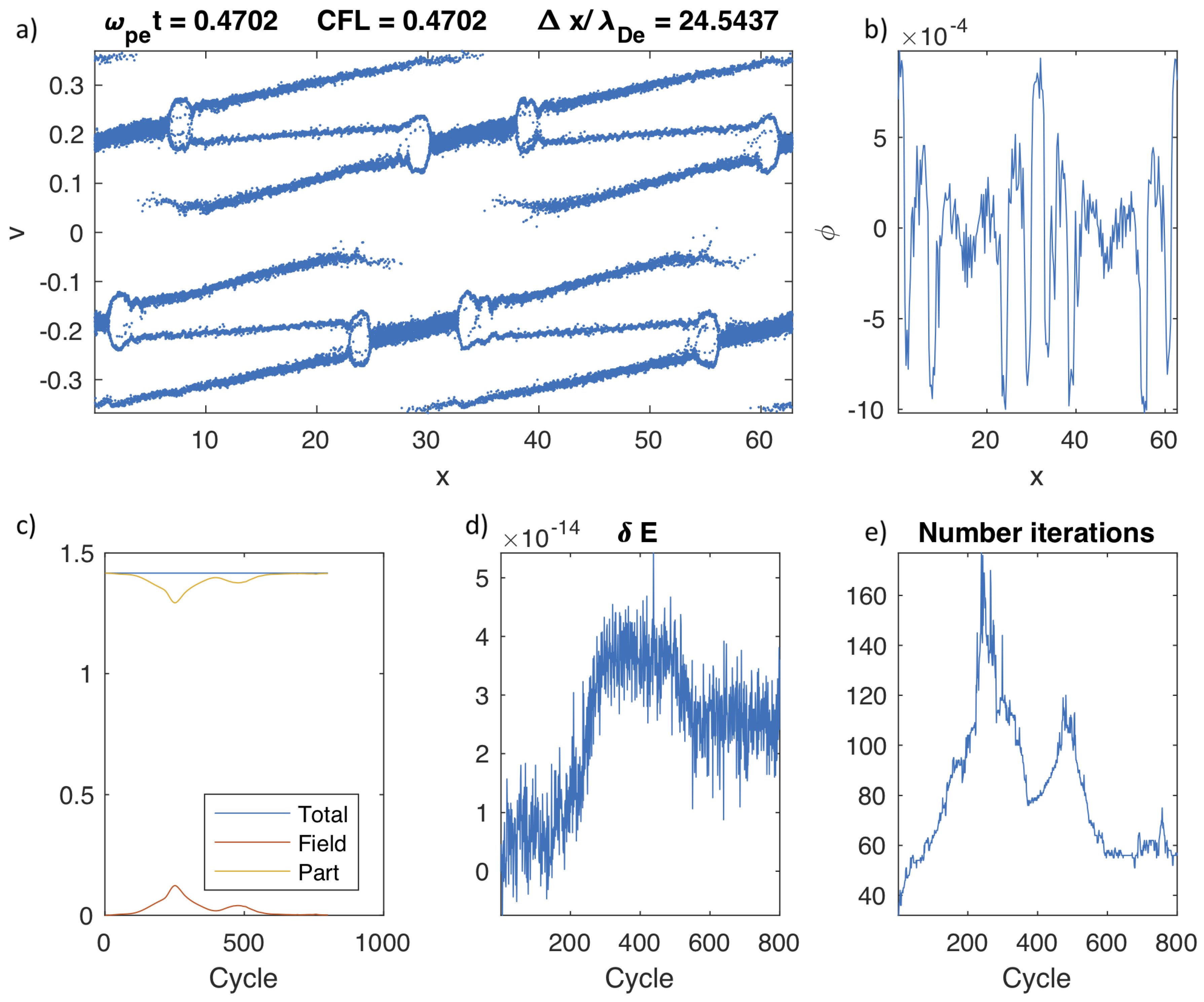
Figure 3a shows the final state of the run for Method 1. As can be observed, the evolution leads to the formation of double layers (sometimes referred to as electrostatic shocks) [27]. Figure 3b shows the electrostatic potential at the end of the run. Sharp potential jumps are present in correspondence with each shock.

The same case is repeated with Method 2 where the non-linearity of the field equations is simplified by using the potential at the n time level. Figure 4 shows the results. As can be seen, the differences in Panel a where the distribution function is shown are visible only in low detail. Similar conclusions can be reached for Panel b where the potential is also similar with the same peaks (although the structure of the peaks varies slightly). There is clearly the same amount of shock and the same patterns. The differences, however, are quite significant in terms of the number of iterations needed—the more non-linear case obviously requires more iterations.

However, is the solution correct? We have two indications that it is. First, we conducted a convergence study in which the number of cells and particles was varied. The results presented are converged in the sense that the location of the features in the phase space does not change. Second, the presence of shock-like features in conditions similar to those reported here also led to similar phase space features [27]. We therefore have confidence that the solution is correct.

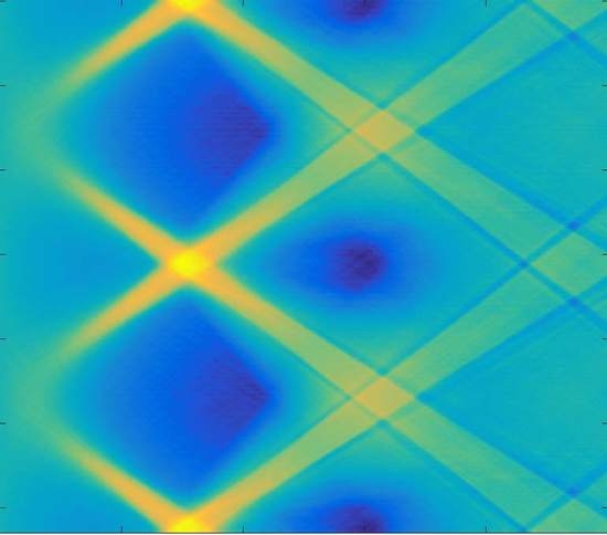
These shocks travel through the system. Figure 5 reports on both methods; for the space-time evolution, shocks can be identified by the sharp transition in the field value. The shocks move at a constant speed. The periodicity of the boundary conditions allows a shock to exit one side and re-enter the other. Shocks are also observed to interact and pass through each other.

Besides the interesting physics that were accurately resolved, the point of the test was to evaluate energy conservation. Energy is being exchanged between particles, mediums, and fields, but the total energy is exactly conserved (see Figure 3c and Figure 4c). The solution requires a tolerance in the iteration of the NK method. We set a tolerance of ${10}^{-14}$ and we indeed found energy conservation to be within the tolerance set, as shown in Figure 3d and Figure 4d. If the tolerance level is modified, so is the level of confidence in the energy conservation. Both methods considered produced exactly the same energy conservation.

For the two cases reported, the number of iterations at each cycle is shown in Figure 3e and Figure 4e. The number of iterations has a remarkable increase corresponding to the time when the shocks are first formed. Method 1, with the explicit non-linearity of the field equation, requires more iterations by a factor of approximately 50% more, a non-negligible effect.

In the above comparison of Method 1 and Method 2, we used the JFNK non-linear solver. The physical results are independent of the non-linear solver, but the computational cost of reaching those results depends on the non-linear solver used; finding the most efficient is the target of the next section.

8. Performance of Field-Hiding and Direct Newton–Schwarz

As described above, the performance of the JFNK might be increased if field-hiding or the DNS method is used. We focus now on Method 2 for two reasons. First, it was shown to be accurate and more computationally efficient in the test above. Second, it is simpler to implement field-hiding when the equations for the fields are formally linear.

The latter point requires clarification. When field-hiding is used, for each Newton iteration applied to the particles, the fields need to be computed using the current Newton iterate of the particle velocity (and indirectly, the position). This operation can be done with a linear solver if the field equations are linear, but it can also be done with another non-linear solver if the equations are non-linear. The first method nests a linear solver inside the function evaluation for the residual of the particles; the second nests a non-linear (for example, another independent JFNK) solver for the field equation. Both can be done, but of course, the first is simpler.

To evaluate the performance of the three non-linear solvers, we considered a series of progressively larger systems. The following parameters were held fixed in all runs: the time step ($\Delta t=1.25$), the grid spacing ($\Delta x=20\pi /64$) using 10,000/64 particles per cell, and the medium temperature ($e/kT=253.3030$). We changed, however, the system size by multiples M of $L=20\pi M$. We then used $10000M$ particles and $64M$ cells in each run. As M was varied, we compared the number of iterations and the total CPU time for the direct solution with JFNK including both field and particle residuals (referred to as vanilla JFNK) with that of field-hiding and DNS.

Figure 6 shows the average number of Newton iterations needed for the three solution strategies. The two methods based on the JFNK iteration performed nearly ideally, with no significant variation in the number of Newton iterations needed as M increased. The DNS performed well only for small systems—when the scaling M increased, the number of iterations ballooned and the method failed. This is due to the slow convergence caused by the approximation of the Jacobian.

The difference in iterations between FH and vJFNK is strong and compelling. The FH solution is clearly preferable.

The number of iterations correspond to a similar nearly ideal performance in CPU time for vJFNK and FH, see Figure 7. Again, the DNS loses ground on larger systems. FH results in almost an order of magnitude gain in computational time.

All tests were done on a dual Intel(R) Xeon(R) CPU E5-2630 0 at 2.30 GHz with a cache size of 15,360 KB with 64 GB RAM memory. Note that, in the analysis above, we used the same tolerance for all three non-linear solvers to enforce the exact same accuracy in all three solutions that were therefore indistinguishable from a physical point of view. The only difference was in the number of iterations and the cost of the simulation. However, the accuracy of the end results was the same. This was especially true for the DNS where the Jacobian was approximated. Approximating the Jacobian in the Newton method can slow the rate of convergence, and the direction used to compute the next guess might become sub-optimal. However, the solution obtained is still exact, it just might require more iterations.

9. Conclusions

We extended the recent developments on fully implicit energy conserving particle methods to the case where long-range forces are mediated by a medium with very different time and space scales than the inter-particle forces. This is the case for the Poisson–Boltzmann equation that describes a variety of physical systems.

We designed a new implicit method that has been shown to conserve energy exactly when rounded off. The method is based on the solution with the JFNK method of a non-linear system of equations composed by the momentum equation for each particle (Newton’s law) and the equation of the medium (Boltzmann factor included in Poisson’s equation). The challenge of the new approach is the computational cost. We investigated two strategies for reducing the number of iterations needed by hiding the field solution within the residual evaluation of the particles.

In the FH approach, the JFNK methods are still used but are applied only to the particle residual at each new Newton iteration for the particle velocities, provided the fields are computed directly (using a direct solver). This avoids the need to also include the field equations as part of the residual evaluation (a strategy referred to as field-hiding).

In the DNS approach, even the JFNK for the particles is removed. We compute analytically the Schwarz decomposed Jacobian of each particle and invert it analytically. The coupling between particles is handled as a Picard iteration. The method does not require any extra storage besides one copy of the particle information. This is a strong reduction from the JFNK approach that needs to keep in its memory multiple Krylov vectors with the same dimension of the residual (that is, the size of the number of particle unknowns).

The three methods differ only in the solution strategy and the number of iterations, but the solution is the same.

We tested our approach for the case of two ion beams moving in a medium of Boltzmann-distributed electrons, a configuration leading to multiple interacting double layers (electrostatic shocks)—a very taxing test for the methods. The field equations were discretized in two ways, one with a stronger non-linearity that assumed the medium response at the mid-time level (Method 1) and one with weaker non-linearity that treated the medium at the beginning of the time level (Method 2).

We showed both to conserve energy and to lead to virtually identical results, but the weaker non-linear discretization that evaluated the medium at the beginning of the time step had a distinct advantage.

We then focused on Method 2 and compared the JFNK approach based on including all residuals in the evaluation with FH and DNS. Both methods based on the JFNK approach showed a nearly ideal scaling, with the number of iterations remaining independent of the system size and the computational cost increasing linearly. On the other hand, the DNS started to fail as the system size increased: the number of iterations increased and the CPU time increased superlinearly.