
Machine Learning Based Restaurant Sales Forecasting


Department of Computer Science, University of New Orleans, New Orleans, LA 70148, USA
*
Author to whom correspondence should be addressed.
Mach. Learn. Knowl. Extr. 2022, 4(1), 105-130; https://doi.org/10.3390/make4010006
Submission received: 19 December 2021
/
Revised: 25 January 2022
/
Accepted: 26 January 2022
/
Published: 30 January 2022
(This article belongs to the Section Learning)
Abstract
:To encourage proper employee scheduling for managing crew load, restaurants need accurate sales forecasting. This paper proposes a case study on many machine learning (ML) models using real-world sales data from a mid-sized restaurant. Trendy recurrent neural network (RNN) models are included for direct comparison to many methods. To test the effects of trend and seasonality, we generate three different datasets to train our models with and to compare our results. To aid in forecasting, we engineer many features and demonstrate good methods to select an optimal sub-set of highly correlated features. We compare the models based on their performance for forecasting time steps of one-day and one-week over a curated test dataset. The best results seen in one-day forecasting come from linear models with a sMAPE of only 19.6%. Two RNN models, LSTM and TFT, and ensemble models also performed well with errors less than 20%. When forecasting one-week, non-RNN models performed poorly, giving results worse than 20% error. RNN models extended better with good sMAPE scores giving 19.5% in the best result. The RNN models performed worse overall on datasets with trend and seasonality removed, however many simpler ML models performed well when linearly separating each training instance.

1. Introduction
Small and medium-sized restaurants often have trouble forecasting sales due to a lack of data or funds for data analysis. The motivation for forecasting sales is that every restaurant has time-sensitive tasks which need to be completed. For example, a local restaurant wants to make sales predictions on any given day to schedule employees. The idea is that a proper sales prediction will allow the restaurant to be more cost-effective with employee scheduling. Traditionally, this forecasting task is carried out intuitively by whoever is creating the schedule, and sales averages commonly aid in the prediction. Managers do not need to know the minute-to-minute sales amounts to schedule employees. So, we focus on finding partitions of times employees are working, such as dayshift, middle shift, and nightshift. No restaurant schedules employees one day at a time, so predictions need to be made one-week into the future to be useful in the real world. Empirical evidence by interviewing retail managers has pointed to the most important forecasted criteria to be guest counts and sales dollars and that these should be forecasted with high accuracy [1]. Restaurants tend to conduct these types of predictions in one of three ways: (1) through a manager’s good judgment, (2) through economic modeling, or (3) through time series analysis [2]. A similar restaurant literature review on several models/restaurants [3] shows how the data is prepared will highly influence the method used. Good results can be found using many statistical models, machine learning models, or deep learning models, but they all have some drawbacks [3], expected by the ‘No Free Lunch’ theorem. A qualitative study was conducted in 2008 on seven well-established restaurant chains in the same area as the restaurant in our case study. The chains had between 23 and 654 restaurants and did between $75 million and $2 billion in sales. Most used some sort of regression or statistical method as the forecasting technique, while none of them used ARIMA or neural networks [4]. ARIMA models have fallen out of favor for modeling complex time series problems providing a good basis for this work to verify if neural network research has improved enough to be relevant in the restaurant forecasting environment.
In the modern landscape, neural networks and other machine learning methods have been suggested as powerful alternatives to traditional statistical analysis [5,6,7,8,9]. There are hundreds [10] of new methods and models being surveyed and tested, many of which are deep learning neural networks, and progress is being seen in image classification, language processing, and reinforcement learning [5]. Even convolutional neural networks have been shown to provide better results than some of the ARIMA models [6]. Traditionally, critics have stated that many of these studies are not forecasting long enough into the future, nor do they compare enough to old statistical models instead of trendy machine learning algorithms. Following, machine learning techniques can take a long time to train and tend to be ‘black boxes’ of information [10]. Although some skepticism has been seen towards neural network methods, recurrent networks are showing improvements over ARIMA and other notable statistical methods. Especially when considering the now popular recurrent LSTM model, we see improvements when comparing to ARIMA models [8,9], although the works do not compare the results with a larger subset of machine learning methods. Researchers have recently begun improving the accuracy of deep learning forecasts over larger multi-horizon windows and are also beginning to incorporate hybrid deep learning-ARMIA models [7]. Safe lengths of forecast horizons and techniques for increasing the forecasting window for recurrent networks are of particular interest [11]. Likewise, methods for injecting static features as long-term context have resulted in new architectures which implement transformer layers for short-term dependencies and special self-attention layers to capture long-range dependencies [5].
While there has been much research using the old ARIMA method [12,13] for restaurant analysis, in this paper, we aim to broaden modern research by studying a wide array of machine learning (ML) techniques on a curated, real-world dataset. We conduct an extensive survey of models to compare together with a clear methodology for reproduction and extension. An ML model is ideally trained using an optimal number of features and will capture fine details in the prediction task, such as holidays, without underperforming when the forecast window increases from one day to one week. We describe the methodology required to go from a raw dataset to a collection of well performing forecasting models. The purpose is to find which combination of methodologies and models provide high scores and to verify whether state-of-the-art recurrent neural network architectures such as LSTM, GRU, or TFT, outcompete traditional forecasting ML models such as decision trees or simple linear regression. The results add to the landscape of forecasting methodologies tested over the past 100 years, and suggestions for the best methods for the data are given in the conclusion.
2. Literature Review
The comparison of ML techniques to forecast curated restaurant sales is a common research question and can be seen in several recent works [14,15,16,17]. Two additional recent, non-restaurant forecasting with ML problems are also examined [11,18]. Although similar in model training and feature engineering techniques, our methodology differs from other recent forecasting papers in a few key areas, which we outline. The first important difference in researched methods is the forecasting horizon window used. Many papers either used an unclear horizon window or made forecasts of only one time step at a time [14,15,16,17,18]. Only one paper increased the forecast horizon beyond one time step [11], so we consider forecasting one week of results the main contribution of this research. Another point of departure with reviewed papers is the importance of stationary data. Traditionally, it is important to have a stationary dataset when working with time series so there is no trend or seasonality learned—instead, each instance is separated and can be forecasted based on its own merit instead of implicit similarity. However, only one paper [11] even mentions this stationary condition. Instead of exploring it further, the authors simply trained models using data that did not seem to have any associated trend. As an extension to these works, we consider the stationary condition and test multiple datasets to gauge its importance. The main departure in this study from the other literature is the engineering of weather as a feature in the feature-set. All but one paper [11] includes the modeling of weather as feature labels for forecasting, although we refrained from including this in our own research. Even though not present in the work, we may consider weather as a potential future enhancement to try and improve results further. The premiere difference, which we aim to highlight in this work, are the models selected for testing. Some papers test only traditional models such as linear regression, decision trees, or support vector machines [15,16,17] with no mention of recurrent neural networks (RNN). One paper only includes RNN models without any other family of statistical or ML models for comparison [11]. The final two papers include a mix of models; however, the collection of RNN and traditional models are small [14]. Not one paper includes results for the new TFT model first published in 2020, which is featured heavily in this work. Compared to these papers, we test a larger number of RNN and ML models for a more robust comparison.
3. Materials and Methods
In this section, we outline the methodology used in this work. We begin with the acquisition and preprocessing of the datasets for the case study, which were initially curated for use as the main contribution in the author’s master thesis [19]. Methods of partitioning, feature selection, and differencing are studied uniquely for this data but also are listed as general techniques to follow for other similar problems or datasets. We briefly list all the methods used for the forecasting task. Each model goes through a specific training pipeline which will be described in some detail. Next, we describe the recurrent neural network architectures used in this work in enough detail to provide context for those unfamiliar. Following, we describe the metrics used in this study to compare the various modeling techniques employed. Finally, we discuss how models are compared against common baseline approaches, filtered to acquire the best feature subset, then tested to acquire our final results.
3.1. Data Acquisition
The raw data was collected in three chunks ranging from 8 September 2016–31 December 2016, 1 January 2017–31 December 2017, and 1 March 2018–5 December 2019. Restaurants gather customer information through a point of sale (POS) system, which catalogs a wide array of information, including the time, items sold, gross sales, location, customer name, and payment information such that each sale made provides a unique data point. While there is plenty of interesting information to mine from the raw data, we have narrowed down our interest to just the gross sales, date, and time. For each data dump, we extract the three previously mentioned features. The time is recorded down to the second, so every item sold within an hour is easily aggregated together. Likewise, it is a simple task to group all hours of sales from a single day from 10:00 a.m. to 10:59 p.m., as seen in Figure 1. Thus, by this stage, we have processed each day of gross sales into an instance of 12 h and date. We may then consider how partitions of hours will aid in the completion of the forecasting task. To simplify the forecasting problem, we bin the daily sales into three partitions from 10:00 a.m. to 1:59 p.m., 2:00 p.m. to 5:59 p.m., and 6:00 p.m.to 10:59 p.m., as shown in Figure 2. Instead of predicting an entire day, we will train a model to predict just one partition. The focus of this work is forecasting the middle partition from 2:00 p.m. to 5:59 p.m., although the same methods can be used on the remaining partitions.
We are missing data in two sections. The first is a large gap from 31 December 2017 to 1 March 2018, missing 58 days. The second gap misses 5 days from 31 May 2019 to 5 June 2019. In total, this is 63 days of missing data, and we do not have a continuous dataset. Losing a few data points should not cause too much confusion if the issue is addressed correctly [20], although care is needed. Restaurant sales are heavily influenced by weekly seasonality, and if a day is removed, the weekly structure will be off track for the rest of the series. A full week must be extracted to preserve our structure whenever a day is missing to combat this issue. In other words, all gaps in the data must come as a multiple of 7. To this end, our first gap is extended to 31 December 2017 to 5 March 2018 for 63 days of missing data, and the second is extended to 31 May 2019 to 5 June 2019 for 7 days of missing data. This method is known as listwise deletion and is considered an ‘honest’ approach to handling missing data [21]. In total, we have 70 days of unrecorded missing data, but the weekly seasonality is held.
3.2. Additional Stationary Datasets
Popular, traditional methods of statistical forecasting, such as ARIMA models, are known to require a dataset that is stationary. That is, the mean and variance should be approximately the same across the dataset. To this end, trend and seasonality within the dataset must be removed [20,22]. Although this work does not feature ARIMA models, we aim to see if stationary datasets might improve the results of machine learning and RNN techniques. We have a positive trend as the restaurant has increased sales over the years, and a clear seasonality of one week is seen convincingly in Figure 3.
To remove trend and seasonality to create a stationary dataset, we employ a technique called differencing [23]. We will no longer be predicting the actual sales amount but the difference in sales from the previous time-period. Differencing is allowed for any time window, although most often, we difference D (t) with previous day D (t − 1). We study two differencing windows in detail: daily difference D (t − 1) and weekly difference D (t − 7). If necessary, it is possible to increase the order of the difference by differencing the data as many times as desired. We obtain a daily difference (Equation (1)) instead of the actual sales between 2 p.m. and 5 p.m., and we take the difference of sales such that,
Once differencing has been completed, we review our data, shown in Figure 4, and see there is less of an obvious upward trend. We check for seasonality with the correlation plot in Figure 5, and we see that there is still a weekly correlation that has not been removed. This correlation outside the confidence zone suggests that we have not completely removed seasonality from our data. Although, more days in total reside outside of the confidence zone than in Figure 3, meaning we may gain some additional information from negative correlation. The amount of MAE generated when forecasting over a differenced dataset is equivalent to the MAE generated when mapping back to its pre-transformed shape, so the MAE scores are directly comparable.
Similar to daily differencing, we may now define the dataset using the weekly difference Equation (2) instead of the actual sales. We take the difference such that,
From Figure 6, we again view that the trend has been differenced out of our dataset. Let us also verify with Figure 7 that the weekly correlation has been removed. When reviewing the figure, we see that all but seven days in the past have had correlation removed to the point that they can be considered ‘not correlated.’ Presumably, there will be no assumptions made by our models about seasonality, which makes for a prediction not dominated by average results.
3.3. Feature Definitions
We identify all features used in the training process. Some features are easily mined from the raw data, some features are generated from summary statistics, and some features come from outside the dataset—such as special holiday events. It is of note that we do not use weather metrics as feature labels in favor of testing holidays and summary statistics on their own merit, although this is generally accepted as a very good method for increasing forecast accuracy [14,15,16,18]. We define or otherwise summarize all features in Table 1.
3.4. Considered Models
For a full and robust comparison of models, we conduct a survey of 23 different machine learning models and two baseline predictors which are shown in Table 2. The models range in complexity from simple linear models to the advanced Temporal Fusion Transformer model (TFT). Table 2 also provides references to the supplemental document for more detail on models, which include a meta structure to be defined, such as the number of hidden layers in our recurrent neural network (RNN) models or the models used in ensemble methods. We provide further reading resources for all models in the table but will take some time to describe RNNs as these include the most novel models tested.
We focus discussion on neural networks, which do not only include a simple feed-forward prediction method. Instead, recurrent neural networks (RNNs) create short-range time-specific dependencies by feeding the output prediction to the input layer for the next prediction in the series. This design philosophy has been popular since the late ’90s and has been used for financial predictions, music synthesis, load forecasting, language processing, and more [12,64,65]. The most basic RNN form may be modeled with the idea that the current hidden state of the neural network is dependent on the previous hidden state, the current input, and any additional parameters of some function, which we show as Equation (3). RNN models are trained with forward and backwards propagation [66].
By building on the ideas of Equation (3), we allow for many flavors of the RNN model. These recurrent layers can be supplemented with convolutional layers to capture non-linear dependencies [6]. To further improve performance, special logic gates are added to the activation functions of the recurrent layers, which have mechanisms to alter the data flow. Encoding/decoding transformer layers, which take variable-length inputs and convert them to a fixed-length representation [61], have also shown good results. These layers integrate information from static metadata to be used to include context for variable selection, processing of temporal features, and enrichment of those features with the static information [5]. Another augmentation is a special self-attention block layer, which finds long-term dependencies not easily captured by the base RNN architecture [5].
This work highlights four models using a recurrent architecture. The first is a simple RNN model without any gating enhancements. While RNN models have proven successful in many disciplines, the models struggle to store information long-term [13], and the model is known to be chaotic [58] due to vanishing or exploding gradients [59]. To aid in the gradient problem, the LSTM and GRU neural networks have been developed. Both architectures are specific cases [12] or otherwise modified from the base RNN model by the addition of gating units in the recurrent layers. Some studies have been completed, suggesting that LSTMs significantly improve retail sales forecasting [9].
The long short-term memory (LSTM) network was developed with the idea of improving the RNN’s vanishing/exploding gradient problems in 1997 [60] and is better at storing and accessing past information [13]. The mechanism used is a self-looping memory cell which produces longer paths without exploding or vanishing gradients. The LSTM memory cell is comprised of three gates, an in-gate, an out-gate, and a forget-gate. These gates all have trainable parameters for the purpose of controlling specific memory access (in-gate), memory strength (out-gate), and whether a memory needs to be changed (update-gate) [66]. The main state unit, , is a linear self-loop weighted directly by the forget unit, , shown as:
where is the current input, is the bias, the recurrent weights, and the input weights. This value is scaled between 0 and 1 by the σ unit. The internal state is then updated as:
The external gated unit,, is calculated in the exact same manner as Equation (5), although the unit uses its own set of parameters for biases, input weights and, forget-unit gates. Finally, we concern ourselves with the output of the LSTM hidden layer as,
The output gate is influential and may even cut off all output signals from the memory unit and has parameters for the biases, input weights, and recurrent weights as defined in the other gates. Although LSTM models have shown success in forecasting, the next extension to RNNs questions if all three gates are necessary for training a strong model.
Next, the gated recurrent unit (GRU) model is another type of recurrent neural network implementing memory cells to improve the gradient problem and was proposed in 2014 by Cho et al. as a convolutional recursive neural network with special gating units [61]. The GRU model is very similar to the LSTM model but removes the combines the forget-gate with the update-gate [66] with the idea that fewer parameters to train will make the training task easier—although we lack fine control over the strength of the memory being fed into the model [62]. The states for a GRU cell can be updated as follows:
where u and r are update and reset gates and the values are calculated similarly as seen for LSTMs as:
In addition,
In the year 2019, authors Lim et al. released the temporal fusion transformer (TFT) network, a novel, attention-based learning architecture that combines high-performance multi-horizon forecasting with interpretable insights into temporal dynamics [5]. We give a brief description of the TFT model as an introduction as the model architecture is laid out in sufficient detail in the preliminary paper titled Temporal Fusion Transformers for Interpretable Multi-horizon Time Series Forecasting.
The TFT architecture uses a direct forecasting method [7] where any prediction has access to all available inputs and achieves this uniquely by not assuming that all time-varying variables are appropriate to use [5]. The main components of the architecture are gating mechanisms, variable section networks, static covariant encoders, a multi-head attention layer, and the temporal fusion decoder. The authors propose a gating mechanism called Gated Residual Network (GRN), which may skip over unneeded or unused parts of the model architecture. Variable selection network ensures relevant input variables are captured for each individual time step by transforming each input variable into a vector matching dimensions with subsequent layers. Each static, past, and future inputs acquire their own network for instance-wise variable selection. Static variables, such as the date or a holiday, are integrated into the network through static enrichment layers to train for temporal dynamics properly. The static covariant encoder integrates information from static metadata to be used to inform context for variable selection, processing of temporal features, and enrichment of those features with the static information [5]. Short-term dependencies are found with LSTM layers, and long-term dependencies are captured with multi-headed self-attention block layers. An additional layer of processing is completed on the self-attention output in the position-wise feed-forward layer. This process is designed such as the static enhancement layer. The practical difference gained from the advanced architecture is that the RNN, LSTM, and GRU models must make long-term forecasting decisions from a single instance, while the TFT model can use future instances while hiding unknown information—such as the forecasting target. The drawback for generating this context with such a large architecture, making use of many layers, is the abundance of hyper parameters to be tuned.
3.5. Metrics
The metrics officially used to evaluate our models’ accuracy are the mean absolute error (MAE), defined below in Equation (11), the symmetric mean absolute percent error (sMAPE) in Equation (12) and the geometric mean absolute error (gMAE) in Equation (13).
where n is the number of instances being predicted, and y is each instance. When listing the MAE, we always cut off the decimal and keep the whole number for ease of notation. We take the MAE because positive errors and negative errors have a similarly negative effect. The MAE also provides a simple way to discuss the results because the target directly relates to the sale values. When we have an MAE of 50, we may directly say that our prediction was incorrect by $50.00. sMAPE is a useful, balanced way to verify the mean percentage of error for our forecast result. We use symmetric-MAPE because the basal MAPE formula places only the absolute value of ytrue into the denominator, which gives the restriction that no instance may be 0 or the result will be undefined. Different implementations of the metric may ignore the label entirely or give the largest possible error. Either way, this creates an inconsistency in testing, and this is a problem because there are exactly three instances in our dataset with an actual value of 0. sMAPE is slightly improved because the formula will only be undefined in the case that ytrue = ypred = 0. Although rare, we will point out situations where this may occur, and the sMAPE value may be slightly smaller than actually recorded for those instances. The gMAE is another metric often used when researching time-series and tends to be most appropriate for series with repeated serial correlation, which makes this suitable for our needs. gMAE does have similar problems as seen in sMAPE, and 0-valued errors are handled by adding a small amount of noise to the returned value whenever the error calculated is 0.
3.6. Baselines
A simple method of predicting sales is by using the previous instance as the prediction. The instance window may be daily, weekly, or any real value to use as ‘lag’, but there is no additional logic. Naïve solutions are easy to implement and are often discussed in introductory forecasting texts [23], and may be easily adopted in real-world practice. So, we analyze the MAE and MAPE scores of Use-Yesterday (Equation (14)) and Use-Last-Week (Equation (15)) for use as a baseline result. Naïve solutions are not always reliable, so to improve our baseline, consider the average sales found for a particular sales day. The lag used is the previous weekday D (t − 7), and the moving average window is the entire dataset preceding D (t) that belongs to the same weekday (i.e., only Mondays) seen in Equation (16).
where is the current prediction, y is actual, and n represents the total number of weeks preceding t. As an example of Equation (16), a prediction for Saturday would be a mean result between last Saturday’s sales and historical average Saturday sales. The dataset’s full average values are used but using a rolling moving average window to contextualize current trends is another common approach.
3.7. Feature Selection
With so many features derived from the data, it may be the case that some are useless or even harmful to some models. To reduce noise from unnecessary features, we conduct a special univariant feature test to test each features importance individually. First, we rank the features from greatest importance to least important by scoring each feature individually. The feature-ranking is conducted using a quick univariant linear regression model to find Pearson’s correlation coefficient between each regressor and the target to calculate the p-value as seen in Equation (17). The correlation is then converted to an F-score, a test of statistical relevancy where the higher the score, the more relevant the feature is to the forecast, shown in Equation (18), and is bounded by (0, infinity).
Second, we generate MAE scores for each model by training on an iteratively increasing number of n ranked features from 1 to k, where k includes all features. From this test, we find the optimal number of features per model and estimate the final MAE score. For one-day forecasting, it is easy to use univariant testing techniques to estimate feature importance, although nuance from co-correlation between features may be lost. For one-week forecasting, we use the same importance found for the one-day forecast.
The TFT model is the only model which does not go through the entire feature selection test as tuning the model takes many hours to complete. As such, an estimate of the best feature set is selected from the results of the LSTM model test, and this subset of features is used for tuning. To ensure we are acquiring an improved score, we also tune a TFT model on the same dataset with the full feature list. These hyper-parameters, the values of which may be found in Supplementary Materials Tables S4–S8, are then used in final training.
3.8. Model Train/Test Set
To standardize comparisons between models, we designate a testing dataset. One-day forecasting uses the final 221 days of instances, and one-week forecasting uses the final 224 days of testing. One-week forecasting uses a sliding window to predict seven days at a time, so we can test different starting points to show which models are stable when beginning predictions on different days of the week. The test set is not sorted or otherwise altered, and we create testing sets for the actual, daily differenced, and weekly differenced sales datasets. Respectively, the shapes can be seen as Supplementary Materials Figures S6–S8, and an example of the one-week forecast test data is seen in Supplementary Materials Figure S9. The goal of each model will be to forecast these lines to its best ability.
3.9. Complete Model Learning Methodology
We outline the full learning process now that the relevant pieces have been defined. The full outline can be followed in Figure 8. First, the raw dataset is collected. Preprocessing steps are completed to generate all features and to create the different datasets. For the three datasets, we complete feature tests, optimizing the MAE score, with all models to evaluate the best number of features for training. The top eight non-recurrent models and all recurrent models are considered candidate models for each dataset. A train/test split is used for the final training where the candidate models are trained using all available data not used in the baseline test. Models are trained by optimizing the MAE score in the final training. We then use our models to forecast the testing datasets to make final comparisons using our pre-defined metrics.
4. Results
In this section, we give the best-found results from our test suites. First, we show the baseline scores used for comparisons. Then, we discuss the results of the feature test and which models scored high enough to be candidate models. Following, we include the final top 25 results for one-day forecasting and the increased horizon one-week forecasting. Supplementary Materials will be pointed out throughout the results section in case readers wish to compare forecast shapes and scores of models not in the top 25 results. Results from all three datasets are included for direct comparison.
4.1. Baseline Results
In Figure 9, we see the actual value in blue with our prediction line in orange. The mean absolute error (MAE) score for the Use-Yesterday prediction is 403. Our data is correlated weekly instead of daily, which yields a high error. This does show the upper bounds prediction error, so it is a simple goal to achieve better results. In Figure 10, we see the result of the Use-Last-Week prediction on the test dataset. The MAE score for Use-Last-Week prediction is 278. As expected, we see a large increase over the previous baseline due to the weekly seasonality, and we consider this to be a well-reasoned prediction. There are issues regarding zero-sale days as they propagate errors forward.
In Figure 11, we see the result of the Use-Last-Week-Enhanced prediction. The MAE score for the prediction is 239 showing a large improvement over simpler baselines and is even sensitive to change over time as short-term increases or decreases will be caught by the next week. This simple model boasts a sMAPE of 21.5%, which is very good. Although it is sensitive to changing patterns, the prediction will never propagate error from a holiday forward as badly as the other baselines.
4.2. Feature Test Results
Figure 12 shows the rankings of the top 25 features in the actual dataset and their associated F-Scores. This ranking step is completed for each of the actual, daily differenced, and weekly differenced datasets, and the results can be seen in the Supplementary Materials Figures S10–S12. Since the Temporal Fusion Transformer (TFT) model injects static context and does not need the 14 days of previous sales, we also give the top feature rankings with the 14 days removed in Supplementary Materials Figures S13–S16. Examining the results of the actual dataset, we see by far the most highly correlated features are the weekly average sales, the sales from one week ago, and the sales from two weeks ago. One feature of note, the year scores high, even though predicting sales by the year is not a good metric in reality. Since the actual dataset has a built-in trend, the feature seems more contextual than it really is. The daily differenced dataset, which has successfully removed trend, shows the highest scoring features as Monday and Saturday, as well as sales from one and two weeks ago as before. Although scores are not at high as before, there is still a good correlation, and features relying on trends do not rank highly such as before. Finally, the weekly differenced rankings show further diminished F-Scores. Sales from the day one week prior remain a consistent, highly correlated feature. Since the most correlation between instances has been removed by weekly differencing, holidays are ranked more highly than most other features.
The test to find the optimal number of features is completed for each model on each of the actual, daily differenced, and weekly differenced datasets for one-day and one-week forecast horizons. First, we examine the one-day results, followed by the extension to one-week. Figures for one-day results beyond the actual dataset can be seen in Supplementary Materials Figures S16–S21. The one-day actual feature test, shown in Figure 13, shows very promising results for the RNN models with LSTM using 22 features and GRU using 10, both scoring higher than other models. Other than some ensemble and linear non-RNN methods, most models received the highest MAE score from a smaller number of features on the actual dataset due to the high correlation of just a few features. This behavior is seen clearly in Figure 14 where all RNN models perform much worse after selecting more than 20 features. The one-day daily differenced feature test shows worse MAE scores overall, and the RNN models perform severely worse. Due to daily differencing linearly separating each instance, the best performing models may make use of more features. Kernel Ridge regression with 72 features received the best MAE in this stage and is comparable to the best results in the actual dataset. Ridge regression steadily decreased in MAE as the features increased, but RNN models fluctuated with an upward trend instead of improving, giving the best results with fewer features. The final weekly differenced one-day feature test gives steadily worse results for all models, and the RNN models are outperformed again by most other ML methods. For most models, except for some tree-based methods, the MAE never decreases beyond adding a small sampling of features, around 14 features for many models. For one-day feature testing, we acquire the best results overall from the actual data using few features and daily differenced data using many features, with the weekly differenced results underperforming overall with a middling number of features.
The one-week feature tests are comparable to the one-day tests in many cases, and the resulting figures can be examined in detail in the Supplementary Materials Figures S22–S27. Due to forecasting for seven time steps instead of just one, we acquire slightly higher MAE results overall. For the actual dataset, the LSTM model is still the best, with only 24 features included, and both GRU models performed very well. All high-scoring, non-recurrent models find the best results with an increased number of features, 60 or more in most cases. Although we observe a high correlation in features, most of the correlation is only useful for the t + 1th position, and the models need additional features to help forecast the remaining six days. Other than higher overall MAE scores and more features used on average, the results from the one-week feature test are very similar to the one-day results.
4.3. One-Day Forecasting Results
The best model for forecasting one-day into the future implements the kernel ridge algorithm with a test MAE of 214, sMAPE of 19.6%, and a gMAE of 126, although all 25 top models are shown in Table 3. The dataset used was the daily differenced dataset, and the forecast result is seen in Figure 15. This is the best individual MAE score among all models. The TFT model with fewer features forecasted over the actual dataset also did well with an MAE of 220, sMAPE of 19.6%, and a gMAE of 133. This model better captures special day behaviors but is less adaptive since it uses fewer features. The ensemble Stacking method also received good results using the actual dataset, making it comparable to the TFT model. Otherwise, many models outperformed the best Use-Last-Week-Enhanced baseline. When examining datasets, daily differencing consistently achieves scores higher than the actual or weekly differenced dataset, especially with linear models. RNN models require the actual dataset to achieve results which are better than the baseline and still perform worse in some cases. The actual dataset still achieves below baseline results with other ML models as well; they are just not as good as seen when differencing daily. Finally, the weekly differenced dataset provides results almost entirely worse than the baseline, with the best result coming from the Voting ensemble. The full table of test results with all models is given in the Supplementary Materials Table S9, and we give some figure examples from high performing or interesting forecasts in Supplementary Materials Figures S28–S35.
4.4. One-Week Forecasting Results
When reviewing Table 4, the best model MAE score over one-week is the TFT model with fewer features achieving an MAE of 219, sMAPE of 20.2%, and a gMAE of 123 using the actual sales dataset. The forecast, seen in Figure 16, shows a perfect capture of the two holidays. However, the GRU and LSTM models both achieve a better sMAPE of 19.5% and 19.7%, respectively, and they both have better gMAE scores. The GRU model is hindered by a very high deviation between the starting days, and a Sunday start gave the best results. No other results achieved better scores than the Use-Last-Week-Enhanced baseline. The best performing non-recurrent models were ensemble methods Extra Trees, Stacking, and Voting, all on the actual dataset. When examining datasets, the only results better than the baselines came from the Actual dataset. Although, it is likely most accurate to say that only our recurrent algorithms performed well, and the actual dataset is the only one conducive for training recurrent models. The weekly differenced dataset does perform better than the daily differenced dataset here in terms of MAE, although the sMAPE is massive. Examining the forecasts shows models which are predicting close to zero-difference to achieve results approaching the Use-Last-Week baseline, which explains decent MAE but high sMAPE. The daily differenced dataset is not capable of making good predictions when using this forecasting method on a long window. The best result is the Lasso model with only an MAE of 280, sMAPE of 101.6%, and a gMAE of 162. The full table of test results with all models is given in the Supplementary Materials Table S10, and we give some figure examples from high performing or interesting forecasts in Supplementary Materials Figures S36–S43.
5. Conclusions
Although one-day forecasting was exhaustively studied, the ultimate goal of this research is to find a scalable model for prediction horizons of at least one week for use on real-world data. Three datasets were tested using over 20 models to show the impact of creating stationary datasets on the feature engineering and model training processes. In the end, recurrent neural network (RNN) models performed better than other models, with the Temporal Fusion Transformer (TFT) model showing interesting results due to static context injection. TFT only performed slightly worse in one-day forecasting when compared to the best performing ridge regression model using the daily differenced dataset, but with current methods, the ridge model could not scale to one-week forecasting. While other models performed well with the differenced datasets, the RNN models struggled to provide good results in either one-day and one-week testing, so it is not recommended to use differencing techniques. While results cannot state that kernel ridge and related algorithms had good results for one-week forecasting, it is likely that a stepwise forecast, instead of predicting the full week at once, would improve the one-week forecast MAE to match more closely with one-day predictions. The same conjecture can be made for all poor one-week results. Even when learning on the previous 14 days of targets, a single instance just does not give enough context to allow great forecasts that far into the future in one step. Transformer encoding and decoding learning layers show potential for improvements in forecasting problems. Experiments with transformer-based models on different and larger datasets would be a very relevant way to continue with future work. For instance, this work only includes a single restaurant location, which provides a narrow amount of data. Similarly, machine learning models show very promising results with one day testing, and future studies on extending the forecasting window could be beneficial, as linear models are fast and simple to train. Ridge may be useful in providing one-step predictions to be used as some stepwise prediction in a longer forecast window. Similarly, as ensemble methods provided good results, it may be worth allowing linear models to predict single-step sequences of daily differences in sales for use as feature labels when training and forecasting TFT models. Further research on the TFT model is appropriate as the technology is new, and few papers have been written on it specifically. To improve results further, we may begin research on identifying safe forecasting windows to increase the accuracy of sales farther into the future. One specific method identified in [11] is to break up a long forecast window into multiple smaller, safe windows for higher prediction accuracy. Weather is also well-known to improve forecasting results, especially in retail and restaurant domains, which gives a clear path to try for future improvements in our feature engineering pipeline. Including weather, any non-static data could be used in training and then filtered out, which may allow for interesting and novel combinations of features and techniques. With our research, we have shown that the enhancements added to the TFT model over basal RNN models allow multi-horizon predictions well into the future. Other models made comparable results in one-day and one-week forecasting, but no other model can as reliably forecast zero-sale days, such as holidays, from only a few samples. Even though the TFT model was outperformed in single one-day forecasting, the ability to give or withhold context at key moments provides for more robust predictions which scale better into the future.
Supplementary Materials
The following are available online at https://www.mdpi.com/article/10.3390/make4010006/s1, Figure S1: RNN Layer Structure. The implemented RNN structure for all tests. Figure S2: LSTM Layer Structure. The implemented LSTM structure for all tests. Figure S3: GRU Layer Structure. The implemented GRU structure for all tests. Figure S4: GRU+ Layer Structure. The implemented GRU+ structure for all tests. Figure S5: General TFT Model Structure. We build six TFT models, but all use this same layer structure. Some layers are static and have no trainable parameters, while the rest will have a variable number of parameters defined by a hyperparameter tuning process. Table S5: Hyperparameter Tuning One-Day Results (Full Feature Set). Shown are the results for one-day forecasting from all three datasets using the full feature set. In addition, the best result’s loss and the number of trainable parameters are included. Supplementary Figure S6: Shape of Test Data: Actual. The shape of our test dataset was used for all one-day actual forecasting test tasks. Included are 221 days of sales from the very end of the full dataset. Supplementary Figure S7: Shape of Test Data: Daily Difference. The shape of our test dataset used for all one-day daily differenced forecasting test tasks. The test set includes 221 days of sales differenced (2) from the very end of the full dataset. Once a forecast is made, we easily transform back to Figure S6. Supplementary Figure S8: Shape of Test Data: Weekly Difference. The shape of our test dataset was used for all one-day weekly differenced forecasting test tasks. The test set includes 221 days of sales differenced (3) from the very end of the full dataset. Once a forecast is made, we easily transform back to Figure S6. Supplementary Figure S9: One-Week Test Set (Start Day Tuesday). The one-week forecasting test set uses a sliding weekday start window. Each day of the week is used as the start for seven tests. The test sets are increased by three to a total of 224 instances, which allows for an exact number of one-week predictions. An additional zero sales holiday is shown at the beginning. Predictions starting on Tuesday are shown as an example. Figure S10: F-score for Top Features (Actual). The top 25 features as ranked by their F-scores. Weekly sales average is the highest scoring feature by far with other statistical metrics and days of the week following. Figure S11: F-score for Top Features (Daily Differenced). The top 25 features as ranked by their F-scores. The day of the week and some statistical measures are high-ranking features here. Some impactful holidays also are in the top 25. Figure S12: F-score for Top Features (Weekly Differenced). The top 25 features as ranked by their F-scores. Only the previous week’s sales have a F-score above 100. Only one statistical feature remains at the top, and the most relevant features are holidays. Figure S13: F-score for Transformer Top Features (Actual). The top 25 features as ranked by their F-scores. With temporal associations built by the model, feature selection can be completed without considering lookback days specifically. Figure S14: F-score for Transformer Top Features (Daily Difference). The top 25 features as ranked by their F-scores. With temporal associations built by the model, feature selection can be completed without considering lookback days specifically. Figure S15: F-score for Transformer Top Features (Weekly Difference). The top 25 features as ranked by their F-scores. With temporal associations built by the model, feature selection can be completed without considering lookback days specifically. Figure S16: Best One-Day Forecast MAE Found Across 73 Features (Actual). Recurrent (orange) and non-recurrent (blue) models are trained with an iteratively increasing number of ranked features, seen in Supplementary Figure S10, for one-day forecasting. The lowest MAE for each model is recorded with the number of features next to the model’s name. Figure S17: All RNN Models and Ridge One-Day Forecast MAE Across 73 Features (Actual). We show how the number of features affects the MAE score for one-day forecasting in the actual dataset. Figure S18: Best One-Day Forecast MAE Found Across 77 Features (Daily Difference). Recurrent (orange) and non-recurrent (blue) models are trained with an iteratively increasing number of ranked features, seen in Supplementary Figure S11, for one-day forecasting. The lowest MAE for each model is recorded with the number of features next to the model’s name. Figure S19: All RNN Models and Ridge One-Day Forecast MAE Across 77 Features (Daily Difference). We show how the number of features affects the MAE score for one-day forecasting in the daily differenced dataset. Figure S20: Best One-Day Forecast MAE Found Across 77 Features (Weekly Difference). Recurrent (orange) and non-recurrent (blue) models are trained with an iteratively increasing number of ranked features, seen in Supplementary Figure S12, for one-day forecasting. The lowest MAE for each model is recorded with the number of features next to the model’s name. Figure S21: All RNN Models and Ridge One-Day Forecast MAE Across 77 Features (Weekly Difference). We show how the number of features affects the MAE score for one-day forecasting in the weekly differenced dataset. Weekly differenced dataset shows little improvement as features are added. Figure S22: Best One-Week Forecast MAE Found Across 71 Features (Actual). Recurrent (orange) and non-recurrent (blue) models are trained with an iteratively increasing number of ranked features, seen in Supplementary Figure S10, for one-week forecasting. The lowest MAE for each model is recorded with the number of features next to the model’s name. It is promising that most RNN models perform well in this stage, but we are wary of overfitting. Figure S23: All RNN Models and Ridge One-Day Forecast MAE Across 71 Features (Actual). We show how the number of features affects the MAE score for one-week forecasting in the actual dataset. Figure S24: Best One-Week Forecast MAE Found Across 74 Features (Daily Difference). Recurrent (orange) and non-recurrent (blue) models are trained with an iteratively increasing number of ranked features, seen in Supplementary Figure S11, for one-week forecasting. The lowest MAE for each model is recorded with the number of features next to the model’s name. Figure S25 All RNN Models and Ridge One-Week Forecast Across 74 Features (Daily Difference). The ridge example shows how the number of features affects the MAE score for one-week forecasting in the daily differenced dataset. Figure S26: Best One-Week Forecast MAE Found Across 74 Features (Weekly Difference). Recurrent (orange) and non-recurrent (blue) models are trained with an iteratively increasing number of ranked features, seen in Supplementary Figure S12, for one-week forecasting. The lowest MAE for each model is recorded with the number of features next to the model’s name. Good results from RNN models are promising, but need to be verified in a fair final test. Figure S27: All RNN Models and Ridge One-Week Forecast Across 74 Features (Weekly Difference). The ridge example shows how the number of features affects the MAE score for one-week forecasting in the weekly differenced dataset. Figure S28: Stacking Actual One-Day Forecast. MAE of 220, sMAPE of 19.5%, and a gMAE of 142, with 25 features. Figure S29: Extra Trees Actual One-Day Forecast. MAE of 231, sMAPE of 20.4%, and a gMAE of 128, with 29 features. Figure S30: Kernel Ridge Daily Differenced One-Day Forecast. MAE of 214, sMAPE of 19.6%, and a gMAE of 126, with 72 features. Original predictions (first) and then transformed back version (second) are both shown. Figure S31: Voting Weekly Differenced One-Day Forecast. MAE of 238, sMAPE of 21.3%, and a gMAE of 144, with 12 features. Figure S32: Transformer Less Features Actual One-Day Forecast. MAE of 220, sMAPE of 19.6%, and a gMAE of 133, with 17 features. Figure S33: LSTM Actual One-Day Forecast. MAE of 222, sMAPE of 19.6%, and a gMAE of 131, with 22 features. Figure S34: Transformer Less Features Daily Differenced One-Day Forecast. MAE of 270, sMAPE of 23.1%, and a gMAE of 176, with 13 features. Figure S35: LSTM Weekly Differenced One-Day Forecast. MAE of 263, sMAPE of 23.8%, and a gMAE of 159, with seven features. Figure S36: Extra Trees Actual One-Week Forecast. The best start day MAE of 235, sMAPE of 20.6%, and gMAE of 145, are found when starting predictions on Wednesday. A mean MAE of 240 and a standard deviation of 4.085 are found with 69 features. Figure S37: Stacked Daily Differenced One-Week Forecast. The best start day MAE of 282, sMAPE of 100.02%, and gMAE of 168, are found when starting predictions on Sunday. A mean MAE of 289 and a standard deviation of 4.93 are found with 58 features. Figure S38: Lasso Weekly Differenced One-Week Forecast. The best start day MAE of 253, sMAPE of 128.4%, and gMAE of 137, are found when starting predictions on Sunday. A mean MAE of 256 and a standard deviation of 3.15 are found with 55 features. Figure S39: Transformer Less Features Actual One-Week Forecast. The best start day MAE of 215, sMAPE of 20.2%, and gMAE of 123, are found when starting on Friday. A mean MAE of 222 and a standard deviation of 3.36 are found with 17 features. Figure S40: LSTM Daily Differenced One-Week Forecast. The best start day MAE of 292, sMAPE of 117.5%, and gMAE of 173, ares found when starting predictions on Sunday. A mean MAE of 310 and a standard deviation of 15.68 are found with 21 features. Figure S41: RNN Weekly Differenced One-Week Forecast. The best start day MAE of 273, sMAPE of 172.2%, and gMAE of 162, are found when starting predictions on Sunday. A mean MAE of 278 and a standard deviation of 2.95 are found with 7 features. Figure S42: Transformer Less Features Daily Differenced One-Week Forecast. The best start day MAE of 285, sMAPE of 108.1%, and gMAE of 179, are found when starting predictions on Wednesday. A mean MAE o 294 and a standard deviation of 7.2 are found with 13 features. Figure S43: Transformer Less Features Weekly Differenced One-Week Forecast. The best start day MAE of 263, sMAPE of 137.1%, and gMAE of 147, are found when starting predictions on Tuesday. A mean MAE of 278 and a standard deviation of 2.95 are found with less features. Table S1: Full List of Included Holidays. A holiday feature uses the index as a numerical identifier. Indexes labeled Single Feature roll for variable lengths of time, so a Boolean field is used separately for them. The holidays are an exhaustive list of any day which may affect sales. The restaurant location has a diverse population, so holidays from many cultures are included. The date of the holiday is included to show which dates are stable and which change yearly. In total, 28 events are considered in the Holiday feature, with four additional as their own feature. Table S2: Ensemble learning committee for Stacking Regression. The meta predictor is bolded and listed first, with the committee following. Notice the meta predictor is also a member of the committee. Table S3: Ensemble learning committee for Voting Regression. Voting has no meta regressor, and so all of the models share equal weight in decision making. Table S4: TFT Hyperparameter Tuning Ranges. A grid search is completed on learning rate, gradient clipping, dropout, hidden size, hidden continuous size, and attention head size to determine the best possible parameters. Table S5: Hyperparameter Tuning One-Day Results (Full Feature Set). Shown are the results for one-day forecasting from all three datasets using the full feature set. In addition, the best result’s loss and the number of trainable parameters are included. Table S6: Hyperparameter Tuning One-Day Results (Reduced Feature Set). Shown are the results for one-day forecasting from all three datasets using the reduced feature set. In addition, the best result’s loss, the number of features in the reduced set, and the number of trainable parameters are included. Table S7: Hyperparameter Tuning One-Week Results (Full Feature Set). Shown are the results for one-week forecasting from all three datasets using the full feature set. In addition, the best result’s loss and the number of trainable parameters are included. Table S8: Hyperparameter Tuning One-Week Results (Reduced Feature Set). Shown are the results for one-week forecasting from all three datasets using the reduced feature set. In addition, the best result’s loss, the number of features in the reduced set, and the number of trainable parameters are included. Table S9: One-Day Forecast Actual Full Results. The Supplementary Table displays the model, test MAE, sMAPE, gMAPE, and the dataset used to achieve the result. We display the full results of all models from all three datasets. Best results from each dataset and the baseline are bolded. Best results are seen in the Actual and Daily datasets. Many recurrent models have trouble scoring below the baseline. Table S10: One-Week Forecast Actual Full Results. The Supplementary Table displays the model, test MAE, sMAPE, gMAPE, and the dataset used to achieve the result. One-week specific metrics like best start day, the mean of each weekday start, and the standard deviation between each start are also included. Best results, by MAE, for each dataset and the baseline are bolded. RNN models with the Actual dataset are the only results to beat the baseline Use-Last-Week-Enhanced. Different methodologies for extending non-RNN models to longer horizon windows are required.
Author Contributions
Data collection and processing: A.S. Conceived and designed the experiments: A.S., M.W.U.K., and M.T.H. Performed the experiments: A.S. Analyzed the data: A.S., M.W.U.K. and M.T.H. Contributed reagents/materials/analysis tools: M.T.H. Wrote the paper: A.S. and M.T.H. All authors have read and agreed to the published version of the manuscript.
Funding
The authors gratefully acknowledge the Louisiana Board of Regents through the Board of Regents Support Fund LEQSF (2016-19)-RD-B-07.
Institutional Review Board Statement
Not applicable.
Informed Consent Statement
Not applicable.
Data Availability Statement
The source code and data are available at https://github.com/austinschmidt/MLRestaurantSalesForecasting (accessed on 1 June 2021).
Acknowledgments
Austin Schmidt greatly appreciates the support and interest of The Atomic Burger and its owners, who have generously supplied the author with data for research.
Conflicts of Interest
The authors declare no conflict of interest.
References
- Green, Y.N.J. An Exploratory Investigation of the Sales Forecasting Process in the Casual Themeand Family Dining Segments of Commercial Restaurant Corporations; Virginia Polytechnic Institute and State University: Blacksburg, VA, USA, 2001. [Google Scholar]
- Cranage, D.A.; Andrew, W.P. A comparison of time series and econometric models for forecasting restaurant sales. Int. J. Hosp. Manag. 1992, 11, 129–142. [Google Scholar] [CrossRef]
- Lasek, A.; Cercone, N.; Saunders, J. Restaurant Sales and Customer Demand Forecasting: Literature Survey and Categorization of Methods, in Smart City 360°; Springer International Publishing: Cham, Switzerland, 2016; pp. 479–491. [Google Scholar]
- Green, Y.N.J.; Weaver, P.A. Approaches, techniques, and information technology systems in the restaurants and foodservice industry: A qualitative study in sales forecasting. Int. J. Hosp. Tour. Adm. 2008, 9, 164–191. [Google Scholar] [CrossRef]
- Lim, B.; Arik, S.O.; Loeff, N.; Pfister, T. Temporal Fusion Transformers for Interpretable Multi-horizon Time Series Forecasting. arXiv 2019, arXiv:1912.09363. [Google Scholar] [CrossRef]
- Borovykh, A.; Bohte, S.; Oosterlee, C.W. Conditional Time Series Forecasting with Convolutional Neural Networks. arXiv 2018, arXiv:1703.04691. [Google Scholar]
- Lim, B.; Zohren, S. Time-series forecasting with deep learning: A survey. Philos. Trans. R. Soc. 2021, 379, 20200209. [Google Scholar] [CrossRef]
- Bandara, K.; Shi, P.; Bergmeir, C.; Hewamalage, H.; Tran, Q.; Seaman, B. Sales Demand Forecast in E-commerce Using a Long Short-Term Memory Neural Network Methodology. In International Conference on Neural Information Processing; Springer: Berlin/Heidelberg, Germany, 2019; pp. 462–474. [Google Scholar]
- Helmini, S.; Jihan, N.; Jayasinghe, M.; Perera, S. Sales forecasting using multivariate long short term memorynetwork models. PeerJ PrePrints 2019, 7, e27712v1. [Google Scholar]
- Makridakis, S.; Spiliotis, E.; Assimakopoulos, V. Statistical and Machine Learning forecasting methods: Concerns and ways forward. PLoS ONE 2018, 13, 3. [Google Scholar] [CrossRef] [Green Version]
- Stergiou, K.; Karakasidis, T.E. Application of deep learning and chaos theory for load forecastingin Greece. Neural Comput. Appl. 2021, 33, 16713–16731. [Google Scholar] [CrossRef]
- Sherstinsky, A. Fundamentals of recurrent neural network (RNN) and long short-term memory (LSTM) network. Physia D Nonlinear Phenom. 2020, 404, 132306. [Google Scholar] [CrossRef] [Green Version]
- Graves, A. Generating Sequences with Recurrent Neural Networks. arXiv 2013, arXiv:1308.0850. [Google Scholar]
- Holmberg, M.; Halldén, P. Machine Learning for Restauraunt Sales Forecast; Department of Information Technology, UPPSALA University: Uppsala, Sweden, 2018; p. 80. [Google Scholar]
- Tanizaki, T.; Hoshino, T.; Shimmura, T.; Takenaka, T. Demand forecasting in restaurants usingmachine learning and statistical analysis. Procedia CIRP 2019, 79, 679–683. [Google Scholar] [CrossRef]
- Rao, G.S.; Shastry, K.A.; Sathyashree, S.R.; Sahu, S. Machine Learning based Restaurant Revenue Prediction. Lect. Notes Data Eng. Commun. Technol. 2021, 53, 363–371. [Google Scholar]
- Sakib, S.N. Restaurant Sales Prediction Using Machine Learning. 2021. Available online: https://engrxiv.org/preprint/view/2073 (accessed on 10 January 2022).
- Liu, X.; Ichise, R. Food Sales Prediction with Meteorological Data-A Case Study of a Japanese Chain Supermarket. Data Min. Big Data 2017, 10387, 93–104. [Google Scholar]
- Schmidt, A. Machine Learning based Restaurant Sales Forecasting. In Computer Science; University of New Orleans: New Orleans, LA, USA, 2021. [Google Scholar]
- Bianchi, F.M.; Livi, L.; Mikalsen, K.O.; Kampffmeyer, M.; Jenssen, R. Learning representations of multivariate time series with missing data. Pattern Recognit. 2019, 96, 106973. [Google Scholar] [CrossRef]
- Allison, P.D. Missing Data; Sage Publications: Newcastle upon Tyne, UK, 2001. [Google Scholar]
- Wu, Z.; Huang, N.E.; Long, S.R.; Peng, C.-K. On the trend, detrending, and variability of nonlinearand nonstationary time series. Proc. Natl. Acad. Sci. USA 2007, 104, 14889–14894. [Google Scholar] [CrossRef] [PubMed] [Green Version]
- Hyndman, R.J.; Athanasopoulos, G. Forecasting: Principles and Practice; OTexts: Melbourne, Australia, 2018. [Google Scholar]
- Marquardt, D.W.; Snee, R.D. Ridge regression in practice. Am. Stat. 1975, 29, 3–20. [Google Scholar]
- Brown, P.J.; Zidek, J.V. Adaptive Multivariant Ridge Regression. Ann. Stat. 1980, 8, 64–74. [Google Scholar] [CrossRef]
- Tibshirani, R. Regression Shrinkage and Selection via the Lasso. J. R. Stat. Soc. Ser. B 1996, 58, 267–288. [Google Scholar] [CrossRef]
- Bottou, L. Large-Scale Machine Learning with Stochastic Gradient Descent. In COMPSTAT’2010; Physica-Verlag HD: Heidelberg, Germany, 2010; pp. 177–186. [Google Scholar]
- Hoerl, A.E.; Kennard, R.W. Ridge Regression: Biased Estimation for Nonorthogonal Problems. Technometrics 1970, 12, 55–67. [Google Scholar] [CrossRef]
- Friedman, J.; Hastie, T.; Tibshirani, R. Regularization Paths for Generalized Linear Models via Coordinate Descent. J. Stat. Softw. 2010, 33, 1. [Google Scholar] [CrossRef] [Green Version]
- Zou, H.; Hastie, T. Regularization and variable selection via the elastic net. J. R. Stat. Soc. Ser. B 2005, 67, 301–320. [Google Scholar] [CrossRef] [Green Version]
- MacKay, D.J. Bayesian Interpolation. Neural Comput. 1991, 4, 415–447. [Google Scholar] [CrossRef]
- Raftery, A.E.; Madigan, D.; Hoeting, J.A. Bayesian Model Averaging for Linear Regressions Models. J. Am. Stat. Assoc. 1997, 92, 179–191. [Google Scholar] [CrossRef]
- Hofmann, M. Support vector machines-kernels and the kernel trick. In Notes; University of Bamberg: Bamberg, Germany, 2006; Volume 26, pp. 1–16. [Google Scholar]
- Welling, M. Kernel ridge Regression. In Max Welling’s Class Lecture Notes in Machine Learning; University of Toronto: Toronto, Canada, 2013. [Google Scholar]
- Hastie, T.; Tibshirani, R.; Friedman, J. The Elements of Statistical Learning Data Mining, Inference, and Prediction; Springer Science & Business Media: Berlin/Heidelberg, Germany, 2009. [Google Scholar]
- Loh, W.-Y. Classification and Regression Trees. Wiley Interdiscip. Rev. Data Min. Knowl. Discov. 2011, 1, 14–23. [Google Scholar] [CrossRef]
- Chen, T.; Guestrin, C. Xgboost: A scalable tree boosting system. In Proceedings of the 22nd Acm Sigkdd International Conference on Knowledge Discovery and Data Mining, San Francisco, CA, USA, 13–17 August 2016; Association for Computing Machinery: San Francisco, CA, USA, 2016. [Google Scholar]
- Smola, A.J.; Schölkopf, B. A tutorial on support vector regression. Stat. Comput. 2004, 14, 199–222. [Google Scholar] [CrossRef] [Green Version]
- Schölkopf, B.S.; Smola, A.J.; Williamson, R.C.; Bartlett, P.L. New Support Vector Algorithms. Neural Comput. 2000, 12, 1207–1245. [Google Scholar] [CrossRef]
- Chang, C.-C.; Lin, C.-J. LIBSVM: A Library for Support Vector Machines. ACM Trans. Intell. Syst. Technol. 2011, 2, 1–27. [Google Scholar] [CrossRef]
- Ho, C.-H.; Lin, C.-J. Large-scale Linear Support Vector Regression. J. Mach. Learn. Res. 2012, 13, 3323–3348. [Google Scholar]
- Cover, T.; Hart, P. Nearest Neighbor Pattern Classification. IEEE Trans. Inf. Theory 1967, 13, 21–27. [Google Scholar] [CrossRef]
- Goldberger, J.; Roweis, S.; Hinton, G.; Salakhutdinov, R. Neighbourhood Components Analysis. Adv. Neural Inf. Process. Syst. 2004, 17, 513–520. [Google Scholar]
- Hu, L.-Y.; Huang, M.-W.; Ke, S.-W.; Tsai, C.-F. The distance function effect on k-nearest neighbor classification for medical datasets. SpringerPlus 2016, 5, 1–9. [Google Scholar] [CrossRef] [PubMed] [Green Version]
- Rasmussen, C.E. Gaussian Processes for Machine Learning; Summer school on machine learning; Springer: Heidelberg/Berlin, Germany, 2003. [Google Scholar]
- Duvenaud, D. Automatic Model Construction with Gaussian Processes; University of Cambridge: Cambridge, UK, 2014. [Google Scholar]
- Breiman, L. Stacked Regressions. Mach. Learn. 1996, 24, 49–64. [Google Scholar] [CrossRef] [Green Version]
- Iqbal, S.; Hoque, M.T. PBRpredict-Suite: A Suite of Models to Predict Peptide Recognition Domain Residues from Protein Sequence. Bioinformatics 2018, 34, 3289–3299. [Google Scholar] [CrossRef] [PubMed] [Green Version]
- Gattani, S.; Mishra, A.; Hoque, M.T. StackCBPred: A Stacking based Prediction of Protein-Carbohydrate Binding Sites from Sequence. Carbohydr. Res. 2019, 486, 107857. [Google Scholar] [CrossRef] [PubMed]
- Mishra, A.; Pokhrel, P.; Hoque, T. StackDPPred: A Stacking based Prediction of DNA-binding Protein from Sequence. Bioinformatics 2019, 35, 433–441. [Google Scholar] [CrossRef] [PubMed]
- Wolpert, D.H. Stacked Generalization. Neural Netw. 1992, 5, 241–259. [Google Scholar] [CrossRef]
- Friedman, J.; Hastie, T.; Tibshirani, R. Additive Logistic Regression: A Statistical View of Boosting. Ann. Stat. 2000, 28, 337–407. [Google Scholar] [CrossRef]
- Geurts, P.; Ernst, D.; Wehenkel, L. Extremely randomized trees. Mach. Learn. 2006, 63, 3–42. [Google Scholar] [CrossRef] [Green Version]
- Ke, G.; Meng, Q.; Finley, T.; Wang, T.; Chen, W.; Ma, W.; Ye, Q.; Liu, T.-Y. LightGBM: A Highly Efficient Gradient BoostingDecision Tree. Adv. Neural Inf. Processing Syst. 2017, 30, 3146–3154. [Google Scholar]
- Anderson, J.A. An Introduction to Neural Networks; MIT Press: Cambridge, MA, USA, 1993. [Google Scholar]
- Bishop, C.M. Pattern Recognition and Machine Learning; Springer: Berlin/Heidelberg, Germany, 2006. [Google Scholar]
- Hecht-Nielsen, R. Theory of the Backpropagation Neural Network in Neural Networks for Perception; Academic Press: Cambridge, MA, USA, 1992; pp. 65–93. [Google Scholar]
- Medsker, L.; Jain, L.C. Recurrent Neural Networks: Design and Applications; CRC Press LLC: Boca Raton, FL, USA, 1999. [Google Scholar]
- Pascanu, R.; Mikolov, T.; Bengio, Y. On the difficulty of training recurrent neural networks. In Proceedings of the 30th International Conference on Machine Learning, PMLR, Atlanta, GA, USA, 26 May 2013; pp. 1310–1318. [Google Scholar]
- Hochreiter, S.; Schmidhuber, J. Long Short-Term Memory. Neural Comput. 1997, 9, 1735–1780. [Google Scholar] [CrossRef]
- Cho, K.; Van Merriënboer, B.; Bahdanau, D.; Bengio, Y. On the Properties of Neural Machine Translation: Encoder–DecoderApproaches. arXiv 2014, arXiv:1409.1259. [Google Scholar]
- Chung, J.; Gulcehre, C.; Cho, K.; Bengio, Y. Empirical Evaluation ofGated Recurrent Neural Networkson Sequence Modeling. arXiv 2014, arXiv:1412.3555. [Google Scholar]
- Borchani, H.; Varando, G.; Bielza, C.; Larranaga, P. A survey on multi-output regression. Wiley Interdiscip. Rev. Data Min. Knowl. Discov. 2015, 5, 216–233. [Google Scholar] [CrossRef] [Green Version]
- Cerqueira, V.; Torgo, L.; Mozetič, I. Evaluating time series forecasting models: An empirical study on performance estimation methods. Mach. Learn. 2020, 109, 1997–2028. [Google Scholar] [CrossRef]
- Cho, K.; Van Merriënboer, B.; Gulcehre, C.; Bahdanau, D.; Bougares, F.; Schwenk, H.; Bengio, Y. Learning Phrase Representations using RNN Encoder–Decoderfor Statistical Machine Translation. arXiv 2014, arXiv:1406.1078. [Google Scholar]
- Goodfellow, I.; Bengio, Y.; Courville, A. Deep Learning; MIT Press: Cambridge, UK, 2016. [Google Scholar]
Figure 1.
Average Hourly Sales Over the Entire Dataset. The restaurant is open from 10:00 a.m.–10:59 p.m., and we show the average sales in dollars for each hour using the entire dataset. The shape of the dataset is marked with two peak rush periods and one slow period, which we partition around.
Figure 1.
Average Hourly Sales Over the Entire Dataset. The restaurant is open from 10:00 a.m.–10:59 p.m., and we show the average sales in dollars for each hour using the entire dataset. The shape of the dataset is marked with two peak rush periods and one slow period, which we partition around.

Figure 2.
Average Sales (3-Bin Partitions).

Figure 3.
Autocorrelation of Sales Between Today and 28 Previous Days. The correlation score from 0–1 shows how highly correlated past days are with the current day 0. Due to weekly seasonality, correlation spikes every 7 days far into the past. The blue range represents confidence, and any day that scores within the threshold is considered not correlated.

Figure 4.
Daily Differenced Sales. We plot the daily differenced sales generated using Equation (1) for each instance in the dataset.
Figure 4.
Daily Differenced Sales. We plot the daily differenced sales generated using Equation (1) for each instance in the dataset.

Figure 5.
Daily Differenced Correlation Plot. Differencing daily has not eliminated all correlations between days, and a negative correlation is introduced. We aim to see in testing if features are more linearly separated.
Figure 5.
Daily Differenced Correlation Plot. Differencing daily has not eliminated all correlations between days, and a negative correlation is introduced. We aim to see in testing if features are more linearly separated.

Figure 6.
Weekly Differenced Sales. We plot the weekly differenced sales generated using Equation (2) for each instance in the dataset.
Figure 6.
Weekly Differenced Sales. We plot the weekly differenced sales generated using Equation (2) for each instance in the dataset.

Figure 7.
Weekly Differenced Correlation Plot. Differencing weekly has removed most correlation between the days. Every seven days does give some negative correlation, but it quickly falls within the confidence threshold.
Figure 7.
Weekly Differenced Correlation Plot. Differencing weekly has removed most correlation between the days. Every seven days does give some negative correlation, but it quickly falls within the confidence threshold.

Figure 8.
Model Training/Testing Flowchart. We display the lifecycle from raw preprocessed data to fully functional forecasting models. Collected raw data is organized as described in the text. Data scaling brings all features in line with one another. The feature test provides the optimal number of features. The best non-recurrent and all recurrent models move on for final testing. Beyond the increased class-size for one-week forecasting, the flowchart methodology is the same.

Figure 9.
Use-Yesterday Prediction. The most basic possible prediction model assumes that predicted day D (t) is exactly the previous day D (t − 1). The MAE baseline generated is 403, and the prediction shape does not fit the test set well.
Figure 9.
Use-Yesterday Prediction. The most basic possible prediction model assumes that predicted day D (t) is exactly the previous day D (t − 1). The MAE baseline generated is 403, and the prediction shape does not fit the test set well.

Figure 10.
Use-Last-Week Prediction. Using the weekly seasonality, the next prediction baseline expects day D (t) is exactly the previous weekday D (t − 7). The MAE baseline generated is 278, and the prediction shape fails when experiencing extreme values.
Figure 10.
Use-Last-Week Prediction. Using the weekly seasonality, the next prediction baseline expects day D (t) is exactly the previous weekday D (t − 7). The MAE baseline generated is 278, and the prediction shape fails when experiencing extreme values.
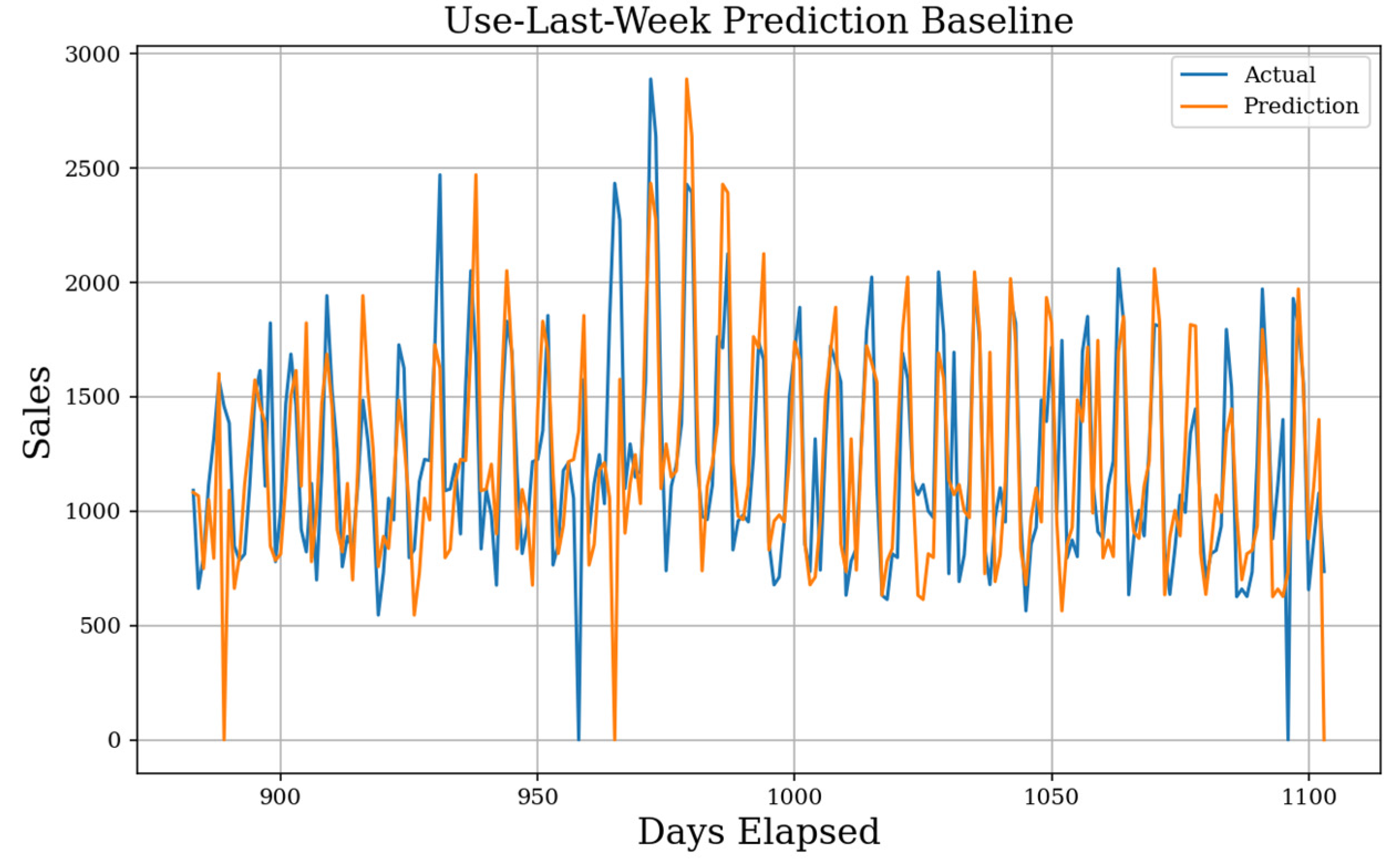
Figure 11.
Enhanced Use-Last-Week Actual Prediction. Using the weekly seasonality and the mean weekday average, the final prediction baseline implements a simple history. The MAE baseline generated is 239, the sMAPE is 21.5%, and the gMAE is 150.
Figure 11.
Enhanced Use-Last-Week Actual Prediction. Using the weekly seasonality and the mean weekday average, the final prediction baseline implements a simple history. The MAE baseline generated is 239, the sMAPE is 21.5%, and the gMAE is 150.
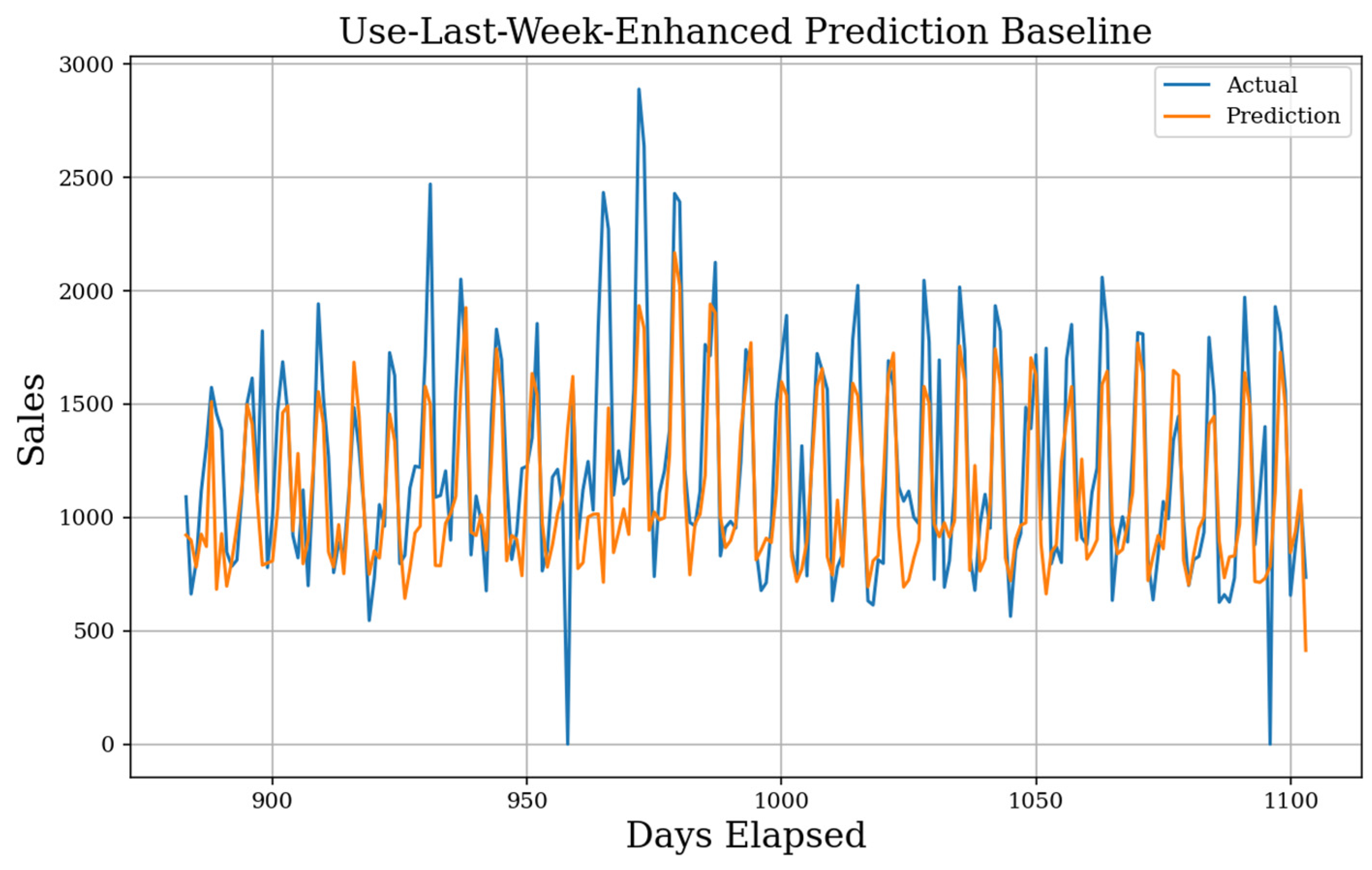
Figure 12.
F-score for Top Features (Actual). The top 25 features as ranked by their F-scores. Weekly sales average is the highest scoring feature by far with other statistical metrics and days of the week following. Numbers 0–13 mark how many days until removal from the prediction window, so temporarily 13 is yesterday, 7 is one week ago, and 0 is two weeks ago.
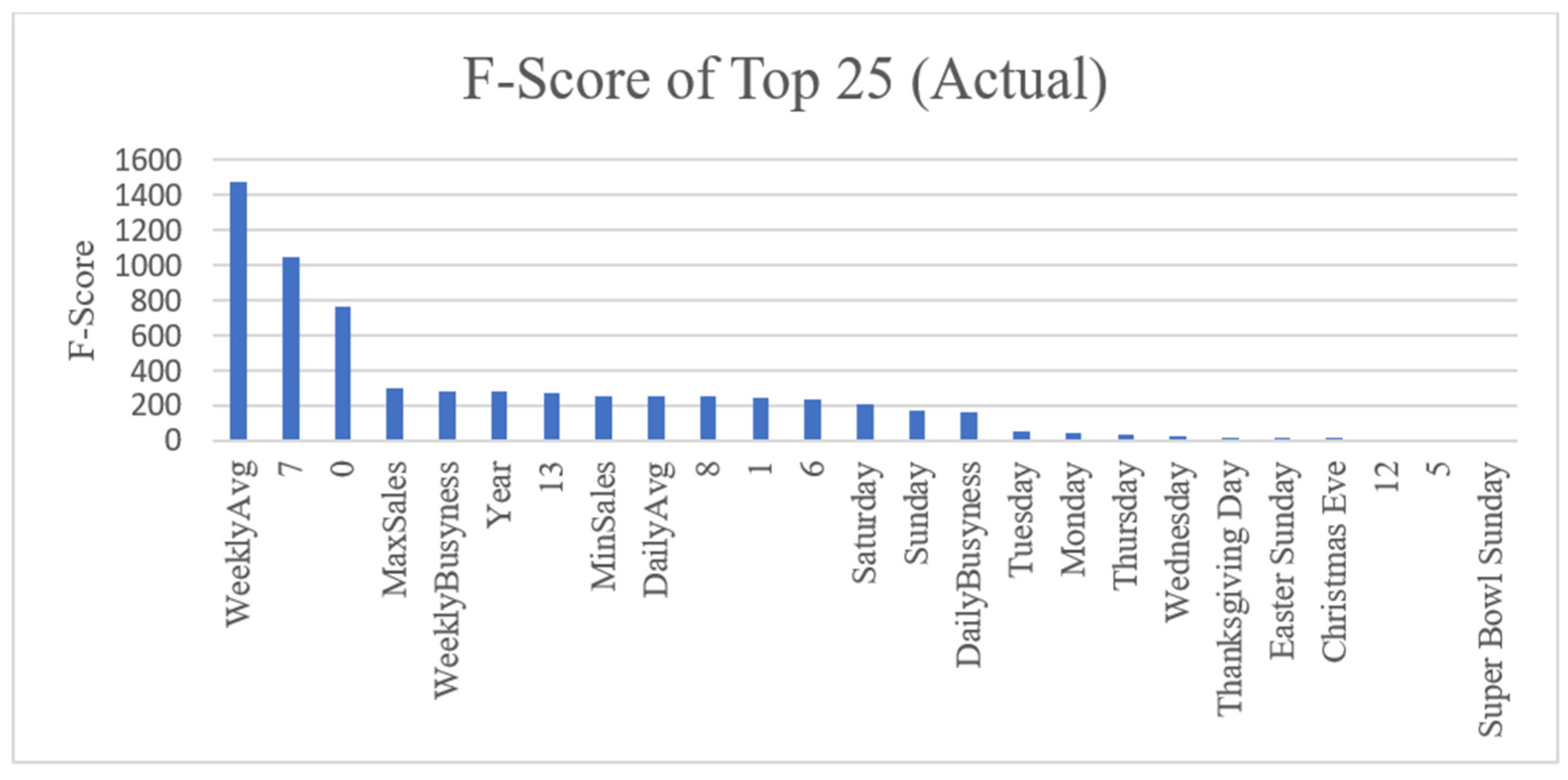
Figure 13.
Best One-Day Forecast MAE Found Across 73 Features (Actual). Recurrent (orange) and non-recurrent (blue) models are trained with an iteratively increasing number of ranked features, seen in Supplementary Materials Figure S10, for one-day forecasting. The lowest MAE for each model is recorded with the number of features next to the model’s name.

Figure 14.
All RNN Models and Ridge One-Day Forecast MAE Across 73 Features (Actual). We show how the number of features affects the MAE score for one-day forecasting in the actual dataset.
Figure 14.
All RNN Models and Ridge One-Day Forecast MAE Across 73 Features (Actual). We show how the number of features affects the MAE score for one-day forecasting in the actual dataset.

Figure 15.
Kernel Ridge Daily Differenced One-Day Forecast. MAE of 214, sMAPE of 19.6%, and gMAE of 126, with 72 features. Original predictions (top) and the transformed back version (bottom) are both shown. This shows the best performing one-day forecast.
Figure 15.
Kernel Ridge Daily Differenced One-Day Forecast. MAE of 214, sMAPE of 19.6%, and gMAE of 126, with 72 features. Original predictions (top) and the transformed back version (bottom) are both shown. This shows the best performing one-day forecast.
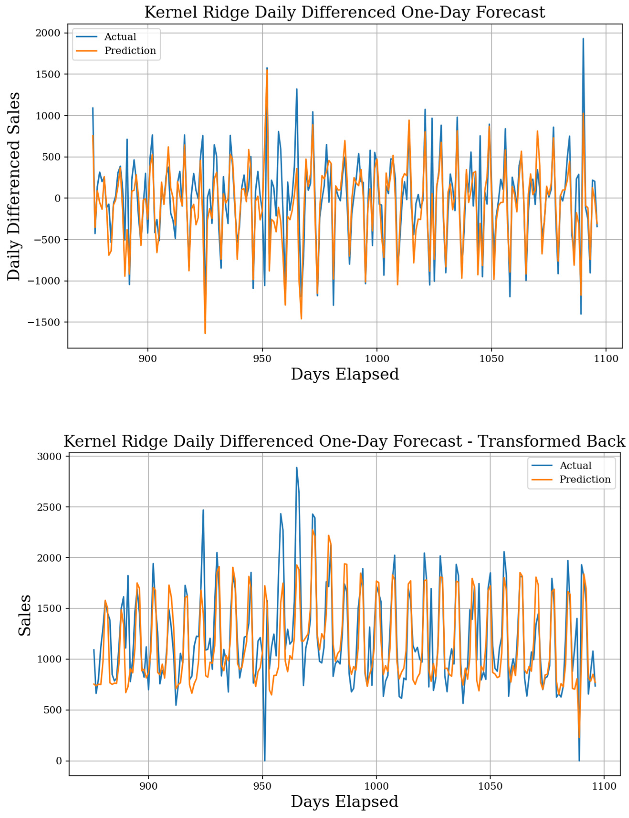
Figure 16.
Transformer Less Features Actual One-Week Forecast. The best start day MAE of 216 is found when starting on Tuesday. A sMAPE of 20.2% and gMAE of 123 show we may look for more improvements in the future, as results are not as good overall as one-day. A mean MAE of 218 and a standard deviation of 1.29 are found with 17 features. TFT perfectly captures the two holiday zero-sale days without acknowledging the zero-sale ‘hurricane day’.


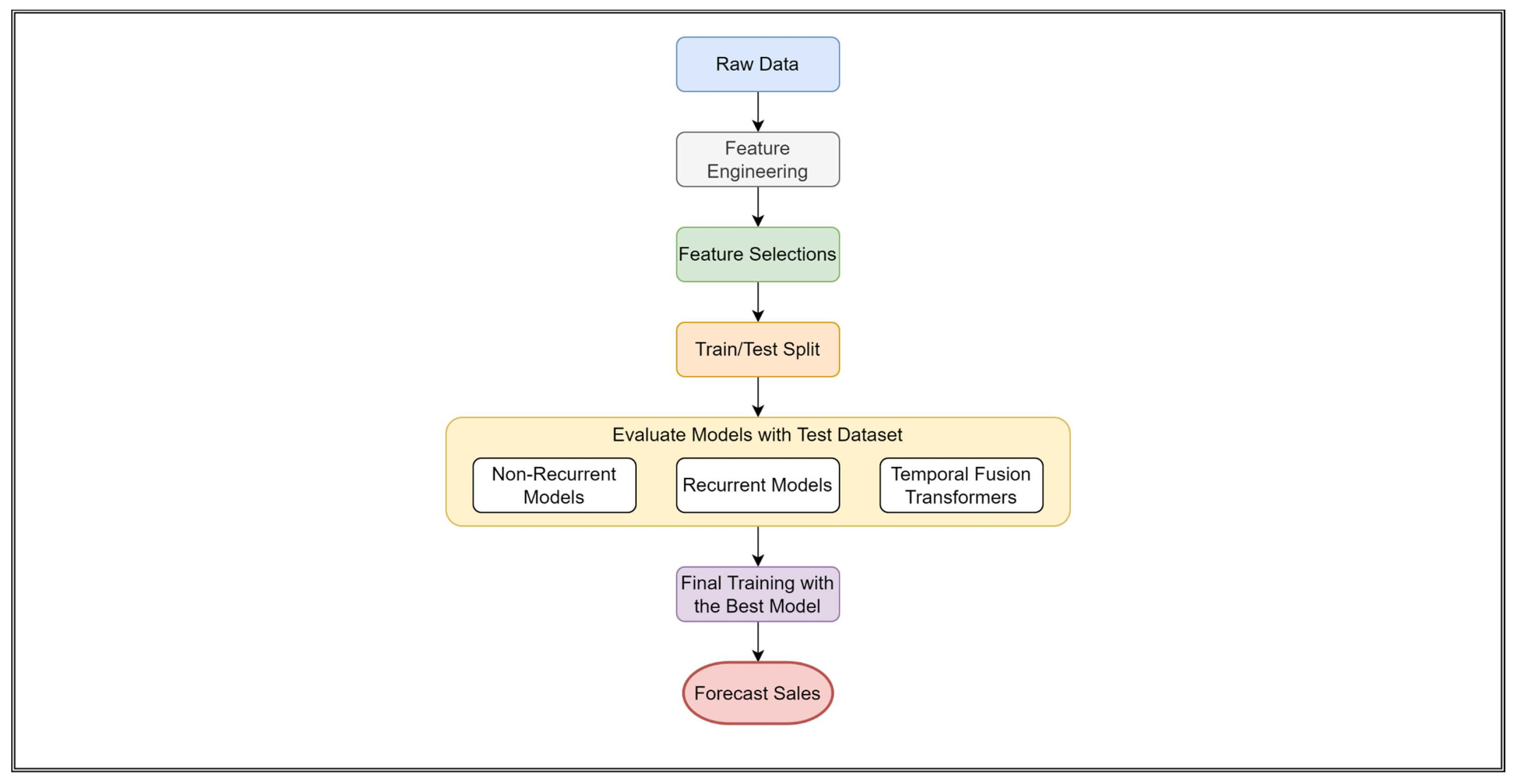
Table 1.
We display each feature used for prediction and a description of that feature.
| Feature Name | Description |
|---|---|
| Year | The year ranging from 2016–2019. |
| Day | The day of the month. |
| Month | Each month of the year. One-hot encoding applied. |
| Weekday | Each day of a seven-day week. One-hot encoding applied. |
| Holiday | 29 different holidays included. Full list can be seen in Supplementary Materials Table S1. One-hot encoding applied. |
| Carnival Season | Mardi Gras holiday season. Lasts from January 6th to Mardi Gras Day. |
| Lent Fasting | Starts Ash Wednesday and end 40 days later. Fasting stops on Sundays and St. Patrick’s Day. |
| Ramadan | One month of fasting. Variable start dates. |
| Christmas Season | 1 December to 25 December. |
| Previous 14 Days of Sales | Each sales or differenced value from the previous 14 days are included as individual features. 14 is chosen as the lookback time, but any multiple of seven would be appropriate. |
| Weekday Average | The weekday average is found as where t is the current time-period and n is the number of preceding weeks. D refers to the set of individual weekdays (ex. All Mondays or all Tuesdays). |
| Daily Average | The day average is found as where t is the current time-period and n is the total number of preceding days. |
| Daily Maximum | |
| Daily Minimum | |
| Predicted Weekday Busyness | where the weekday influences the predicted busyness. |
| Predicted Daily Busyness | where the total average influences the predicted busyness. |
| Daily Differenced Average | See Daily Average, but the daily differenced sales are used. Not included when predicting actual sales. |
| Weekly Differenced Average | See Weekday Average, but the daily differenced sales are used. Not included when predicting actual sales. |
| Minimum Daily Difference | See Daily Minimum, but the daily differenced sales are used. Not included when predicting actual sales. |
| Minimum Daily Difference | See Daily Maximum, but the daily differenced sales are used. Not included when predicting actual sales. |
Table 2.
We display each model used in the case study. The model is given first, followed by which family grouping the model fits in. Relevant resources are listed for further reading and formulae.
Table 2.
We display each model used in the case study. The model is given first, followed by which family grouping the model fits in. Relevant resources are listed for further reading and formulae.
| Model | Family | Resources |
|---|---|---|
| Linear Regression | Linear Models | [24,25,26] |
| SGD Regression | Linear Models | [27] |
| Ridge Regression | Linear Models | [24,25,28,29] |
| Lasso Regression | Linear Models | [26,29] |
| Elastic-Net Regression | Linear Models | [29,30] |
| Bayesian Ridge Regression | Linear Models | [28,31,32] |
| Kernel Ridge Regression | Linear Models | [33,34] |
| Decision Tree Regression | Decision Tree Models | [35,36,37] |
| Support Vector Regression | Support Vector Models | [33,38,39,40] |
| Nu Support Vector Regression | Support Vector Models | [39,40] |
| Linear SVR | Support Vector Models | [41] |
| K-Neighbors Regression | Clustering Models | [42,43,44] |
| Gaussian Process Regression | Gaussian Models | [45,46] |
| Stacking Regression | Ensemble Models | [47,48,49,50,51] |
| Supplementary Materials Table S2 | ||
| Voting Regression | Ensemble Models | [47,52] |
| Supplementary Materials Table S3 | ||
| Extra Trees Regression | Decision Tree/Ensemble Models | [53] |
| XGB Regression | Decision Tree/Ensemble Models | [37,53] |
| LGBM Regression | Decision Tree/Ensemble Models | [37,54] |
| Multi-Layer Perceptron | Neural Networks | [6,54,55,56,57] |
| Recurrent Neural Network | Recurrent Neural Networks | [6,13,58,59] |
| Supplementary Materials Figure S1 | ||
| Long-Short Term Memory | Recurrent Neural Networks | [9,12,13,58,60] |
| Supplementary Materials Figure S2 | ||
| Gated Recurrent Unit | Recurrent Neural Networks | [12,61,62] |
| Supplementary Materials Figures S3 and S4 | ||
| Temporal Fusion Transformer | Recurrent Neural Networks | [5,7,12] |
| Supplementary Materials Figure S5 and Table S4 | ||
| Multioutput Regression | Wrapper Model | [5,63] |
Table 3.
Top 25 One-Day Forecast Results. We show the top 25 results for one-day forecasting from all tests, sorted by dataset, then ranked from best to worst. The model, test MAE, sMAPE, gMAPE, and the dataset used to achieve the result are all given. Some best and worst results from each dataset and the baseline are highlighted. The table is sorted by MAE then dataset, and the best results are seen in the Actual and Daily datasets.
| Model | Type | MAE | sMAPE | gMAE | Dataset |
|---|---|---|---|---|---|
| Stacking | NR | 220 | 0.195 | 142 | Actual |
| TFT Less Features | R | 220 | 0.196 | 133 | Actual |
| Bayesian Ridge | NR | 221 | 0.195 | 144 | Actual |
| Linear | NR | 221 | 0.195 | 144 | Actual |
| Ridge | NR | 221 | 0.195 | 144 | Actual |
| SGD | NR | 221 | 0.195 | 144 | Actual |
| LSTM | R | 222 | 0.196 | 131 | Actual |
| Lasso | NR | 226 | 0.201 | 147 | Actual |
| GRU | R | 227 | 0.2 | 144 | Actual |
| Extra Trees | NR | 231 | 0.204 | 128 | Actual |
| Use-Last-Week-Enhanced | NR | 239 | 0.215 | 150 | Actual |
| TFT All Features | R | 244 | 0.215 | 159 | Actual |
| Kernel Ridge | NR | 214 | 0.196 | 126 | Daily |
| Ridge | NR | 216 | 0.195 | 144 | Daily |
| Bayesian Ridge | NR | 217 | 0.196 | 146 | Daily |
| Linear | NR | 219 | 0.198 | 137 | Daily |
| Lasso | NR | 223 | 0.201 | 141 | Daily |
| Stacking | NR | 223 | 0.2 | 148 | Daily |
| XGB | NR | 241 | 0.214 | 152 | Daily |
| Voting | NR | 238 | 0.213 | 144 | Weekly |
| Stacking | NR | 242 | 0.215 | 139 | Weekly |
| Bayesian Ridge | NR | 245 | 0.218 | 142 | Weekly |
| Kernel Ridge | NR | 245 | 0.219 | 144 | Weekly |
| Linear Regression | NR | 245 | 0.217 | 140 | Weekly |
| Lasso | NR | 246 | 0.218 | 141 | Weekly |
Table 4.
Top 25 One-Week Forecast Results. We show the top 25 results for one-week forecasting from all tests, sorted by dataset, then ranked from best to worst. The model, test MAE, sMAPE, gMAPE, and the dataset used to achieve the result are given. One-week specific metrics such as best start day, the mean of each weekday start, and the standard deviation between each start are also included. Best results are bolded. RNN models with the Actual dataset are the only results to beat the baseline Use-Last-Week-Enhanced. Alternate methodologies for extending non-RNN models to longer horizon windows must be explored further and sorted by MAE then dataset.
| Model | Type | MAE | sMAPE | gMAE | Dataset | Weekday | Mean | Std Dev |
|---|---|---|---|---|---|---|---|---|
| TFT Less Features | R | 215 | 0.202 | 123 | Actual | Friday | 222 | 3.363 |
| GRU | R | 218 | 0.195 | 116 | Actual | Sunday | 233 | 13.477 |
| LSTM | R | 222 | 0.197 | 134 | Actual | Thursday | 228 | 5.339 |
| Use-Last-Week-Enhanced | NR | 230 | 0.203 | 139 | Actual | Tuesday | 232 | 2.437 |
| GRU+ | R | 233 | 0.204 | 136 | Actual | Wednesday | 246 | 14.612 |
| ExtraTrees | NR | 235 | 0.206 | 145 | Actual | Wednesday | 240 | 4.085 |
| Stacking | NR | 237 | 0.208 | 146 | Actual | Tuesday | 243 | 4.634 |
| Voting | NR | 237 | 0.209 | 140 | Actual | Friday | 246 | 8.256 |
| Kernel Ridge | NR | 239 | 0.213 | 143 | Actual | Wednesday | 244 | 4.229 |
| SGD | NR | 240 | 0.214 | 140 | Actual | Tuesday | 249 | 7.712 |
| Bayesian Ridge | NR | 242 | 0.216 | 145 | Actual | Wednesday | 248 | 3.408 |
| Lasso | NR | 243 | 0.218 | 147 | Actual | Thursday | 248 | 2.979 |
| Transformer | R | 267 | 0.239 | 153 | Actual | Wednesday | 268 | 1.131 |
| Lasso | NR | 280 | 1.016 | 162 | Daily | Sunday | 287 | 6.53 |
| Lasso | NR | 253 | 1.284 | 137 | Weekly | Sunday | 256 | 3.156 |
| Ridge | NR | 256 | 1.274 | 144 | Weekly | Sunday | 261 | 3.403 |
| Kernel Ridge | NR | 257 | 1.274 | 146 | Weekly | Sunday | 262 | 3.436 |
| Elastic | NR | 257 | 1.327 | 153 | Weekly | Sunday | 259 | 1.495 |
| SGD | NR | 257 | 1.28 | 148 | Weekly | Monday | 261 | 2.978 |
| LinSVR | NR | 258 | 1.405 | 149 | Weekly | Sunday | 260 | 1.939 |
| Bayesian Ridge | NR | 259 | 1.304 | 151 | Weekly | Sunday | 260 | 1.21 |
| Stacking | NR | 260 | 1.281 | 151 | Weekly | Monday | 264 | 2.694 |
| Transformer | R | 263 | 1.371 | 147 | Weekly | Tuesday | 278 | 9.849 |
| RNN | R | 273 | 1.722 | 162 | Weekly | Sunday | 278 | 2.95 |
| GRU | R | 273 | 1.674 | 154 | Weekly | Sunday | 279 | 4.318 |
Publisher’s Note: MDPI stays neutral with regard to jurisdictional claims in published maps and institutional affiliations. |
© 2022 by the authors. Licensee MDPI, Basel, Switzerland. This article is an open access article distributed under the terms and conditions of the Creative Commons Attribution (CC BY) license (https://creativecommons.org/licenses/by/4.0/).
Share and Cite
MDPI and ACS Style
Schmidt, A.; Kabir, M.W.U.; Hoque, M.T. Machine Learning Based Restaurant Sales Forecasting. Mach. Learn. Knowl. Extr. 2022, 4, 105-130. https://doi.org/10.3390/make4010006
AMA Style
Schmidt A, Kabir MWU, Hoque MT. Machine Learning Based Restaurant Sales Forecasting. Machine Learning and Knowledge Extraction. 2022; 4(1):105-130. https://doi.org/10.3390/make4010006
Chicago/Turabian StyleSchmidt, Austin, Md Wasi Ul Kabir, and Md Tamjidul Hoque. 2022. "Machine Learning Based Restaurant Sales Forecasting" Machine Learning and Knowledge Extraction 4, no. 1: 105-130. https://doi.org/10.3390/make4010006