
Robust Reinforcement Learning: A Review of Foundations and Recent Advances
by
 , ,
, ,
Janosch Moos
1,*,† ,
,
Kay Hansel
2,*,†,
Hany Abdulsamad
2,
Svenja Stark
2,
Debora Clever
1,3 and
Jan Peters
2 1
Institute for Mechatronic Systems in Mechanical Engineering, Technical University of Darmstadt, 64287 Darmstadt, Germany
2
Intelligent Autonomous Systems in Computer Science, Technical University of Darmstadt, 64289 Darmstadt, Germany
3
ABB AG, 68309 Mannheim, Germany
*
Authors to whom correspondence should be addressed.
†
These authors contributed equally to this work.
Mach. Learn. Knowl. Extr. 2022, 4(1), 276-315; https://doi.org/10.3390/make4010013
Submission received: 30 December 2021
/
Revised: 7 March 2022
/
Accepted: 16 March 2022
/
Published: 19 March 2022
(This article belongs to the Special Issue Advances in Reinforcement Learning)
Abstract
:Reinforcement learning (RL) has become a highly successful framework for learning in Markov decision processes (MDP). Due to the adoption of RL in realistic and complex environments, solution robustness becomes an increasingly important aspect of RL deployment. Nevertheless, current RL algorithms struggle with robustness to uncertainty, disturbances, or structural changes in the environment. We survey the literature on robust approaches to reinforcement learning and categorize these methods in four different ways: (i) Transition robust designs account for uncertainties in the system dynamics by manipulating the transition probabilities between states; (ii) Disturbance robust designs leverage external forces to model uncertainty in the system behavior; (iii) Action robust designs redirect transitions of the system by corrupting an agent’s output; (iv) Observation robust designs exploit or distort the perceived system state of the policy. Each of these robust designs alters a different aspect of the MDP. Additionally, we address the connection of robustness to the risk-based and entropy-regularized RL formulations. The resulting survey covers all fundamental concepts underlying the approaches to robust reinforcement learning and their recent advances.
1. Introduction
In recent years RL research has started shifting towards deployment on realistic problems. In an effort to mimic human learning behavior, RL utilizes trial and error-based designs contrary to traditional control designs [1,2]. In control, the optimal behavior is derived from analytical reasoning of physical constraints [1,3,4,5,6]. Such designs are known as white-box models. RL, on the other hand, assumes a black-box approach where the system is unknown. The agent continuously observe the system’s response through interactions. The observed data drives the optimization of the agent’s behavior to achieve a given objective [1,2]. However, the solutions to standard RL methods are not inherently robust to uncertainties, perturbations, or structural changes in the environment, phenomena that are frequently observed in real-world settings.
Definition 1.
Robustness—in the scope considered in this survey—refers to the ability to cope with variations or uncertainty of one’s environment. In the context of reinforcement learning and control, robustness is pursued w.r.t. specific uncertainties in system dynamics, e.g., varying physical parameters.
For example, a common manifestation of this phenomena is encountered when evaluating policies trained in simulation on the real environment. Even for advanced simulators, the deviations between environments gives rise to the sim-to-real gap. This gap leads to a significant drop in real-world performance. Still, the high cost of real physical interactions incentives training in simulation. However, a simulation rarely captures all physical aspects of the real system. Therefore, the transition between simulation and reality entails a high risk of performance loss [7,8,9,10,11].
Robustness has been studied extensively in optimization and optimal control [12,13,14]. Robust optimization adopts a nested optimization architecture [13,15,16]. The inner problem is governed by a set of uncertain problem parameters known as uncertainty set. The outer problem provides optimal solutions robust to all variations within this uncertainty set. However, the nesting architecture leads to conservative solutions and consequently corresponds to worst-case design. Optimal control—a practical application of optimization—also utilizes this architecture for robustness. In optimal control, the system dynamics are described through differential equations [4,5,17]. As in simulations, these equations can only approximate the real system behavior. With increasing complexity of modern systems, determining close approximations becomes challenging [4,5,17]. A well-known approach in robust optimal control is -control [18,19,20,21,22]. Robustness is achieved by describing approximation errors or parameter changes in the environment as disturbances. The system’s sensitivity to its maximum disturbances is then minimized. Robust RL has drawn inspiration not only from robust optimization but also from -control [7,23,24,25].
Formulations based on robust optimization are closely related to game theory. In two-player zero-sum games, a protagonist, i.e., an agent or controller, minimizes an objective function, while an opposing player maximizes the same objective. This competitive framework known as a mini-max game corresponds to the worst-case design. The relation of -control to mini-max games was shown through a linear quadratic formulation of the differential game [26,27,28,29]. Generalized, differential games extend optimal control to multiplayer environments [30,31]. In the single-player case, this framework reverts back to classical optimal control [32]. As such, differential games provide a game-theoretic view of optimal control. Solutions to games are equilibria between the participating players [33]. This concept is a foundation of convergence guarantees in robust designs.
RL leverages the mini-max game to introduce the adversarial reinforcement learning framework. This two-player zero-sum formulation represents a special case of multi-agent reinforcement learning (MARL) in fully competitive environments [34,35,36]. Most research focuses on the deployment of RL in competitive games instead of robustness. The framework, however, is also valid for robust RL. The core difference is the formulation of the opposing player, the adversary. Controlling uncertainty and disturbances through the adversary produces robust protagonists [9,37].
Robustness is constrained to the variations of the inner optimization problem. As such, the adversary’s domain becomes the dictating factor in robust RL. Each robust RL approach targets a different aspect of the MDP. We survey the literature on robust RL and categorize the approaches in four different ways, as follows. (i) RL classically describes the system dynamics as a deterministic or stochastic transition function [1]. Generally, this function is assumed invariant during training. Methods following the transition robust design consider uncertainties in the function itself. Therefore, the uncertainties are modeled as an uncertainty set. An adversary taking control of this set simulates uncertain dynamics [23,24,25,38,39,40,41,42,43,44,45,46,47,48,49,50,51,52,53,54]. Modeling uncertainty in the dynamics directly is a natural choice. However, transition robust design imposes a set of specific assumptions and constraints to remain tractable. (ii) Uncertainties in the system dynamics are equally expressible as disturbing forces—an inspiration taken from optimal control. Disturbance robust design adopts this perspective to formulate perturbing adversaries. These adversaries apply external forces as a source for uncertainty in the system dynamics [7,8,9]. (iii) Action robust design, instead, implies disturbances as perturbations of the agent’s actions. The opposing policies are modeled as part of a joint policy that governs the decision-making process [11,55,56,57]. The joint action is the linear interpolation of the opposing decisions. The mixing parameter regulates the strength of the adversary. (iv) Observation robust design exploits the susceptibility of neural networks to input perturbations. The recent developments inspire these methods in image-based deep learning [58,59]. The adversary leverages the vulnerability to distort the protagonist’s perception. As a consequence, the decision-making process is redirected to a worst-case transition [60,61,62,63,64,65]. The protagonist perceives the shift in transitions as changing dynamics. Hence, transition and disturbance robust designs target elements around the environment. Contrary, action and observation robust designs aim for elements surrounding the decision-making process. Aside from direct robust formulations, we discuss literature on the connection of robustness to risk-based and entropy-regularized RL formulations. Mathematical proofs show the equivalence of certain risk-based and entropy-regularized RL formulations to transition robust designs [66,67,68,69].
First, we discuss the basics of optimization, optimal control, and reinforcement learning. We clarify how these research fields connect and relate with each other. Further, the extension to multi-agent environments and MARL is explained. We present our understanding of robust reinforcement learning separated into the four aforementioned categories. We discuss several extensions and concepts proposed in each category over the past two decades. As most research has been presented in the context of transition robust design, this part is significantly larger than the other categories. Finally, we shortly introduce the connections of robustness to risk-based and entropy-regularized formulations. This survey centers around the core ideas and mathematical framework behind each approach. We cover a large research body of both reinforcement learning and control theory. As such, notations of both topics can be found in this paper. In Table 1, the similarities in the notations we used are clarified. Not all work in robustness is covered in this survey. However, our goal is to provide new aspiring researchers with a solid foundation on robust RL, detailing the fundamental idea behind the four categories and their possible extensions.
2. Preliminaries
The concepts behind robust reinforcement learning are not unique to RL—rather, they are multidisciplinary. Closely related research areas are optimization, optimal control, and game theory. Ideas and concepts from these areas have been repurposed and built upon. This chapter summarizes the fundamentals, i.e., optimization, optimal control, and reinforcement learning. The relations to each other and to game theory are highlighted. We aim to provide a better understanding of the core ideas and their interdisciplinary application.
2.1. Optimization
Optimization provides mathematical tools for solving problems in various areas, e.g., control theory, decision theory, and finance [70,71,72]. In general, an objective function is optimized by finding the correct design parameters . Typically, the domain X represents a subset of a Euclidean space [71]. The problem is formulated as
where the vectors and represent equality and inequality constraints, respectively. In reality, however, the optimization problem must often deal with uncertainties and perturbations [16,73]. Possible causes can be changes in environmental parameters, e.g., angle, temperature, or material. Furthermore, the optimization must be able to handle measurement and approximation errors due to the approximation of real physical systems [73].
Robust optimization approaches tackle these issues by considering a deterministic uncertainty model [13,14,15,16,74,75]. The general assumption considers an extended objective with an additional vector of uncertain problem parameters . This objective is commonly known as robust counterpart. The vector belongs to a given uncertainty set and is not exactly specified. As such, the optimization problem
is extended to a bi-level optimization problem. A bi-level problem corresponds to a game, where a protagonist tries to minimize the objective . Meanwhile an adversary controls to achieve the worst possible outcome for the protagonist. The approach, however, does not consider the benefits of any available distributional information on the problem. Thus, the outcome of the worst-case scenario in Equation (2) is too conservative [73,75].
Stochastic optimization (SO) takes advantage of such distributional information. In comparison to Equation (2), SO treats not as a vector from an uncertainty set. Rather, is a random variable drawn from a known distribution [70,72,73]. The objective is reformulated as
where the protagonist seeks to minimize the expectation of uncertain parameters. SO captures a less conservative risk attitude of the outcome than robust optimization given a stochastic domain. While risk—exposure to uncertain outcomes of a known probability distribution—is captured in both approaches, neither address ambiguity, i.e., the probability distribution itself is subject to uncertainty [75,76].
The distributional robust optimization [77] aims to handle both situations. The approach keeps the potentially uncertain probability distribution in a known set of distributions [74,75]. Due to the a priori known , the distributionally robust optimization problem is formalized as
which again results in a bi-level optimization problem similar to robust optimization. In this scenario, however, an adversary chooses the worst possible distribution . This way, the distributionally robust counterpart captures not only the decision maker’s risk attitude but also an aversion towards ambiguity [75].
The basic concept for optimization see Equation (1) is a core part of optimal control and reinforcement learning. Both aim to optimize a payoff function, which is defined by the underlying environment surrounding the controller or agent. Robust approaches in RL further utilize the concept of robust optimization see Equation (2) or distributional robust optimization see Equation (4)—either directly or from a game-theoretic point of view.
2.2. Optimal Control
Optimal control is a practical application of optimization for dynamic (variational) systems. Such optimization problems are generalized in the calculus of variations (CV) formulated as
is an objective or cost function optimized w.r.t. any variable . The problem is constrained by the conditions and on the start- and endpoint, respectively. The Lagrangian describes the cost at each point in time. Works published by Bolza [78], McShane [79], Bliss [80], Cicala [81] turned out to be important foundations for the adaption of CV to optimal control. In more detail, optimal control aims to calculate optimal trajectories by minimizing an objective function under differential constraint equations describing the system dynamics [1]. Thus, the optimal control problem can be written in the form
known as Bolza form. The goal here is to optimize the cost function w.r.t. the control variable . The first-order differential constraints describe the system dynamics given a current state and control . Constraints on the terminal state are given by with final time which is often written as . Optionally, control and state-space constraints are defined as . As in CV, the Lagrange term describes the cost at each point in time while the Mayer term represents the constant cost in the terminal state [71]. This approach of using first-order differential equations became known as the state-space formulation of control [4]. With the maximum principle Pontryagin [82] formulated the Hamiltonian
for optimal control. The Maximum Principle is an approach for solving such non-classical variational problems (see Equation (5)) by transforming the problem into nonlinear subproblems [5]. Pontryagin [82] states that for a minimizing trajectory satisfying the Euler-Lagrange equations there exists a control maximizing the Hamiltonian.
Hamilton-JACOBI-Bellman Equation
In optimal control Bellman [83] introduced an optimal return or value function
to define some performance measure from state and time t to a terminal state under optimal control [5]. The value function—an extension of the Hamilton-Jacobi equation—takes the form of a first-order nonlinear partial differential equation
later known as Hamilton–Jacobi–Bellman equation (HJB) [71,83,84]. The HJB equation was originally presented in the context of dynamic programming (DP). DP solves optimal control discretized w.r.t. states and actions [83]. Due to the discretization, DP becomes infeasible in higher dimensional spaces known as the curse of dimensionality [1,5].
Discretized w.r.t. time the HJB equation is commonly known as Bellman equation (see Equation (14)) and is a fundamental concept of RL (see Section 2.3). The time discretization causes a sequence of states for which Bellman [85] proposed a Markovian framework known as Markov decision process. It represents a discrete stochastic version of the optimal control problem [1,85].
2.2.1. Robust Control
Parallel to dynamic programming [83], Kalman et al. [86] proposed a more control theory-driven approach known as linear quadratic regulator control (LQR). LQR formed the foundation for the linear quadratic Gaussian control (LQG) [86,87,88]. The goal of control theory remains to find a controller that stabilizes a dynamic system. In these systems, robustness against modeling errors, parameter uncertainty, and disturbances in an environment has long been a big challenge. As such, a robust controller stabilizes a system under these uncertainties and disturbances. While optimal control already accounted for disturbances, it is still not robust under modeling errors and parameter uncertainty [12]. Since the 1980s, research tackling robustness became more prominent under the name robust control [5]. During that time, a new form of optimal control called -control emerged, based on sensitivity minimization [18,19,20,21,22]. For this survey, we want to focus on -control as it provides interesting relations to game theory and robust reinforcement learning.
-control generally optimizes finite linear time invariant dynamical systems described by the following linear constant coefficient differential equations
where describes the system state vector and denotes a control vector with a disturbance given in . , and F are real constant matrices. In the Laplace space the relation of system output and control is given as a linear transfer function
Such a linear system can be reshaped to the form depicted in Figure 1a. The dynamics of this system are defined as
where a stable transfer matrix P represents the plant. The vector signal contains noise, disturbances and the reference signal, while includes all controlled signals and tracking errors. The measurement and control signals are represented by and , respectively. The linear transformation is governed by the transformation matrix
Optimal -control is defined as to find all admissible controllers K such that
is minimized, where corresponds to the largest singular value. By definition, a controller is admissible if it internally stabilizes the system [12]. This formulation represents a worst-case design as it minimizes the system’s sensitivity to the worst possible case of disturbances.
Robust stability, however, is only given if a controller K stabilizes the system not only under noise and disturbances but also under parameter perturbation and model uncertainties as depicted by in Figure 1b. According to the small gain theorem, this system is deemed stable for any perturbation in with if the controller ensures that with some [12,27]. Coming from robust optimization, represents a known uncertainty set containing all possible disturbances and parameter perturbations of the nominal plant.
Relations to Game Theory
An important observation is that the -control problem minimizes the maximum norm. Reformulating Equation (9) under the small gain theorem represents a cost function of the form
where depends on and . Using this cost function, an optimal value function is formulated as
As such, -control represents a mini-max optimization problem or a mini-max game. Generally, mini-max games are zero-sum games, where the controller and the disturbances or uncertainties are each represented as one player. While -control is in the frequency domain, robust control in the time domain corresponds to a differential game. Basar and Bernhard [27] show the connection between -control and differential games in more detail in their book.
2.2.2. Differential Games
Game theory has its roots with Von Neumann and Morgenstern [89] defining various types of games, settings, and strategies [31]. The differential game, however, was only later introduced by Isaacs [30]. These differential games provide a unique game-theoretic perspective on optimal control. In general, a differential game is written as a multi-objective optimization problem representing a situation where N players act in the same environment with different goals or objectives. We will refer to these players as agents. The objectives are defined as a payoff [90] or cost function [33] for each agent i, with
Note that the payoffs are written in Bolza form, similar to optimal control (see Equation (5)). The Lagrangian of each agent i depends on the whole set of all agents. Isaacs [90] proposed two kinds of games. The game of kind describes discrete and the game of degree continuous cost functions. The former, in most cases, describes an objective of a yes–no type of possible payoffs, e.g., win or loss of a game.
The system dynamics in a multi-objective optimization problem are written as a first-order differential equation
depending on the world’s state and the agents’ actions [90]. An agent follows either a pure or mixed strategy determining which action to choose from a set of actions the agent is given for each state [90]. Pure strategies are of the exploiting deterministic type. In each state, the agent chooses the best possible action without exploration. Mixed strategies, in contrast, are stochastic and thus also incorporate exploration. The agent maintains a distribution over the given action set for each state and draws samples to determine the next action to execute. An agent playing mixed strategies always wins against an agent playing w.r.t. pure strategies because of its deterministic behavior. In multi-objective optimization, the set of strategies is expressed as
Approaches to solving such a game depend on the available information for each agent. Commonly, each agent is aware of the current value of the state, the system parameters, and the cost function. The strategies of the adversaries, however, are unknown [33]. Another important piece of information is how the agents interact with each other. In game theory, there are different types of games determining the interaction of agents. A cooperative game refers to a situation where a subset of agents acts in unison to reach a mutually beneficial outcome. This setting can be extended to all agents acting in unison to reach a common goal that corresponds to a fully cooperative or team game. Respectively, a non-cooperative game represents a situation without cooperation. Each agent chooses its actions regardless of the cost inflicted to other agents [31,37,89,91,92]. The solutions to these types of games provide a balance between the independent interest of the agents called equilibrium [31,90,91].
2.2.3. Nash Equilibrium
In non-cooperative games, however, convergence to a globally optimal equilibrium is not guaranteed, which instead requires Nash equilibria [91]. In a Nash equilibrium, it is guaranteed that each agent deviating from the equilibrium increases its costs. In turn, agents acting optimally w.r.t. the equilibrium get their costs lowered. A strategy set is a Nash equilibrium if
holds for each objective , where is any admissible strategy for agent i. There are methods utilizing this property, e.g., the value function approach (dynamic programming) or the variational approach (analytic, see calculus of variations) [33]. However, the existence of a Nash equilibrium is not guaranteed for all non-cooperative games.
Another challenge in general non-cooperative games is the lack of information, as agents do not exchange information about their strategies. Hence, the agents cannot be sure that their adversaries act w.r.t the Nash equilibrium. The resulting optimal strategy for an agent might therefore not necessarily follow the Nash equilibrium. An intuitive but excessively pessimistic approach is the assumption that every other agent behaves adversarially. This approach corresponds to a situation where an agent’s cost is maximized by all of its adversaries. An agent thus aims to minimize its maximum cost, the basic idea behind mini-max games. Such problems are defined in the following form
which does not take the payoffs of the other agents into account for agent i [31,33,35,90].
2.2.4. Two-Player Zero-Sum Game
An extreme case is the two-player zero-sum game where two agents play against each other as adversaries such that the objectives are directly opposed
The sum of the objectives of both agents amounts to zero [31,90,91]. As shown in Figure 2, the Nash equilibrium corresponds to a saddle point solution in a two-player zero-sum game. So we can rewrite the Nash equilibrium to become
If this equation holds, there is a Nash equilibrium [27,90,91]. Further, if a Nash equilibrium exists, this equilibrium is equivalent to the solution of a mini-max optimization for two-player games [33]. Additionally, the existence of a Nash equilibrium is guaranteed if mixed strategies are allowed. Therefore, the two-player zero-sum game guarantees the existence of a mini-max solution for mixed strategies [93]. However, this property does not hold for player games.
A special variant of the zero-sum game is the game against nature. It describes a situation in which one agent’s actions correspond to environmental disturbances (nature) that other agents must overcome. Thus, nature and the agents work on completely different action spaces [37]. In terms of optimal control, this situation comes closest to -control as a worst-case design under uncertainties and disturbances. It is also possible to give nature control over the parameters of the environment to incorporate modeling errors and thus more closely represent robust control.
2.3. Reinforcement Learning
Despite the long history of research and success in optimal control, it differs considerably from human control (Table 2). Instead of defining the environment’s behavior mathematically and designing a system from scratch to control said behavior, humans learn to control by repetitively interacting with their environment. This human approach to control is adopted in reinforcement learning. An agent learns to map certain situations or states in an environment to actions while maximizing its short and or long-term reward [1]. Still, reinforcement learning is based on ideas from optimal control. Every action the agent takes has an impact on the environment and, in most cases, causes a change of the environments’ state. Such change in turn is observed and acted upon.
2.3.1. Single Agent Reinforcement Learning
A fundamental concept for the environment was introduced through Bellman’s research with the development of the Markov decision process. A schematic of this mathematical framework describing the interplay of an agent and its environment is shown in Figure 3. A key assumption behind the MDP is the Markovian nature of the system, commonly known as the Markov property. This property states that a fully observed state is statistically sufficient. In a statistically sufficient state, the transition probability can be determined only based on the observation and taken action without knowing the history of previous states, i.e., the transition probability is conditionally independent of the transition history. In the standard formulation, we assume a fully observable MDP where the agent can fully observe the state of the environment at each time step [1,2,9,34,85,94,95,96]. As described in Section 2.2.1, the MDP was designed to tackle a discretized version of the state space formulation of optimal control w.r.t. time [85]. The MDP is defined by the tuple , where all possible states of the environment are represented by . On the other hand, contains all possible actions of the agent, respectively. The system dynamics are described by a deterministic or stochastic transition function mapping each set of state and action to a new state . By this definition, the transition function of a finite state MDP can also be seen as a 3-dimensional matrix containing a probability for each -tuple. For a specific state this matrix reduces to a 2-dimensional matrix. Each row then describes a probability distribution over next states corresponding to a specific action as defined by
The actions are rewarded by a continuous function . As an example let us assume a system with two possible states , and two possible actions and . Further, we assume to be in state . Then the transition matrix for state can be written as
As many papers in this survey assume a finite state space, we will use the terms transition function and transition matrix interchangeably. The full stochastic dynamics are then defined with a probability function formulated as
In cases where the observed state no longer fully describes the true state of the environment, the observed state loses its property of being statistically sufficient. For example, the observed state may be identical in two different states of the environment. Such scenarios can often occur in real-world applications. To track the true state, the agent must maintain a belief that contains knowledge of past states to estimate which of the true states is represented by the observed state [97,98]. A standard MDP formulation is solved based on statistically sufficient belief states representing this belief. This concept is known as partial observable Markov decision processes (POMDP) [97,98].
In a fully observable MDP setting, reinforcement learning aims to find an optimal deterministic policy . From its origin, the optimal policy formulates an optimal control at each time step, maximizing the expected return of the objective function
where describes the discount factor reducing the influence of future rewards. The horizon T is defined as the maximum time of operation, possibly infinite, or the time required to reach a final or terminal state. In the infinite horizon case, the optimal policy becomes stationary [2].
Converging to an optimal policy , however, is, in theory, only guaranteed if every action is executed infinitely often in each state [1]. A greedy policy exploiting the best action logically is a reasonable choice as it maximizes the known rewards. Nevertheless, there is no guarantee that the known actions are best as some actions might not have been tested yet. Actions that have not been explored have no estimate for their long-term reward and, as a result, will never be chosen. Exploring new actions carries the risk of lowering the short-term reward, but, in turn, the long-term reward may rise eventually. Finding admissible solutions requires a fine trade-off between exploring the unknown and exploiting the known, commonly referred to as exploration vs. exploitation dilemma [1]. A common approach is using a stochastic policy sampling an action from a distribution in a given state . As each action in a state is initially given a probability , exploration is guaranteed. Still, any stochastic policy can converge to a stationary deterministic policy , fully exploiting the system to gain the maximum reward [1,2].
The question remains on how to evaluate each action. Using the immediate reward is possible but contains no information about the future. An action might be attractive for now but leads to a low series of rewards in the future. A common concept most reinforcement methods are based on is the value function or simplified HJB Equation [1,83,85]. Even though the value function cannot be calculated directly, [83] shows that it can be estimated backward from the final to the initial state for the discrete-time setting. Hence, the state-value function V and action-value or Q-function Q are defined as
As the name suggests, the optimal state-value function describes the maximum value one can get from state onwards. In turn, the optimal action-value function represents the maximum value one can get if action is chosen in state .
Bellman [83] introduced the key for a large variety of RL algorithms in the form of dynamic programming for finite space MDPs. Even though dynamic programming was developed in the context of optimal control, one might argue that it is a shared part of the history of optimal control and reinforcement learning [1]. This algorithm breaks down the backward estimation into subproblems. Each subproblem only considers the reward between two consecutive states in a trajectory. The true value function can then be found by recursively solving the subproblems. Thus, a policy will be optimal if it behaves greedy w.r.t. this function [1,2]
This solution requires finite state spaces as it keeps a lookup table for the values in every state. As the lookup table grows exponentially with the number of state variables, each variable introducing a new dimension, dynamic programming carries the risk of the curse of dimensionality. Methods derived from dynamic programming directly using the same table-based formulation are commonly known as tabular methods and suffer from the same problem. The RL community tackled the curse of dimensionality using function approximators [1,99,100,101,102]. Still, as we will see in Section 3.1, dynamic programming is often used as a foundation to show convergence guarantees under different MDP formulations. One concept regularly used in reinforcement learning for optimizing value functions is the temporal difference (TD) Error. The TD Error, described by
is the difference between the current estimate of the value function and a new sample from interacting with the environment. One can optimize the value estimate by minimizing the TD Error. Other common approaches utilize parametric policies instead, where the parameters are updated based on gradient descent w.r.t. the objective (see Equation (11)) [99,103,104,105,106,107,108].
2.3.2. Multi Agent Reinforcement Learning
Reinforcement learning, as we have discussed to this point, assumed a lone agent in a fixed, stationary environment. This secluded view of a learning environment is often unrealistic. Agents often have to interact with other agents in the same environment, and the environment might not be stationary [95]. The crucial assumption of the Markov property is violated through the existence of the other agents as soon as their policies are non-stationary [34,109]. These additional agents cause the environment to become non-stationary and non-Markovian from the perspective of a single traditionally trained agent [110]. A straightforward approach to training these agents in multi-agent environments is called independent learners. Each agent utilizes the simple assumption that no other agents exist or treats them as stationary, causing the environment to be stationary again [93]. For independent learners, the optimal policy is stationary and deterministic, which for standard MDPs is undominated. Undominated means that this policy achieves the highest possible reward from any state amongst all possible policies. This property no longer exists in the case of multiplayer environments as the performance of any policy highly depends on the other player’s choices. A deterministic policy will never be optimal in a multiplayer environment as it is unable to react to other players or opponents and is prone to be exploited [34]. A simple example is rock, paper, scissors. An agent who is deterministic by constantly choosing the same action will always be defeated by his opponent, while an optimal stochastic policy at least breaks even [34]. A more reasonable approach is joint action learners taking information of their opponents into account [111]. As the multi-agent system exhibits the nature of a game-theoretic framework, the Nash equilibrium (see Section 2.2.3) is certainly a possible solution. In this equilibrium, an optimal policy is defined as the best response to all other policies if they act after the equilibrium [34]. Due to the guarantees of the Nash equilibrium in two-player zero-sum games, the adversarial setting is the easiest case of multi-agent reinforcement learning.
The stochastic game, as introduced by Shapley [112], provides an extension of game theory to MDP environments. Hence, the stochastic game or Markov game is a natural extension of the reinforcement learning framework to multi-agent systems [95,113,114]. The Markov game is defined by a tuple with a set of states , and a collection of action sets each . Each set of actions is assigned to a single agent in the environment. The transition function is extended to the form depending on the current state and a chosen action of each agent. This function can again be formulated as a probability . Instead of a single reward function, each agent i is given its own reward function . As before, denotes the discount factor [9,34,36,95]. The state-value function V and Q-function Q are then rewritten from the perspective of agent i as
where [11,34].
The Markov game describes a series of matrix games, where each matrix game or subgame represents a state of the Markov game. In the case of two agents, these subgames are defined by a matrix r where each component contains the instantaneous reward for an action i of agent 1 and action j of agent 2 [95]. This matrix game has to be solved at each stage of the Markov game. As a generalized formulation, the matrix game is defined by a tuple with n players where each player i is given an action set and a payoff function . The payoffs are visualized as an n-dimensional matrix r [93].
These types of games require stochastic policies as any adaptive agent may learn to exploit deterministic behavior as described in Section 2.3.2. In fact, optimal behavior is achieved when the agent is in a Nash equilibrium, where the agent’s policy is the best response to every other policy in the equilibrium. That means any deviation from that policy results in a decrease in reward [34]. Since only two-person zero-sum games guarantee the existence of a Nash equilibrium at every stage of the game, they are the only case with a tractable solution [34,115,116].
For two-player zero-sum cases, the definition of the Markov game can be reduced to a tuple . The collection of action spaces is reduced to for the agent and for its adversary, respectively. Due to the nature of zero-sum games, both agents optimize a single reward function in opposite directions as described in Section 2.2.1 [9,95]. On this basis, the state-value and Q-function are simplified to
where [11]. Since the protagonist maximizes the reward, this definition is equivalent to the generalized form in Equations (16) and (17) when using and . A schematic for this environment is shown in Figure 4.
Littman [95] was one of the first to tackle two-player zero-sum games using reinforcement learning in a multi-agent learning approach. He proposed a new variant of Q-learning, which, in the standard form, tries to approximate the Q-function. This approximation minimizes the error between the Q estimate in the current state and the observed reward plus the Q estimate of the following state. Instead of a maximum Q estimate depending only on a single agent, he proposed a mini-max update depending on the maximizing action of one agent and the minimizing action of its opponent [95]. His training environment was designed as a two-player soccer game with a rectangular position grid. Littman [95] tested four different scenarios. Two agents were trained using standard Q-learning (independent learner) and two using mini-max Q-learning (joint action learner). In both cases, one agent was trained with an opponent choosing random actions and one with an identical copy of himself. All trained agents performed well in a test match against an opponent choosing random actions. However, the results showed that the joint action learner trained against a random opponent performed worse than the independent learner counterpart. Since the independent learner was not taken advantage of by the purely random opponent, its optimization was more effective compared to the joint action learners’ optimization having an optimal opponent in mind. In another experiment, Littman kept the trained independent, and joint action learners fixed to train a new challenger for each of the four agents. Unsurprisingly the result changed dramatically, with both independent learners not winning a single game while the joint action learners still won ∼35% of the games. The joint action learner, who was trained against itself, performed better than the one against a random opponent [95].
Uther and Veloso [35] picked up on Littman’s work to further investigate multi-agent reinforcement learning techniques in a two-player zero-sum setting they described as an adversarial environment. Their work introduced the term of adversarial reinforcement learning as a special variant of MARL. One insight of their work is the big disadvantage of mini-max Q-learning assuming an optimal opponent, i.e., pessimistic behavior. They proposed incorporating a modeled probability distribution over the opponent’s actions in each state to take advantage of an opponent’s suboptimal behavior [35]. However, a huge problem of tabular methods like Q-learning that maintain a table of Q values for each state–action pair is the massive explosion of possible states with increasing numbers of agents. Uther and Veloso [35] discussed two solutions for this problem. The first generalizes over similar states using function approximators, effectively reducing the number of samples required to have an estimate for each possible state. The second solution is watching the opponent to gather more samples from the same amount of moves to converge more quickly to good estimates of the Q values in the table [35].
These approaches presented in [34,35,95] boost the performance of reinforcement learning in two-player games compared to independent learning approaches, but they do not tackle a central issue of reinforcement learning—robustness. Still, they are major milestones for significant contributions to the research of solving two-player games and beyond [117,118,119,120,121,122,123,124,125,126]. It is known from robust optimization and robust control that the two-player zero-sum game equivalent to a mini-max formulation can be used to gain robustness against parameter perturbations and modeling errors. The question here is how the adversary must be designed to gain robustness against specific environmental variations. This topic will thoroughly be discussed in the following chapter.
3. Robustness in Reinforcement Learning
Despite the success and attention classic reinforcement learning has received over the last years, it often struggles with robustness and generalization. This problem is mainly caused by agents overfitting to the specific training environment, which is a major challenge at deployment time. Training of reinforcement learning agents is often done in simulation due to the high cost of interaction with physical systems. In turn, the simulation is an imperfect representation of reality containing modelling errors and imprecise parameters. The difference between simulation and reality is often too large to handle for the trained policy during transition. Even policies trained on the real system directly do not perform well under previously unencountered uncertainties or disturbances. Even slight deviations in the environment’s parameters e.g., mass or friction can have significant impact on a policies’ performance. Such changes are a common occurrence in test scenarios and can be the difference between success and failure [7,8,9]. As shown in Section 2.2 it is possible to leverage the idea of two-player zero-sum games or mini-max solutions to gain robustness to disturbances and environmental parameter variations. Further, Xu and Mannor [127] show that supervised learning algorithms robust to noise and disturbances also provide desirable generalization properties. Even though, it is not clear how this proof holds in reinforcement learning, it is believed that there is a similar connection [11].
Our main interest lies in the robustness of reinforcement learning to parameter variations of the environment. Considering the fundamental definition of the MDP as a tuple , there are multiple options available where additional uncertainty can be placed. Any change in the environment’s states is a reaction to the agent’s actions described by the transition function . Thus, arguably the most intuitive choice is robustness to uncertainty in the transition function such that not only the transitions are uncertain but also the function itself is subject to uncertainty. Based on the concept of robust optimization, introducing an uncertainty set over transition functions , one can formulate a robust MDP [23,24,25]. As robust optimization is defined as a mini-max optimization, the uncertainty set can be seen as an action space for an adversary in a two-player zero-sum game. The adversary is governing the system’s dynamics in the form of the transition function [128]. A similar formulation has also been presented for uncertainty in the reward function [23,24,25].
While intuitive from the perspective of the MDP formulation, uncertainty in the transition function is not the only way to achieve robustness against environmental parameter variations and disturbances. Another approach leverages the idea of robust control by formulating parameter uncertainty as disturbances in the environment represented by an adversary. This adversary would then apply forces to the protagonists body to simulate changes e.g. in mass, gravity or friction [7,8,9].
Similar to how disturbances can describe a change in certain environmental parameters such as friction, a change in these parameters can also describe a disturbance. A common ground between disturbances and parameter variations is that both cause a change in the environment’s behavior. The agent can no longer rely on the transition probabilities being fixed for any given state–action pair. During our research, we identified a similarity in all approaches to robustness against changing system dynamics caused by parameter uncertainty, disturbances, and modeling errors. The key component the different approaches aim for is variability in the transition probabilities. As such, an adversary can also be designed to manipulate the protagonists actions directly. Manipulating the actions alters the transition probabilities from the perspective of the originally chosen action. The agent perceives this alteration as an unexpected, possibly undesirable transition between states [11,55,56].
The same effect is achieved by manipulating the protagonist’s observation of states. By tricking the protagonist into wrong beliefs about the environment’s current state, the protagonist maneuvers itself into unexpected worst case situations [62,63,129].
Over the last years, promising results to parameter robustness have been published using these four basic approaches. We will discuss the different ideas in detail in this section, including some of their variations presented over the years. We try to show how the approaches connect to the basic concepts introduced in the previous section and other related research to the best of our understanding.
3.1. Transition and Reward Robust Designs
Given the underlying stochastic nature of an MDP, every interaction between agent and environment causes a shift in the environment’s state. This change is governed by the transition probability model . A consequence of this stochastic process is the risk of potentially encountering critical states. To minimize this risk in traditional RL, Heger [76] adopted a two-player framework similar to Littman [95]. In Heger [76], however, the adversary takes control over and hence is modeled in the environment. This framework provides a guaranteed minimum performance by considering transitions with the worst outcome at each time step. As a result, the optimal agent behaves risk-averse but also very conservatively [23]. However, this approach abandons the underlying stochastic properties of the environment, replacing the stochastic nature with a deterministic worst-case design [23]. Further, Heger [76] does not seek robustness w.r.t. to errors in the approximation, disturbances, or other outside influences. Instead, the goal should be to derive optimization approaches that are robust against these external uncertainties while also retaining the underlying stochastic nature of the environment. As such, robust reinforcement learning rather considers a layered approach of robust stochastic optimization. This consideration first gained attention in the 1970s where it was applied in Markov decision processes with imprecisely known transition probabilities (MDPIP) [23,128,130,131]. The unknown transition matrix is assumed to be fixed and lies within a known uncertainty set of possible transition matrices . In the case of an infinite horizon with discrete finite state and action spaces, the MDPIP framework can be formulated as a zero-sum stochastic game between protagonist and adversary [112]. Thus, compared to [76], the goal is then changed to optimizing over the worst possible transition matrix instead of a single worst-case transition, a mini-max problem of the form
In this formulation, optimization over is still a deterministic process, but the optimization over remains stochastic as each is a stochastic transition matrix. In general, however, it is NP-hard to find an optimal memoryless policy for Equation (18) with brute force [132]. In contrast to a two-player simultaneous game in which both agents interact simultaneously, the protagonist first tries to maximize the expected return. Then, based on the protagonist’s action, the adversary selects the worst possible transition matrix within an uncertainty set . The interaction of this two-player game is shown in Figure 5. Intuitively, due to this additional information, the behavior of an optimal policy for the adversary becomes static. Each time the adversary encounters the -pair, it will select the same transition matrix out of . Thus, it is also possible to find an optimal stationary policy for the protagonist, which behaves deterministically [128,130]. Nevertheless, finding a solution for statically behaving adversaries is computationally expensive.
Therefore, Bagnell et al. [23] considered a two-player zero-sum dynamic game of complete information defined by
as a lower bound for the static game. The gap between the solution of the dynamic game Equation (19) and the static game Equation (18) goes to zero if the horizon T goes to ∞ [23,24]. In the case of the dynamic game, the adversary’s policy is not restricted to remaining static during the game. The adversary is thus able to explore the uncertainty set to find the worst possible transition matrix for each -pair. Finding a solution for general uncertainty sets, however, is still NP-hard [45].
To improve tractability, Nilim and El Ghaoui [24] and Iyengar [25] have modeled the uncertainty set as a Cartesian product of individual -dependent uncertainty sets
Here, represents the probability simplex for each that describes the uncertainty of state given action [24]. This property (Equation (20)) is known as the -rectangularity property. Intuitively, it permits the adversary to select a transition matrix from without considering transition matrices from other state–action pairs. This property provides the foundation of the robust Markov decision processes (RMDP), defined by a tuple .
Initially, uncertainty sets were constructed based on polytopes or interval matrices [23,128,130,131]. Inspired by game theory, Bagnell et al. [23] have proven that there are optimal stationary deterministic policies both for the protagonist and for the adversary if the uncertainty set is a compact and convex polytope. Therefore, the authors have stated that there has to be a robust value iteration to find optimal policies. However, solving this bi-level optimization problem is computationally expensive [23]. Although these sets can satisfy the -rectangularity property, they are not statistically accurate enough to represent uncertainties [24,25]. For this reason, Nilim and El Ghaoui [24] and Iyengar [25] have constructed uncertainty sets, which are described by likelihood or entropy bounds, which also have a significantly lower computational effort. Using these bounds and an estimated or known reference distribution is a natural way to construct statistically accurate uncertainty sets. Although these sets are not convex, Nilim and El Ghaoui [24] and Iyengar [25] have finally proven that the robust dynamic programming algorithm will find an optimal stationary deterministic policy for all uncertainty sets as long as the -rectangularity property is satisfied. Moreover, given this uncertainty set, the complexity of solving the problem is only slightly higher than for a classical MDP with a fixed transition matrix [24,25].
Subsequently, Wiesemann et al. [45] has presented a generalization of the -rectangular uncertainty set
which is known as -rectangularity. Robust dynamic programming algorithms constraint to this less restrictive property can still find optimal stationary policies. While optimal policies are deterministic in Equation (20), now they may as well be stochastic [45].
A slightly different setting from standard robust MDPs is presented by Lim et al. [44], who aim to solve the robust MDP in the presence of an unknown adversary, meaning that the full extent of nature’s ability to change is unknown. An MDP described by the tuple with finite state and action space is considered. As in standard robust MDPs, a possibly history dependent compact uncertainty set over transition matrices is defined for every state–action pair. However, only a subset of state–action pairs is truly adversarial while all others behave purely stochastically, i.e., with a fixed , as in non-robust MDPs. By optimizing a regret, one can determine a policy as good as the mini-max policy without knowing either or . Such solutions slightly deviate from the common solution to robust MDPs as they are more optimistic and hence indirectly address a major issue of robust approaches based on worst-case analysis.
The worst-case analysis is prone to produce overly conservative policies that achieve only mediocre performance across all possible model parameters in exchange for increasing the worst-case performance [39]. As such, in cases where the nominal model parameters already provide a reasonable representation of the real physical system, a non-robust approach leads to higher-performing policies on that system. In other words, applying worst-case analysis to problems with only a small sim-to-real gap may lead to worse performance. Xu and Mannor [39], therefore, propose a trade-off as a weighted sum between a nominal and a robust performance criterion. In their paper, the authors consider an MDP with an uncertain reward function . The performance criteria are then defined as the expected return at step t for their respective parameters
where is the nominal reward, P is the nominal criterion, and R is the robust criterion. Therefore, the weighted sum is
with being the weighting parameter. A policy is said to be Pareto efficient if it obtains the maximum of among all policies with a certain value of . Xu and Mannor [39] show that this problem can then be solved using parametric linear programming for the whole set of Pareto efficient policies. Unfortunately, this approach only considers uncertainties in the reward function. In the case of uncertain transitions, as presented in [23,24], the authors, Xu and Mannor [39], prove that a solution is not Markovian and, as such, may be intractable. However, the idea of trading-off nominal and robust performance has been adopted for a robust policy optimization algorithm for unknown, noisy system dynamics with possibly noisy observations [52]. The algorithm is based on multi-objective Bayesian optimization, where the objectives represent a nominal performance measure and a robust performance measure , with being the policy parameters. The solution to this optimization problem is defined as a Pareto set that contains all parameters with iff , such that [52]. Their work has shown that the underlying concept of a trade-off between nominal and robust performance is viable for uncertain transition functions.
A different realization of such trade-offs is presented in [41]. The authors propose a chance constraint formulation based on risk assessments for the expected performance of a policy. Assuming that the transition function p and reward function r are drawn from probability distributions and , Delage and Mannor [41] define the chance constraint optimization problem as
which describes the risk-adjusted discounted performance of an uncertain MDP. The constraint in the optimization guarantees with a probability of that the expected performance of will be greater or equal to y given and . For , this problem becomes equivalent to the worst-case analysis of robust MDPs [41]. In this sense, the presented approach relaxes the constraint of worst-case analysis, which is to guarantee minimum performance at all times.
While the trade-off in [39,52] is an intuitive counter to the conservatism of the worst-case analysis, other research targets the rectangularity assumption as the main source of the problem [42,47,48]. The rectangularity assumption is the necessary assumption that the uncertainty in each state is uncoupled from all other states as general coupled uncertainty sets are intractable [42,47,48]. The consensus is that defining tractable uncertainty sets with coupled uncertainty across states mitigates the problem of overly conservative solutions.
Mannor et al. [42] initially proposed the idea of lightning does not strike twice (LDST). The algorithm targets systems where the parameters of transition and reward function deviate from their nominal representations , only in a small number of states . This consideration is made under the assumption that a deviation has a low probability. The total number of states allowed to deviate from their nominal parameters is hence bounded by [42]. Following the example of [24], the authors consider a stationary and a time-variant model for applying LDST. In the stationary model, all deviations from the nominal parameters are chosen at the beginning of an episode and kept fixed thereafter. The resulting optimization problem is defined as
where and refer to state-specific representations of the transition and reward function. Accordingly, the time-variant model describes a sequential game, where the deviation is chosen upon entering the corresponding state. It follows that the optimization is then defined as
Rather than the number of states, here, the number of decision stages in which deviations occur is bounded by . It is, in this case, also possible to visit the same state multiple times, where each time the parameters are different. Their experiments show improved performance compared to not only worst-case robust policies but also to nominal non-robust policies.
In [47], the authors propose the concept of k-rectangular uncertainty sets, of which LDST is a special case. The k-rectangularity is a generalization of the standard rectangularity concept while capturing the computational difficulty of uncertainty sets. If the projection P of an uncertainty set onto is one of at most k different possible sets, the uncertainty set is considered k-rectangular. Here k describes the upper bound of an integer that compactly encodes the coupling of uncertainty among different sets [47]. If is a nonempty subset of states, then the projection P of an uncertainty set onto is defined as
Mannor et al. [47] define an uncertainty set as k-rectangular if , where k is an integer. The term denotes the class of conditional projection sets, defined for all as
This definition limits the number of sets the class of projection sets can contain to k sets. Mannor et al. [47] noted that k-rectangularity generalizes the standard rectangularity concept such that the standard rectangularity equals 1-rectangularity. With LDST being a special case of k-rectangularity, the authors focused simulations on a comparison to LDST showing further improvements in performance. Their work is a first attempt at providing coupled uncertainty sets flexible enough to overcome conservatism while remaining computationally tractable for the wider applicability of robust MDPs.
Another concept for tractable coupled uncertainty is factor matrix uncertainty sets [48]. A factor matrix comprised of r factors is defined, where each factor is chosen from a corresponding uncertainty set [48]. The factors are chosen independently to retain tractability despite coupled uncertainty such that with is a Cartesian product. This property is referred to as (r)-rectangularity [48]. Each factor represents a probability distribution over the next state . It follows the factor matrix uncertainty set as
with being coefficients for the convex combination
describing all possible transitions probabilities for a specific state–action pair. Goyal and Grand-Clement [48] show that if is a Cartesian product, any (s,a)-rectangular uncertainty set can be reformulated as (r)-rectangular uncertainty set. The authors further propose a robust value iteration algorithm based on (r)-rectangular uncertainty sets for finite-state MDPs. The provided experiments show significantly less conservative behavior compared to the (s)-rectangular approach in [45] while still achieving improved robust performance w.r.t. nominal non-robust MDPs.
A third viable solution to the conservatism problem of worst-case analysis is a distributional robust design (see Section 2.1). Robust MDPs take uncertainties related to the assumed transition probability model into account. Nevertheless, potential ambiguities within the matrix itself remain untouched. The distributional robust optimization framework adds these uncertainties in itself. The focus shifts to distributions over transition probability matrices that, on average, lead to the worst-case models but tolerate deviations. Consequently, less conservative agents are implied by this formulation. From a different perspective, a common interpretation of this distributional information is that of a prior in Bayesian formulations [40,46,53]. A prior incorporates an additional layer of uncertainty and prevents overfitting to, in this case, a deterministic worst-case optimization over possible transition matrices. A typical choice of prior information is that all distributions are within a certain range of a nominal distribution . This range is defined by some difference measure , i.e., Kl-Divergence or Wasserstein metric,
giving rise to a ball of possible distributions surrounding the nominal distribution [38,43,49,50,51,53,54]. Other approaches define the ambiguity set in terms of constraints on the first and second moments of distributions. The first constraint ensures that the first moment lies within an ellipse, while the second criterion enforces that the second-moment matrix lies within a positive semi-definite cone [41,43]. Such constraints may, for example, be confidence regions placing more plausible transition matrices into higher confidence intervals [40,41,43,46]. Further works include ambiguity sets based on a reproducing kernel Hilbert space metric [133] or near-optimal Bayesian ambiguity sets [134]. While this survey will not further detail distributional approaches, we advise the reader to look into [135] for a comprehensive review focusing solely on distributional robust optimization.
So far, it has been shown that robust MDPs can be solved using a robust dynamic programming approach under convergence guarantees [24,25]. Dynamic programming, however, becomes intractable in large state-space, a common occurrence for practical problems due to the curse of dimensionality. Solutions to this problem have already been researched for non-robust MDPs as linear and non-linear function approximations. While non-linear function approximations, such as deep neural networks, are more versatile, there are no longer guarantees of convergence to global optimal value functions [136]. Linear approximations, on the other hand, retain convergence guarantees while mitigating the curse of dimensionality [136]. One of the first approaches applying linear function approximation to robust MDPs is presented by Tamar et al. [10]. The authors propose a robust variant of approximate dynamic programming (ADP). Given a standard robust MDP with an uncertain transition function and a known uncertainty set , the Q-function is derived as
This Q-function is then approximated by , where are weights related to a feature representation of the states and actions. Optimizing over the linear approximation of the Q-function yields a greedy policy for a given . Tamar et al. [10] further provide convergence guarantees within certain conditions. Only recently, Badrinath and Kalathil [136] showed further development in linear approximations for robust MDPs. The authors derive a robust variant of least squares policy evaluation and least squares policy iteration by defining an approximate robust TD() operator as a more general model-free learning framework, an aspect lacking in [10].
A similar effort has been pursuit by Abdullah et al. [137]. It is argued that most robust learning algorithms fail to extend to a generalized robust learning framework as they are often bound to exploitation of task-specific or other properties such as low-dimensional discrete state and action spaces. To mitigate this problem, Abdullah et al. [137] propose Wasserstein robust reinforcement learning (WRL). The algorithm is designed to work in both discrete and continuous spaces as well as in low and high dimensional problems. Their framework relies on the Wasserstein metric, which, compared to other metrics measuring distance between distributions, such as the KL-Divergence, is a genuine distance, exhibiting symmetry. Assuming a possibly unknown reference dynamics model , a set of candidate dynamics is defined as the -Wasserstein ball around , where denotes the degree of robustness. This set represents the action space of an adversary in a two-player zero-sum game similar to uncertainty sets. Following this notion, the optimization problem is described as
for all possible candidate dynamics bounded by the expected Wasserstein distance. Abdullah et al. [137] show promising results for improved robustness compared to nominal non-robust RL and other robust algorithms in both low- and high-dimensional MuJoCo Robotics environments [138].
A well-fitting but rarely used methodology when encountering uncertainties in RL, whether internal or external, is a Bayesian treatment. One of the traditional Bayesian formulations of RL is posterior sampling methods. While such sampling methods are typically designed in low-dimensional tabular settings, solutions like the uncertainty Bellman equation (UBE) [139] scale posterior sampling methods up to large domains [140]. The extension to robust MDPs is presented as the uncertainty robust Bellman equation (URBE) [140]. Following the insights of [24], the recursive robust Q-function of a robust MDP with finite horizon T is
Accordingly, Derman et al. [140] derive a posterior of this Q-function
for a posterior uncertainty set with being state–action-dependent confidence levels. This uncertainty set is constructed for each episode based on the observed data from all previous ones. It follows a solution to the URBE
with
This approach offers a trade-off between robustness and conservatism for robust policies. Derman et al. [140] propose a DQN-URBE algorithm for which they show that it can adapt significantly faster to changing dynamics online compared to existing robust techniques with fixed uncertainty sets. A slightly out-of-scope approach is ensemble policy optimization (EPOpt) [141], an algorithm that uses an ensemble of simulated source domains representing different parameter settings and slight variations of the true target environment. These source domains contain parameterized stochastic transition and reward functions , whose parameters are drawn from a distribution . The goal is to learn an optimal policy with good performance for all source domains while simultaneously adapting to approximate the target domain better. The algorithm is split into two alternating steps: (i) given a source distribution, find a robust policy; (ii) gather data from the target domain using said robust policy and adapt the source distribution [141]. There are two nested evaluation metrics for the parameterized policy
optimized for the conditional value at risk (cVaR) to find soft robust policies following the work of [142]. The adaption step of the source domain distribution is defined as a Bayesian update using data acquired by applying the current policy to the target domain. Experiments on the OpenAI hopper environments [143] show no performance losses over a wide range of torso masses. While the source domains were specifically chosen to include the target domain in these experiments, further experiments have shown that even badly initialized sets of source domains only require a few iterations to adapt to the target domain [141].
All of the discussed approaches follow the traditional discrete-time reinforcement learning paradigm. However, a few approaches aim for continuous-time designs [7,144,145]. As one of the first to derive a robust reinforcement learning approach, Morimoto and Doya [7] rely heavily on the concept of -control and differential games (see Section 2.2). Their approach will be discussed in more detail in Section 3.2 in the context of the disturbance robust design. Mankowitz et al. [144], however, focus on uncertainties in the transition function, presenting a robust variant of maximum a posteriori policy optimization (MPO). Instead of optimizing the squared TD error, the authors propose an optimization of the worst-case squared TD error
with being a state–action-dependent uncertainty set. To further deal with the problem of overly conservative policies, Mankowitz et al. [144] suggest an entropy regularization of the robust Bellman operator from [25]. Most approaches consider uncertainties only in transitions, actions, observation, or disturbances. Lutter et al. [145], instead, propose a robust procedure akin to dynamic programming for continuous state–action spaces and continuous-time formulations, which accounts for perturbations in states, actions, observations, and model parameters all at once. The authors present their algorithm as robust fitted value iteration (rFIR), a robust variant of their previously presented algorithm continuous fitted value iteration (cFIR). Assuming a priori known or learned transition dynamics that are non-linear to the system state but affine to the action, and a separable reward function, the optimal policy and perturbations are analytically calculable in closed-form for each type of perturbation. A separable reward function is a function that decomposes into the sum of an action-dependent and a state-dependent reward function, where both summands are non-linear, positively defined, and strictly convex [145]. Following that assumption, Lutter et al. [145] extend the policy evaluation step of the cFIR algorithm to a closed-form mini-max optimization.
3.2. Disturbance Robust Designs
Even though uncertainty in transition matrices is arguably the most intuitive choice for achieving parameter robustness, other intriguing and promising approaches have been proposed over the years. It is known from robust control that parameter changes or modeling errors can be also be described as disturbance forces during state-transitions of the environment [7,12]. For example, a shift in surface friction is represented as a disturbance force applied to the contact points of the agent with that surface. A decrease in friction eases movement across contact surfaces equivalent to a pushing force, while increases in friction act similar to opposing forces.
This concept was applied by the control community in the context of -control. As in -control, the disturbance robust design can be represented as a two-player zero-sum game. The adversary’s action space is that of external forces (see Figure 6). In -control, a controller is stable under all disturbances if the maximum -norm of the closed-loop transfer function (see Section 2.2.1). Solving the problem in Equation (9) corresponds to finding a control in a dynamic system that satisfies the constraint
under all possible disturbances with the initial state . Minimizing this value function V under the maximum disturbance is equivalent to solving a differential game with an optimal value function
From there, the Hamilton–Jacobi–Isaacs equation (HJI)
is derived as a condition for the optimal value function. On this basis, Morimoto and Doya [7] formulate robust reinforcement learning for a continuous-time dynamic system with an augmented value function
Here is the reward function augmented by for withstanding disturbances. Their formulation relies on the contributions made in [84] for the continuous-time variant of reinforcement learning. The parameter denotes a constant. The optimal value function is derived as a solution of an HJI variant
Morimoto and Doya [7] propose an actor–disturber–critic architecture for a model-free implementation where the policies are defined as and , respectively. Here and are function approximators with parameter vectors and and additive exploration noise and . Morimoto and Doya [7] derive closed-form updates for both policies. It is further proven that this new paradigm coincides with the analytic solution of the -control in the linear case. Experiments on a non-linear dynamical system show robust behavior against weight and friction changes while nominal RL approaches fail.
Pinto et al. [8,9] utilize disturbances in reinforcement learning not only for robustness but also sample efficiency in real-world learning. In their earlier work [8], the authors propose an adversarial framework of two real-world robots for learning grasping tasks. It is known that mining good and hard samples leads to faster convergence and better performance. Pinto et al. [8] show that the existence of a destabilizing adversary helps to reject weak notions of success, meaning that actions resulting in only a loose grip on the object are rejected, leading to faster and better learning. Besides learning quality, their framework also increases the robustness of grasping positions. This work is further extended in [9] into a formal robust reinforcement learning framework. Pinto et al. [9] propose a two-player zero-sum Markov game between a protagonist and a destabilizing adversary defined by the tuple . Designing the Markov game with continuous action and state spaces and utilizing neural networks for non-linear function approximation allows for a broad variety of applications. The reward function is defined from the protagonist’s perspective as
Moreover, Pinto et al. [9] deploy an iterative update procedure where protagonist and adversary alternate between being updated and being kept fixed over every n steps. Experiments show robustness against adversarial disturbances and variations in mass and friction across various OpenAi Gym environments, including complex robot walking. Even in the absence of any parameter changes or disturbances the algorithm has shown improved performance compared to a trust region policy optimization (TRPO) [107] baseline. However, no theoretical guarantees have been provided [11].
3.3. Action Robust Designs
So far, we have discussed a substantial amount of research on robust MDPs in the context of transition and reward uncertainty. While the amount of research on that topic is impressive, a majority is presented in the tabular case for mainly low-dimensional finite spaces [23,24,25,39,42,45]. Few contributions have touched upon linear [10] and non-linear function approximation, while especially non-linear approximations have only been addressed in recent years. It further is often unclear how to obtain mentioned uncertainty sets [11]. There have been further advances to non-linear robust reinforcement learning in the context of disturbance-based robustness but partly without any theoretical guarantees [9,11]. Tessler et al. [11] instead argue that a more natural approach to introduce robustness is action perturbations. Naturally, a deviation in the action space also simulates environmental changes to a certain extend. Consider a magnitude reduction for a chosen continuous action that encodes some force or speed. Such a reduction has the same effect as increasing friction or introducing an opposing force. As such, action perturbations change the expected behavior of an environment. A schematic representation of the methods discussed in action robust designs is shown in Figure 7.
Following this general idea, Tessler et al. [11] propose two types of action robust MDPs, the noisy action robust MDP (NR-MDP) and the probabilistic action robust MDP (PR-MDP). Both MDPs are defined by the tuple with some joint policy between the protagonist and adversary . In the case of the NR-MDP, the action space denotes a compact and convex metric space for the joint actions to ensure that the mixture actions are valid. The reason behind proposing two different MDP formulations lies in the inherent nature of robustness they are encoding.
The NR-MDP is designed to represent constant interrupting forces applied to the agent, e.g., through unexpected weight of a robot arm constantly applying a downward force. This constant force takes on the form of adversarially chosen noise added by the adversary through the joint policy. As such, Tessler et al. [11] define a noisy joint policy as
where scales the impact of the constant disturbance applied by the adversary. It follows the optimal -noisy robust policy as
with , where is a set of stationary stochastic policies and is a set of stationary deterministic policies. The optimal policy will then be robust w.r.t. any bounded perturbations added by the adversary. Naturally, by choosing , the NR-MDP collapses back to the standard non-robust MDP.
In contrast, the PR-MDP describes interruptions of the protagonist’s movements through e.g., sudden pushes. In this type of MDP, there is a certain probability that the adversary takes control over the decision-making process to perform a worst-case action. This probability is encoded into the probabilistic joint policy defined as
The optimal probabilistic robust policy is given by
with . For their experiments, Tessler et al. [11] introduce a robust variant of deep deterministic policy gradient (DDPG) [101] based on the soft policy iteration to train two deterministic policy networks, for protagonist and adversary, respectively. Similar to standard DDPG, a critic is trained for estimating the Q-function of the joint policy. The experiments showed that with few exceptions, their approaches performed better than a baseline in several MuJoCo robotics environments, while with increasing probability, random noise is applied instead of the chosen action. Surprisingly their approaches also outperformed the baseline during the absence of any perturbations. Compared to the classical robustness approach based on known uncertainty sets, the PR-MDP and NR-MDP approach does not require any knowledge on the uncertainty sets as they are implicitly given through . However, this advantage also restricts the MDPs as they cannot handle any worst-case perturbations. Tessler et al. [11] further show that the PR-MDP is a specific case of the robust MDP formulation.
A similar idea as the PR-MDP was presented by Klima et al. [55], who extended TD learning algorithms by a new robust operator to improve robustness against potential attacks and perturbations in critical control domains. The approach has similarities to mini-max-Q learning in two-player zero-sum games as proposed by Littman [95] but does not assume a minimization over the opponent’s action space. Instead, attacks are defined to minimize over the protagonist’s action space, such that both policies learn but not enact simultaneously. Klima et al. [55] formalize this idea by replacing the mini-max simultaneous actions with stochastic transitions between multiple controllers with arbitrary objectives to take control in the next state . This formulation is similar to an adversary taking control with probability in the PR-MDP setting. The value of the next state then depends on who is in control. Thus, the TD Error (see Equation (15)) changes to
with either known a priori or estimated by the agent. This framework allows learning of robust policies in the presence of an adversary without ever executing critical adversarial actions on the system as only the future estimate is affected by the adversary. Klima et al. [55] apply this approach to off-policy -learning and on-policy expected SARSA as follows
where both algorithms are in between the worst-case design and risk-sensitivity. Klima et al. [55] show that the algorithms converge to the optimal Q function and the robust Q function . Both algorithms, Expected SARSA and Q-learning, are compared to nominal Q-learning, SARSA, and Expected SARSA. All experiments show improved performance and robustness compared to the baseline methods.
In general, worst-case scenarios, in which an adversary attempts to minimize the expected return, do not automatically cause the agent to experience catastrophic but highly unlikely events as the adversary does not actively pursue such outcomes. Pan et al. [56] argue that a robust policy should not only aim to maximize the expected return but also be risk-averse. The authors improve the framework of Pinto et al. [9] to provide increasingly harder challenges such that the protagonist learns a policy with minimal variance in its rewards. Pan et al. [56] present the risk-averse robust adversarial reinforcement learning algorithm (RARARL) assuming a two-player zero-sum sequential game, where the protagonist and adversary take turns in controlling the environment. The protagonist takes a sequence of m actions followed by a sequence of n actions chosen by the adversary. The game is formulated as a tuple of the form with defining a possibly infinite state space while the agents share the same action space . Pan et al. [56] introduce a risk-averse term to the Q-function of the protagonist as
where is the variance of the ensemble of k Q-functions and is a constant. Similarly, the objective for the adversary is formulated with a risk-seeking term as
The variance for an action is calculated according to
where is realized as the head of a Q-value network. The same formula is applied for the adversary using . The models of the ensemble are trained across different sets of data. Pan et al. [56] utilize an asymmetric reward function to increase the probability of catastrophic events. Good behavior receives small positive rewards while catastrophic outcomes result in highly negative rewards. An important observation is that the protagonist needs to be trained separately first to achieve rudimentary control as the protagonist is otherwise unable to keep up with the adversary. Pan et al. [56] show that by introducing risk-averse behavior in the presence of a risk-seeking adversary, far fewer catastrophic events occur during the test phase.
While most robust designs formulate some bi-level optimization problem for which a Nash equilibrium needs to be found, Tan et al. [57] propose a new perspective in the context of action robust design. In their paper, Tan et al. [57] discuss the importance of robustness in deep reinforcement learning for the validity of DRL, especially in safety-critical applications. The authors approach robustness from the perspective of adversarial attacks [59,146] to deep neural networks as they are known from image classification. It has been discovered that neural networks are highly susceptible to perturbations of their input vectors [147]. Tan et al. [57] project adversarial attacks onto action robust control for bounded white-box attacks on the protagonist’s actions. The robust optimization is defined as
where denotes the adversarial attack on the action space. The inner optimization problem is solved by projected gradient descent, while the outer problem is optimized through standard policy gradient techniques [57]. An important factor in this formulation is that the adversarial perturbations on the action space are optimized until convergence for each episode of the training process. The approach has been shown to improve the performance of DRL based controllers in OpenAi Gym environments. Using adversarial attacks to formulate a robust reinforcement learning framework, however, is not new. Prior works have utilized this very idea in the context of an AI’s perception of its environment [60,62].
3.4. Observation Robust Designs
Adversarial attacks on observations in reinforcement learning are closely related to generative adversarial networks (GAN) [58]. GANs are a framework for estimating generative models via an adversarial process. The approach describes a mini-max game between a discriminative model (DM) and a generative model (GM). The goal is to train generative models capable of creating data indistinguishable from a given data set. The GM generates samples that get mixed into the true data set while the adversary tries to identify the artificially created data of the GM. As such, the GM minimizes the probability of samples being distinguished from the true data, while the DM maximizes the probability of correctly separating true from generated data [58]. Loosely speaking, a GM is trying to trick a classifier into falsely classifying generated samples as true samples. However, considering the nature of classification tasks with more than two classes, there is no way to determine a truly worst-case classification as there is only right and wrong. This problem does not exist in reinforcement learning, i.e., control tasks, where a worst-case action or state can be identified.
In a similar fashion to GANs, adversarial attacks on observations aim to trick a protagonist into perceiving the true state of the environment as another (see Figure 8). The goal is to warp the protagonist’s perception to the point that the perceived state causes the protagonist to act adversarial to its own interest [62]. Interestingly, such an approach is not aimed at robustness against sensory errors or sensor noise but against perturbations in the environmental parameters. The protagonist is forced into unwanted and unexpected transitions of the environment states, which can be seen as a change of the system dynamics. A significant advantage of adversarial attacks, compared to the max–min formulation most research has followed thus far, is the need for equilibrium solutions in the max–min formulation [62]. Adversarial attacks are optimized for each step of the learning process such that from the perspective of the protagonist, a traditional single-player MDP still exists. As such, traditional RL algorithms can be applied [60,62].
Huang et al. [60] has presented early results in the context of image-based reinforcement learning for Atari games using the fast signed gradient method (FSGM) [59] to find the worst possible actions. However, these results focus on the vulnerability of deep neural networks to perturbations in high-dimensional image data, where this vulnerability has been found initially [62]. Pattanaik et al. [62] show that this vulnerability is not restricted to high dimensions but also applies to standard lower-dimensional state observations known from control environments such as the Cartpole or Hopper. Further, while the objective function used in [60] for the FSGM to identify adversarial attacks leads to a decrease in the probability of taking the best possible action, it does not necessarily increase the probability of taking the worst possible action [62]. As such, Pattanaik et al. [62] propose a more efficient objective function
as the cross-entropy loss between the optimal policy of the protagonist and an adversarial probability distribution . The adversarial distribution has a probability of 1 if is the worst possible action and 0 otherwise. The FSGM is incorporated as an additional step into traditional RL methods that identifies the worst possible perceived state according to the objective function in Equation (21) before queering the protagonist for the next action. Experiments on several OpenAi Gym and MuJoCo environments have shown that the presented approach adds robustness to environmental parameter perturbations in double deep q networks (DDQN) [148] and DDPG. However, despite the promising results, a theoretical connection of these adversarial attacks to robustness against parameter perturbations has not been provided [62].
Parallel work by Mandlekar et al. [61] not only includes white-box adversarial attacks on the input space but also on the dynamics. The authors propose an extension of the training process in TRPO with a curriculum learning-based procedure that considers physically plausible perturbations. The approach targets dynamic systems of the form
where , , and correspond to the dynamic noise, process noise, and observation noise, respectively. While and directly perturb the state or observation of the dynamical system, represents the uncertainty of the physical parameters of the model, e.g., mass and friction. During learning, the frequency with which perturbations occur in the system is increased over time through a parameter following the curriculum learning paradigm. Through this process, the agent becomes increasingly more robust to both modeling errors and adversarial perturbations of the input space. In contrast to [62], Mandlekar et al. [61] use the full gradient to optimize the adversarial attacks. They argue that the FSGM is designed for high-dimensional image spaces and may cause scaling issues when applied in low-dimensional dynamic systems. Experiments on the MuJoCo robotics simulator show significant robustness improvements compared to nominal TRPO across all environments. While better results are achieved for adversarial perturbations during training, even random perturbations already show significant improvement.
A more formal approach is presented in the form of state-adversarial MDPs (SA-MDP) [64]. The SA-MDP is defined as a tuple , where the protagonist’s observations are perturbed by a bounded function . With these perturbations, the authors aim for robustness against sensory errors and sensor noise. Naturally, the protagonist policy is then described as . The SA-MDP produces a bi-level optimization problem for which finding a solution is challenging. However, leveraging stochastic gradient langevin dynamics [149] allow for a separate optimization of the inner problem up to a local optimum first. As a consequence, a possibly large gap to the global optima remains. This gap is bounded by the total variation distance or KL-Divergence , where is the perturbed state observation, using convex relaxations for neural networks [150]. These bounds then allow for an outer optimization of an inner lower or upper bound, which provides robustness certificates for guaranteed minimum performance. The total variation distance and KL-Divergence are integrated as a robust policy regularization for various traditional DRL algorithms, such as DDPG, proximal policy optimization (PPO) [108], and deep q networks (DQN) [100].
Further extending existing work in robustness guarantees and certification bound algorithms from computer vision, Lütjens et al. [65] propose the certified adversarially-robust reinforcement learning (CARRL) to solidify the value of deep reinforcement learning in safety critical domains. Certification bounds theoretically provide guaranteed deviation bounds on the output of a neural network given an input perturbation. For Deep Learning, these bounds are relevant mainly because they guarantee bounded output even when non-linear activation functions are used. CARRL extends classical deep reinforcement learning algorithms such as DQN to guarantee protection against adversarially perturbed observations or sensor noise. In CARRL, the agent does not rely on the given observed state but rather assumes that the observed state is corrupted. Lütjens et al. [65] instead propose to exploit the possibility that the true state lies somewhere within an -ball around the assumed corrupted observed state . Based on the parameter , an upper and lower bound, the certification bounds, are calculated for the predicted Q value. Assuming that the training process induces the network to converge to the optimal value function given the lower bound, CARRL handles perturbed observations. While for CARRL reduces to nominal DQN, an increase in corresponds to an increasingly conservative behavior of the policy. Experiments have shown that the proposed method outperforms nominal DQN on benchmarks with perturbed observations.
Most of the work evolving around observation robust designs considers that the adversary has direct access to the protagonist’s observations, which Gleave et al. [63] argue is a critical assumption not present in realistic situations. An example given by Gleave et al. [63] is autonomous driving, where pedestrians and other drivers can take actions that affect an AI’s input but cannot directly manipulate any sensor data. Gleave et al. [63] instead propose adversarial policies acting in a multi-agent environment. This environment is described by a classical two-player zero-sum Markov game of the form where denotes a finite state space while and denote the finite action space of protagonist and adversary. This formulation is not designed to target the protagonist’s observations specifically. The experiments are designed as MuJoCo robotics simulations, where the protagonist and adversary are the same type of robot, just with different goals. The authors consider a win–loss reward function typically known from games such as chess or go. The protagonist wins if he successfully completes a given task while the adversary wins by preventing the completion of the given task such that the reward function is given as with . An interesting result and the reason why this work is placed into observation robust design is the unique approach of winning of the trained adversaries. Instead of solving the game for two evolving players, Gleave et al. [63] investigate the players learning behavior for a fixed opponent in MuJoCo robotics simulations. First, the authors show that even without directly manipulating the protagonist’s perception, an adversary can be trained with PPO that decimates a fixed protagonist’s performance simply by being present in the observations. These results further solidify what is known about the vulnerability of neural network policies to adversarial settings. Second, Gleave et al. [63] present a fine-tuning of the protagonist for a fixed adversary to improve the robustness properties of the protagonist policy against such adversarial settings. However, as either one of the players is kept fixed, the learning process will eventually overfit to the fixed opponent and thus be again susceptible to new attacks [63].
Especially for neural network input and hence observation robustness, research has proven how vulnerable neural network policies are to adversarial attacks and settings. Reaching a better understanding of adversarial training and behavior is crucial in achieving robustness, security, and a better understanding of deep reinforcement learning [63].
3.5. Relations to Maximum Entropy RL and Risk Sensitivity
While research in robust reinforcement learning has progressed far and issues regarding conservatism, the construction of ambiguity sets, and, in part, convergence have been addressed. The latter still remains a concern, i.e., the existence of multiple Nash equilibria destabilizes convergence to meaningful robust policies. In recent years, however, an interesting alternative has been proven to provide robust properties. With their research, Eysenbach and Levine [68] and Eysenbach and Levine [69] have investigated the relationship between maximum entropy reinforcement learning (MaxEnt RL) and robustness. This research dates back to work by Grünwald et al. [66], where it was shown that maximizing the entropy of a distribution is equivalent to maximizing the worst-case log-loss in prediction problems, which also translates to conditional distributions [68]. In [68], these insights are extended to reinforcement learning for certain classes of uncertain reward functions. The objective of MaxEnt RL is given as an extension of the classical reinforcement learning objective by an entropy term
The term refers to the Shannon entropy. This objective is therefore equivalent to the reward robust objective given an uncertainty set . This uncertainty set is specified by the definition of the entropy term in the objective, which, in this case, relates to logarithmic functions due to the Shannon entropy
However, given other entropy formulations, the definition for the uncertainty set changes [68]. These results have further been extended to consider uncertainties in the dynamics [69]. First, the authors propose a different definition of the uncertainty set for the reward robust objective as all functions satisfying the constraint
where is some positive constant. For adversarial dynamics, the authors then consider an MDP with a transformed reward function , where the entropy for the state transition probability is taken into account. It follows that the MaxEnt RL objective now defines a lower bound on the robust objective for adversarial dynamics from an uncertainty set comprising functions satisfying the constraint
According to Eysenbach and Levine [69], Ziebart [151], this definition can be interpreted as all dynamics sufficiently close to the original dynamics. For both cases, the authors provide formal proofs that these relations hold. Considering the difficulty of solving bi-level optimization problems like those defined in robust reinforcement learning, MaxEnt RL becomes an attractive and easier-to-solve alternative while still providing robustness properties to a certain extend.
Further alternatives for achieving robustness have been found in the context of risk sensitivity. Contrary to the robust MDP, the risk-sensitive MDP [152,153,154] does not consider any uncertainty in its parameters. Instead, the objective aims to optimize some risk measure of the cumulative cost [67]. As in standard MDPs, early approaches build upon the dynamic programming approach with finite state and action spaces [152,153,154,155,156]. Since then, research has progressed to more refined formulations with continuous spaces, such as Linear Quadratic Gaussian control [157,158] and relative entropy policy search [159]. A connection of risk-sensitive MDPs to robust MDPs has been found for two specific formulations, iterated risk measures and expected exponential utility functions [67].
Osogami [67] has found that robust MDPs, whose uncertainty is governed by a parameter , such that the uncertainty set over the transition functions p is described by
equivalent to risk-sensitive MDPs with an iterated conditional tail expectation (ICTE) as objective. Here, refers to the nominal transition function. As such, Osogami [67] states that
where the ICTE involves N recursive applications of cVaR, with being the cumulative reward. Osogami [67] further extends his proofs to simultaneous transition and reward uncertainty and a more general class of robust MDPs using coherent risk measures. Xu and Mannor [40] also state that the Coherent Risk Measure is equivalent to a distributionally robust formulation. For specific details, we refer the reader to [67].
The second equivalence to robust MDPs is discussed for expected exponential utility functions [67]. The exponential utility function is defined as
where the risk-sensitivity factor governs the resulting shape of the function, as convex, linear, or concave. As such, this factor also determines the behavior of the optimization as risk-seeking, neutral, or risk-averse [158,159]. Minimizing the expectation of this utility function is equivalent to minimizing the entropic risk measure (ERM)
for a risk-sensitivity factor . The relation to robust MDPs relies on the property of the ERM to be expressed as
where is a probability mass function for . Further, denotes a set of probability mass functions, whose support is contained in the support of [67,160]. Osogami [67] then derives that risk-sensitive MDPs, which minimize the expected exponential utility, are equivalent to robust MDPs with the objective
This formulation has also been extended to simultaneous transition and reward uncertainty [67]. Even though there exist restrictions on the involved uncertainty sets, as in the MaxEnt RL approach, this connection of risk-sensitivity and robustness provides efficient and easier to solve alternative algorithms to achieve parameter robustness.
4. Conclusions
The great success of RL in recent years is evidence of how far theoretical research has progressed. Using a trial and error-based design, RL mimics human learning behavior [1,2]. Current research shifts the attention to the deployment in realistic environments. Classic RL methods, however, experience deficiencies in robustness to uncertainties, perturbations, or structural changes in the environment—a consequence of realistic problems.
4.1. Summary
Our survey provides a comprehensive summary of robust RL and its underlying foundations. Therefore, we cover multidisciplinary concepts of optimization, optimal control, and game theory. We conduct a literature review on robust RL and separate methods in four different categories: (i) transition robust design, (ii) disturbance robust design, (iii) action robust design, and (iv) observation robust design. Each category targets a different aspect of the MDP formulation.
Transition robust methods define an uncertainty set of possible transition functions [23,24,25,44,45]. For finite-state MDPs, convergence guarantees are given [24,25]. However, to remain tractable, the strict assumption of rectangularity is required. A consequence is overly pessimistic policies. Modern contributions center around the deficiencies of traditional transition robust RL. Tackling the pessimistic behavior is done in three different ways. First, the authors in [39,41,52] propose a trade-off between robust and non-robust performance. In a multi-objective optimization scheme, the importance of robust performance is lowered in favor of the non-robust performance measures. Another set of works identifies the rectangularity property as the source of pessimistic behavior [42,47,48]. They propose a non-rectangular set of coupled uncertainty that remains tractable. The non-rectangularity effectively restricts worst-case outcomes to more realistic cases. Thirdly, as a combination of stochastic and robust optimization, distributional robust methods weaken the worst-case formulation. Instead of a definite worst-case transition function, the adversary only chooses a worst-case distribution over transition functions. The additional layer of uncertainty prevents convergence to overly pessimistic policies [38,40,43,46,49,50,51,53,54]. Additionally, literature addresses the restriction of traditional transition robust designs to finite-state MDPs. As the dimensionality of state and action spaces grows, the classical methods suffer from the curse of dimensionality. Modern systems are rarely describable as low-dimensional discrete problems. Propositions include linear and non-linear function approximations, e.g., approximate dynamic programming [10,136].
Disturbance robust designs rely on external forces to express uncertainty in the system dynamics. Methods utilize this relation to define disturbing adversaries [7,8,9]. A core advantage is the removal of explicit uncertainty sets. However, more recent contributions are only demonstrated empirically without mathematical guarantees [8,9]. Compared to the other categories, the distribution robust design lacks scientific contributions.
Action robust designs, instead, imply disturbances as perturbations of the agent’s actions. Literature introduces two variations of action robust designs. Each depicts a different type of external disturbance. Probabilistic action robust MDPs consider sudden disrupting forces. The PRMDP simulates rare but catastrophic events, e.g., crashes in autonomous driving [11,55,56]. Noisy action robust MDPs, on the other hand, describe continuous perturbations of actions to simulate changes in physical parameters [11]. Both variants define a joint policy as a linear interpolation between the protagonist’s and adversary’s policy. Further, recent work adopts the concept of adversarial attacks to produce action robust agents [57]. Adversarial attacks are mainly known from input perturbations in deep learning [161,162].
Observation robust designs leverage the vulnerability of policies to input perturbations [61,62,63,64,145]. The adversary exploits this vulnerability to distort the protagonist’s perception. Consequently, the decision-making process is redirected to produce worst-case transitions. Most works define adversarial attacks as direct optimization of the observation or state space. As such, the presented methods effectively separate the optimization procedure. Instead of utilizing an adversarial RL formulation, the robust policy is obtained through classical RL algorithms [61,62,63,64]. Another work focuses on limiting an agent’s response to adversarial attacks to provide robustness guarantees and certification bounds [65].
Aside from the core contributions, we covered literature on tightly connected areas. The authors in [7,144,145] discuss robust RL methods for continuous-time problems. Risk-based and entropy-regularized RL exhibit a strong connection to the transition robust design. In [66,67,68,69], the authors prove an equivalence of risk-sensitive MDPs to robust MDPs. Further, Osogami [67] shows a similar equivalence when optimizing expected exponential utility functions [158,159].
4.2. Outlook
Robust RL has proposed various designs and approaches over the past two decades. Starting with promising mathematical guarantees, astonishing results on a few realistic and complex problems have been made in recent years. However, the shift towards applicability research is just beginning and is not yet complete. While surveying the literature on robust RL and the interdisciplinary connections to other areas, we found three major issues.
First, no coherent baseline exists for comparing different robust RL methods. Most research is benchmarked against non-robust methods. Therefore, an important objective for future research is the development of a common baseline—including a set of benchmark tasks and evaluation of pre-existing methods.
Second, the presented literature misses a consistent measure for robustness. Recent experiments mainly center around variations of a few physical parameters of the environments. However, realistic problems are rarely restricted to variations of single parameters. Developing a metric to assess adaptability to uncertainty across large sets of system parameters and disturbances is important.
The third is the tractability and the entailing portability to realistic and complex systems. Convergence guarantees are only given for strictly constrained frameworks—mostly in transition robust methods. With the extension to high dimensional problems with non-linear function approximation, these guarantees are mostly invalid. Therefore, especially w.r.t. equilibrium solutions, it remains an open research to push robust methods to realistic and complex systems. In turn, some of the presented literature pursues practically driven research. While the results are promising, these works lack mathematical evidence.
Continued research of adversarial policies and robustness may provide a better understanding of deep RL [63]. Xu and Mannor [127] further state that robustness could yield desirable generalization properties. As such, there are still various directions in which research in robustness needs to progress—as well as opportunities for contribution.
Author Contributions
Writing—original draft preparation, J.M. and K.H.; writing—review and editing, J.M. and K.H.; visualization, J.M. and K.H.; supervision, H.A., S.S., D.C. and J.P. All authors have read and agreed to the published version of the manuscript.
Funding
We acknowledge support by the German Research Foundation (DFG) through the Trilateral French–Japanese–German Research Project on Artificial Intelligence CHIRON.
Institutional Review Board Statement
Not applicable.
Informed Consent Statement
Not applicable.
Data Availability Statement
Data sharing not applicable.
Acknowledgments
We thank Joe Watson from the Intelligent Autonomous System group at TU Darmstadt for his constructive feedback and support.
Conflicts of Interest
The authors declare no conflict of interest.
References
- Sutton, R.S.; Barto, A.G. Reinforcement Learning: An Introduction, 2nd ed.; MIT Press: Cambridge, MA, USA, 2018. [Google Scholar]
- Puterman, M.L. Markov Decision Processes: Discrete Stochastic Dynamic Programming; John Wiley & Sons: Hoboken, NJ, USA, 2014. [Google Scholar]
- Franklin, G.F.; Powell, J.D.; Emami-Naeini, A.; Powell, J.D. Feedback Control of Dynamic Systems; Addison-Wesley: Reading, MA, USA, 1994. [Google Scholar]
- Bennett, S. A brief history of automatic control. IEEE Control Syst. Mag. 1996, 16, 17–25. [Google Scholar]
- Bryson, A.E. Optimal control-1950 to 1985. IEEE Control Syst. Mag. 1996, 16, 26–33. [Google Scholar] [CrossRef]
- Kirk, D.E. Optimal Control Theory: An Introduction; Courier Corporation: Chelmsford, MA, USA, 2012. [Google Scholar]
- Morimoto, J.; Doya, K. Robust Reinforcement Learning. In Advances in Neural Information Processing Systems 13; Leen, T.K., Dietterich, T.G., Tresp, V., Eds.; MIT Press: Cambridge, MA, USA, 2001. [Google Scholar]
- Pinto, L.; Davidson, J.; Gupta, A. Supervision via Competition: Robot Adversaries for Learning Tasks. In Proceedings of the 2017 IEEE International Conference on Robotics and Automation (ICRA), Singapore, 29 May–3 June 2017. [Google Scholar]
- Pinto, L.; Davidson, J.; Sukthankar, R.; Gupta, A. Robust Adversarial Reinforcement Learning. In Proceedings of the 34th International Conference on Machine Learning (ICML), Sydney, Australia, 6–11 August 2017. [Google Scholar]
- Tamar, A.; Xu, H.; Mannor, S. Scaling up robust MDPs by reinforcement learning. arXiv 2013, arXiv:1306.6189. [Google Scholar]
- Tessler, C.; Efroni, Y.; Mannor, S. Action Robust Reinforcement Learning and Applications in Continuous Control. In Proceedings of the 36th International Conference on Machine Learning (ICML), PMLR, Long Beach, CA, USA, 9–15 June 2019. [Google Scholar]
- Zhou, K.; Doyle, J.C. Essentials of Robust Control; Prentice Hall: Upper Saddle River, NJ, USA, 1998. [Google Scholar]
- Ben-Tal, A.; El Ghaoui, L.; Nemirovski, A. Robust Optimization; Princeton University Press: Princeton, NJ, USA, 2009. [Google Scholar]
- Hansen, L.P.; Sargent, T.J. Robustness; Princeton University Press: Princeton, NJ, USA, 2016. [Google Scholar]
- Ben-Tal, A.; Nemirovski, A. Robust convex optimization. Math. Oper. Res. 1998, 23, 769–805. [Google Scholar] [CrossRef] [Green Version]
- Ben-Tal, A.; Nemirovski, A. Robust optimization–methodology and applications. Math. Program. 2002, 92, 453–480. [Google Scholar] [CrossRef]
- Safonov, M.G. Origins of robust control: Early history and future speculations. Annu. Rev. Control 2012, 26, 173–181. [Google Scholar] [CrossRef]
- Zames, G. Feedback and optimal sensitivity: Model reference transformations, multiplicative seminorms, and approximate inverses. IEEE Trans. Autom. Control 1981, 26, 301–320. [Google Scholar] [CrossRef]
- Doyle, J. Analysis of feedback systems with structured uncertainties. In IEE Proceedings D-Control Theory and Applications; IET: London, UK, 1982. [Google Scholar]
- Zames, G.; Francis, B. Feedback, minimax sensitivity, and optimal robustness. IEEE Trans. Autom. Control 1983, 28, 585–601. [Google Scholar] [CrossRef]
- Doyle, J.C.; Glover, K.; Khargonekar, P.P.; Francis, B.A. State-space solutions to standard H2 and H∞ control problems. IEEE Trans. Autom. Control 1989, 1691–1696. [Google Scholar] [CrossRef] [Green Version]
- Van Der Schaft, A.J. L 2-gain analysis of nonlinear systems and nonlinear state feedback H∞ control. IEEE Trans. Autom. Control 1992, 37, 770–784. [Google Scholar] [CrossRef] [Green Version]
- Bagnell, J.A.; Ng, A.Y.; Schneider, J.G. Solving Uncertain Markov Decision Processes; Carnegie Mellon University, the Robotics Institute: Pittsburgh, PA, USA, 2001. [Google Scholar]
- Nilim, A.; El Ghaoui, L. Robust control of Markov decision processes with uncertain transition matrices. Oper. Res. 2005, 53, 780–798. [Google Scholar] [CrossRef] [Green Version]
- Iyengar, G.N. Robust dynamic programming. Math. Oper. Res. 2005, 30, 257–280. [Google Scholar] [CrossRef] [Green Version]
- Glover, K.; Doyle, J.C. State-space formulae for all stabilizing controllers that satisfy an H(infinity)-norm bound and relations to risk sensitivity. Syst. Control Lett. 1988, 11, 167–172. [Google Scholar] [CrossRef]
- Basar, T.; Bernhard, P. H∞-Optimal Control and Related Minimax Design Problems: A Dynamic Game Approach; Birkháuser: Boston, MA, USA, 2008. [Google Scholar]
- Limebeer, D.J.N.; Anderson, B.D.O.; Khargonekar, P.P.; Green, M. A Game Theoretic Approach to H∞ Control for Time-varying Systems. SIAM J. Control Optim. 1992, 30, 262–283. [Google Scholar] [CrossRef]
- McEneaney, W.M. Robust control and differential games on a finite time horizon. Math. Control Signals Syst. 1995, 8, 138–166. [Google Scholar] [CrossRef]
- Isaacs, R. Differential Games I: Introduction; Technical Report; Rand Corp: Santa Monica, CA, USA, 1954. [Google Scholar]
- Owen, G. Game Theory; Academic Press: Cambridge, MA, USA, 1982. [Google Scholar]
- Ho, Y.; Bryson, A.; Baron, S. Differential games and optimal pursuit-evasion strategies. IEEE Trans. Autom. Control 1965, 10, 385–389. [Google Scholar] [CrossRef]
- Starr, A.W.; Ho, Y.C. Nonzero-sum differential games. J. Optim. Theory Appl. 1969, 3, 184–206. [Google Scholar] [CrossRef]
- Littman, M.L. Value-function reinforcement learning in Markov games. Cogn. Syst. Res. 2001, 2, 55–66. [Google Scholar] [CrossRef] [Green Version]
- Uther, W.; Veloso, M. Adversarial Reinforcement Learning; Carnegie Mellon University: Pittsburgh, PA, USA, 1997. [Google Scholar]
- Shoham, Y.; Leyton-Brown, K. Multiagent systems: Algorithmic, Game-Theoretic, and Logical Foundations; Cambridge University Press: Cambridge, UK, 2008. [Google Scholar]
- LaValle, S.M. Robot Motion Planning: A Game-Theoretic Foundation. Algorithmica 2000, 26, 430–465. [Google Scholar] [CrossRef]
- Charalambous, C.D.; Rezaei, F. Stochastic uncertain systems subject to relative entropy constraints: Induced norms and monotonicity properties of minimax games. IEEE Trans. Autom. Control 2007, 52, 647–663. [Google Scholar] [CrossRef]
- Xu, H.; Mannor, S. The robustness-performance tradeoff in Markov decision processes. In Advances in Neural Information Processing Systems (NIPS); MIT Press: Cambridge, MA, USA, 2006. [Google Scholar]
- Xu, H.; Mannor, S. Distributionally robust Markov decision processes. In Advances in Neural Information Processing Systems (NIPS); Curran Associates, Inc.: Red Hook, NY, USA, 2010. [Google Scholar]
- Delage, E.; Mannor, S. Percentile optimization for Markov decision processes with parameter uncertainty. Oper. Res. 2010, 58, 203–213. [Google Scholar] [CrossRef] [Green Version]
- Mannor, S.; Mebel, O.; Xu, H. Lightning does not strike twice: Robust MDPs with coupled uncertainty. arXiv 2012, arXiv:1206.4643. [Google Scholar]
- Hu, Z.; Hong, L.J. Kullback-Leibler Divergence Constrained Distributionally Robust Optimization. Available at Optimization Online. 2013. Available online: https://asset-pdf.scinapse.io/prod/2562747313/2562747313.pdf (accessed on 12 March 2022).
- Lim, S.H.; Xu, H.; Mannor, S. Reinforcement learning in robust markov decision processes. In Advances in Neural Information Processing Systems (NIPS); Curran Associates, Inc.: Red Hook, NY, USA, 2013. [Google Scholar]
- Wiesemann, W.; Kuhn, D.; Rustem, B. Robust Markov Decision Processes. Math. Oper. Res. 2013, 38, 153–183. [Google Scholar] [CrossRef] [Green Version]
- Yu, P.; Xu, H. Distributionally robust counterpart in Markov decision processes. IEEE Trans. Autom. Control 2015, 61, 2538–2543. [Google Scholar] [CrossRef] [Green Version]
- Mannor, S.; Mebel, O.; Xu, H. Robust MDPs with k-rectangular uncertainty. Math. Oper. Res. 2016, 41, 1484–1509. [Google Scholar] [CrossRef]
- Goyal, V.; Grand-Clement, J. Robust Markov Decision Process: Beyond Rectangularity. arXiv 2018, arXiv:1811.00215. [Google Scholar]
- Smirnova, E.; Dohmatob, E.; Mary, J. Distributionally robust reinforcement learning. arXiv 2019, arXiv:1902.08708. [Google Scholar]
- Coulson, J.; Lygeros, J.; Dörfler, F. Regularized and Distributionally Robust Data-Enabled Predictive Control. In Proceedings of the 2019 IEEE 58th Conference on Decision and Control (CDC), Nice, France, 11–13 December 2019. [Google Scholar]
- Derman, E.; Mannor, S. Distributional robustness and regularization in reinforcement learning. arXiv 2020, arXiv:2003.02894. [Google Scholar]
- Turchetta, M.; Krause, A.; Trimpe, S. Robust model-free reinforcement learning with multi-objective Bayesian optimization. In Proceedings of the 2020 IEEE International Conference on Robotics and Automation (ICRA), Paris, France, 31 May–31 August 2020. [Google Scholar]
- Abdulsamad, H.; Dorau, T.; Belousov, B.; Zhu, J.J.; Peters, J. Distributionally Robust Trajectory Optimization Under Uncertain Dynamics via Relative-Entropy Trust Regions. arXiv 2021, arXiv:2103.15388. [Google Scholar]
- Yang, I. Wasserstein Distributionally Robust Stochastic Control: A Data-Driven Approach. IEEE Trans. Autom. Control 2021, 66, 3863–3870. [Google Scholar] [CrossRef]
- Klima, R.; Bloembergen, D.; Kaisers, M.; Tuyls, K. Robust temporal difference learning for critical domains. In Proceedings of the 18th International Conference on Autonomous Agents and MultiAgent Systems (AAMAS). International Foundation for Autonomous Agents and Multiagent Systems, Montreal, QC, Canada, 13–17 May 2019. [Google Scholar]
- Pan, X.; Seita, D.; Gao, Y.; Canny, J. Risk Averse Robust Adversarial Reinforcement Learning. arXiv 2019, arXiv:1901.08021. [Google Scholar]
- Tan, K.L.; Esfandiari, Y.; Lee, X.Y.; Sarkar, S. Robustifying reinforcement learning agents via action space adversarial training. In Proceedings of the 2020 American control conference (ACC), Denver, CO, USA, 1–3 July 2020. [Google Scholar]
- Goodfellow, I.; Pouget-Abadie, J.; Mirza, M.; Xu, B.; Warde-Farley, D.; Ozair, S.; Courville, A.; Bengio, Y. Generative Adversarial Nets. In Advances in Neural Information Processing Systems 27 (NIPS); Ghahramani, Z., Welling, M., Cortes, C., Lawrence, N.D., Weinberger, K.Q., Eds.; Curran Associates, Inc.: Red Hook, NY, USA, 2014. [Google Scholar]
- Goodfellow, I.J.; Shlens, J.; Szegedy, C. Explaining and harnessing adversarial examples. arXiv 2014, arXiv:1412.6572. [Google Scholar]
- Huang, S.; Papernot, N.; Goodfellow, I.; Duan, Y.; Abbeel, P. Adversarial Attacks on Neural Network Policies. arXiv 2017, arXiv:1702.02284. [Google Scholar]
- Mandlekar, A.; Zhu, Y.; Garg, A.; Fei-Fei, L.; Savarese, S. Adversarially robust policy learning: Active construction of physically-plausible perturbations. In Proceedings of the 2017 IEEE/RSJ International Conference on Intelligent Robots and Systems (IROS), Vancouver, BC, Canada, 24–28 September 2017. [Google Scholar]
- Pattanaik, A.; Tang, Z.; Liu, S.; Bommannan, G.; Chowdhary, G. Robust Deep Reinforcement Learning with Adversarial Attacks. In Proceedings of the 17th International Conference on Autonomous Agents and MultiAgent Systems (AAMAS). International Foundation for Autonomous Agents and Multiagent Systems, Stockholm, Sweden, 10–15 July 2018. [Google Scholar]
- Gleave, A.; Dennis, M.; Kant, N.; Wild, C.; Levine, S.; Russell, S. Adversarial Policies: Attacking Deep Reinforcement Learning. arXiv 2019, arXiv:1905.10615. [Google Scholar]
- Zhang, H.; Chen, H.; Xiao, C.; Li, B.; Liu, M.; Boning, D.; Hsieh, C.J. Robust Deep Reinforcement Learning against Adversarial Perturbations on State Observations. arXiv 2020, arXiv:2003.08938. [Google Scholar]
- Lütjens, B.; Everett, M.; How, J.P. Certified adversarial robustness for deep reinforcement learning. In Proceedings of the Conference on Robot Learning (CoRL), Osaka, Japan, 30 October–1 November 2019. [Google Scholar]
- Grünwald, P.D.; Dawid, A.P. Game theory, maximum entropy, minimum discrepancy and robust Bayesian decision theory. Ann. Stat. 2004, 32, 1367–1433. [Google Scholar] [CrossRef] [Green Version]
- Osogami, T. Robustness and risk-sensitivity in Markov decision processes. In Advances in Neural Information Processing Systems (NIPS); Curran Associates, Inc.: Red Hook, NY, USA, 2012. [Google Scholar]
- Eysenbach, B.; Levine, S. If MaxEnt RL is the Answer, What is the Question? arXiv 2019, arXiv:1910.01913. [Google Scholar]
- Eysenbach, B.; Levine, S. Maximum entropy rl (provably) solves some robust rl problems. arXiv 2021, arXiv:2103.06257. [Google Scholar]
- Boyd, S.; Vandenberghe, L. Convex Optimization; Cambridge University Press: Cambridge, UK, 2004. [Google Scholar]
- Papageorgiou, M.; Leibold, M.; Buss, M. Optimierung; Springer: Berlin/Heidelberg, Germany, 1991. [Google Scholar]
- Kall, P.; Wallace, S.W.; Kall, P. Stochastic Programming; Springer: Berlin/Heidelberg, Germany, 1994. [Google Scholar]
- Beyer, H.G.; Sendhoff, B. Robust optimization–A comprehensive survey. Comput. Methods Appl. Mech. Eng. 2007, 196, 3190–3218. [Google Scholar] [CrossRef]
- Xu, H.; Caramanis, C.; Mannor, S. A distributional interpretation of robust optimization. Math. Oper. Res. 2012, 37, 95–110. [Google Scholar] [CrossRef]
- Wiesemann, W.; Kuhn, D.; Sim, M. Distributionally robust convex optimization. Oper. Res. 2014, 62, 1358–1376. [Google Scholar] [CrossRef] [Green Version]
- Heger, M. Consideration of risk in reinforcement learning. In Machine Learning Proceedings 1994; Elsevier: Amsterdam, The Netherlands, 1994. [Google Scholar]
- Scarf, H.E. A Min-Max Solution of an Inventory Problem; Technical Report; Rand Corp: Santa Monica, CA, USA, 1957. [Google Scholar]
- Bolza, O. Vorlesungen über Variationsrechnung; BG Teubner: Stuttgart, Germany, 1909; Available online: https://diglib.uibk.ac.at/ulbtirol/content/titleinfo/372088 (accessed on 12 March 2022).
- McShane, E.J. On multipliers for Lagrange problems. Am. J. Math. 1939, 61, 809–819. [Google Scholar] [CrossRef]
- Bliss, G.A. Lectures on the Calculus of Variations; University of Chicago Press: Chicago, IL, USA, 1946. [Google Scholar]
- Cicala, P. An Engineering Approach to the Calculus of Variations; Libreria Editrice Universitaria Levrotto & Bella: Turin, Italy, 1957. [Google Scholar]
- Pontryagin, L.S. Mathematical Theory of Optimal Processes; Routledge: London, UK, 2018. [Google Scholar]
- Bellman, R. The theory of dynamic programming. Bull. Am. Math. Soc. 1954, 60, 503–515. [Google Scholar] [CrossRef] [Green Version]
- Doya, K. Reinforcement Learning in Continuous Time and Space. Neural Comput. 2000, 12, 219–245. [Google Scholar] [CrossRef] [PubMed]
- Bellman, R. A Markovian decision process. J. Math. Mech. 1957, 6, 679–684. [Google Scholar] [CrossRef]
- Kalman, R.E. Contributions to the theory of optimal control. Bol. Soc. Mat. Mex. 1960, 5, 102–119. [Google Scholar]
- Kalman, R.E.; Bertram, J.E. Control system analysis and design via the “second method” of Lyapunov: I—Continuous-time systems. J. Basic Eng. 1960, 82, 371–393. [Google Scholar] [CrossRef]
- Kalman, R.E. A new approach to linear filtering and prediction problems. J. Basic Eng. 1960, 82, 35–45. [Google Scholar] [CrossRef] [Green Version]
- Von Neumann, J.; Morgenstern, O. Theory of Games and Economic Behavior; Princeton University Press: Princeton, NJ, USA, 1944. [Google Scholar]
- Isaacs, R. Differential Games: A Mathematical Theory with Applications to Warfare and Pursuit, Control and Optimization; Dover Publications: Mineola, NY, USA, 1999. [Google Scholar]
- Nash, J. Non-cooperative games. Ann. Math. 1951, 54, 286–295. [Google Scholar] [CrossRef]
- Awheda, M. On Multi-Agent Reinforcement Learning in Matrix, Stochastic and Differential Games. Ph.D. Thesis, Carleton University, Ottawa, ON, Canada, 2017. [Google Scholar]
- Bowling, M.H.; Veloso, M.M. An Analysis of Stochastic Game Theory for Multiagent Reinforcement Learning. 2000. Available online: https://apps.dtic.mil/sti/citations/ADA385122 (accessed on 12 March 2022).
- Howard, R.A. Dynamic Programming and Markov Processes. 1960. Available online: https://psycnet.apa.org/record/1961-01474-000 (accessed on 12 March 2022).
- Littman, M.L. Markov games as a framework for multi-agent reinforcement learning. In Machine Learning Proceedings 1994; Elsevier: Amsterdam, The Netherlands, 1994. [Google Scholar]
- Sharma, R.; Gopal, M. A robust Markov game controller for nonlinear systems. Appl. Soft Comput. 2007, 7, 818–827. [Google Scholar] [CrossRef]
- Monahan, G.E. State of the art—A survey of partially observable Markov decision processes: Theory, models, and algorithms. Manag. Sci. 1982, 28, 1–16. [Google Scholar] [CrossRef] [Green Version]
- Kaelbling, L.P.; Littman, M.L.; Cassandra, A.R. Planning and acting in partially observable stochastic domains. Artif. Intell. 1998, 101, 99–134. [Google Scholar] [CrossRef] [Green Version]
- Sutton, R.S.; McAllester, D.; Singh, S.; Mansour, Y. Policy gradient methods for reinforcement learning with function approximation. Adv. Neural Inf. Process. Syst. 1999, 12. [Google Scholar]
- Mnih, V.; Kavukcuoglu, K.; Silver, D.; Graves, A.; Antonoglou, I.; Wierstra, D.; Riedmiller, M. Playing atari with deep reinforcement learning. arXiv 2013, arXiv:1312.5602. [Google Scholar]
- Lillicrap, T.P.; Hunt, J.J.; Pritzel, A.; Heess, N.; Erez, T.; Tassa, Y.; Silver, D.; Wierstra, D. Continuous control with deep reinforcement learning. arXiv 2015, arXiv:1509.02971. [Google Scholar]
- Haarnoja, T.; Zhou, A.; Abbeel, P.; Levine, S. Soft actor-critic: Off-policy maximum entropy deep reinforcement learning with a stochastic actor. In Proceedings of the 35th International Conference on Machine Learning PMLR, Stockholm, Sweden, 10–15 July 2018. [Google Scholar]
- Williams, R.J. Simple statistical gradient-following algorithms for connectionist reinforcement learning. Mach. Learn. 1992, 8, 229–256. [Google Scholar] [CrossRef] [Green Version]
- Kakade, S.M. A natural policy gradient. In Advances in Neural Information Processing Systems; NIPS: Cambridge, MA, USA, 2001; Volume 14. [Google Scholar]
- Peters, J.; Schaal, S. Natural actor-critic. Neurocomputing 2008, 71, 1180–1190. [Google Scholar] [CrossRef]
- Peters, J.; Mulling, K.; Altun, Y. Relative entropy policy search. In Proceedings of the Twenty-Fourth AAAI Conference on Artificial Intelligence, Atlanta, GA, USA, 11–15 July 2010. [Google Scholar]
- Schulman, J.; Levine, S.; Abbeel, P.; Jordan, M.; Moritz, P. Trust region policy optimization. In Proceedings of the International Conference on Machine Learning, PMLR, Lille, France, 7–9 July 2015. [Google Scholar]
- Schulman, J.; Wolski, F.; Dhariwal, P.; Radford, A.; Klimov, O. Proximal policy optimization algorithms. arXiv 2017, arXiv:1707.06347. [Google Scholar]
- Lanctot, M.; Zambaldi, V.; Gruslys, A.; Lazaridou, A.; Tuyls, K.; Perolat, J.; Silver, D.; Graepel, T. A Unified Game-Theoretic Approach to Multiagent Reinforcement Learning. In Advances in Neural Information Processing Systems; NIPS: Cambridge, MA, USA, 2017; Volume 30. [Google Scholar]
- Laurent, G.J.; Matignon, L.; Fort-Piat, L. The world of independent learners is not Markovian. Int. J.-Knowl.-Based Intell. Eng. Syst. 2011, 15, 55–64. [Google Scholar] [CrossRef] [Green Version]
- Claus, C.; Boutilier, C. The Dynamics of Reinforcement Learning in Cooperative Multiagent Systems. In Proceedings of the Fifteenth National/Tenth Conference on Artificial Intelligence/Innovative Applications of Artificial Intelligence. American Association for Artificial Intelligence, Madison, WI, USA, 26–30 July 1998. [Google Scholar]
- Shapley, L.S. Stochastic games. Proc. Natl. Acad. Sci. USA 1953, 39, 1095–1100. [Google Scholar] [CrossRef] [PubMed] [Green Version]
- Buşoniu, L.; Babuška, R.; Schutter, B.D. Multi-agent reinforcement learning: An overview. In Innovations in Multi-Agent Systems and Applications-1; Springer: Berlin/Heidelberg, Germany, 2010. [Google Scholar]
- Gronauer, S.; Diepold, K. Multi-agent deep reinforcement learning: A survey. Artif. Intell. Rev. 2021, 55, 895–943. [Google Scholar] [CrossRef]
- Littman, M.L.; Szepesvári, C. A generalized reinforcement-learning model: Convergence and applications. ICML 1996, 96, 310–318. [Google Scholar]
- Szepesvári, C.; Littman, M.L. A unified analysis of value-function-based reinforcement-learning algorithms. Neural Comput. 1999, 11, 2017–2060. [Google Scholar] [CrossRef]
- Silver, D.; Huang, A.; Maddison, C.J.; Guez, A.; Sifre, L.; Van Den Driessche, G.; Schrittwieser, J.; Antonoglou, I.; Panneershelvam, V.; Lanctot, M.; et al. Mastering the game of Go with deep neural networks and tree search. Nature 2016, 529, 484–489. [Google Scholar] [CrossRef]
- Foerster, J.; Assael, I.A.; De Freitas, N.; Whiteson, S. Learning to communicate with deep multi-agent reinforcement learning. Adv. Neural Inf. Process. Syst. 2016, 29. [Google Scholar]
- Lowe, R.; Wu, Y.I.; Tamar, A.; Harb, J.; Pieter Abbeel, O.; Mordatch, I. Multi-agent actor-critic for mixed cooperative-competitive environments. In Advances in Neural Information Processing Systems; NIPS: Cambridge, MA, USA, 2017; Volume 30. [Google Scholar]
- Foerster, J.; Farquhar, G.; Afouras, T.; Nardelli, N.; Whiteson, S. Counterfactual multi-agent policy gradients. In Proceedings of the AAAI Conference on Artificial Intelligence, New Orleans, LA, USA, 2–7 February 2018. [Google Scholar]
- Rashid, T.; Samvelyan, M.; Schroeder, C.; Farquhar, G.; Foerster, J.; Whiteson, S. Qmix: Monotonic value function factorisation for deep multi-agent reinforcement learning. In Proceedings of the International Conference on Machine Learning (ICML), PMLR, Stockholm, Sweden, 10–15 July 2018. [Google Scholar]
- Mahajan, A.; Rashid, T.; Samvelyan, M.; Whiteson, S. Maven: Multi-agent variational exploration. In Advances in Neural Information Processing Systems (NIPS); Curran Associates, Inc.: Red Hook, NY, USA, 2019. [Google Scholar]
- Son, K.; Kim, D.; Kang, W.J.; Hostallero, D.E.; Yi, Y. Qtran: Learning to factorize with transformation for cooperative multi-agent reinforcement learning. In Proceedings of the 36th International Conference on Machine Learning (ICML), PMLR, Long Beach, CA, USA, 9–15 June 2019. [Google Scholar]
- Rashid, T.; Farquhar, G.; Peng, B.; Whiteson, S. Weighted qmix: Expanding monotonic value function factorisation for deep multi-agent reinforcement learning. Adv. Neural Inf. Process. Syst. 2020, 33, 10199–10210. [Google Scholar]
- Zhu, Y.; Zhao, D. Online minimax Q network learning for two-player zero-sum Markov games. IEEE Trans. Neural Netw. Learn. Syst. 2020, 33, 1228–1241. [Google Scholar] [CrossRef]
- Yu, C.; Velu, A.; Vinitsky, E.; Wang, Y.; Bayen, A.; Wu, Y. The Surprising Effectiveness of PPO in Cooperative, Multi-Agent Games. arXiv 2021, arXiv:2103.01955. [Google Scholar]
- Xu, H.; Mannor, S. Robustness and generalization. Mach. Learn. 2012, 86, 391–423. [Google Scholar] [CrossRef] [Green Version]
- Satia, J.K.; Lave Jr, R.E. Markovian decision processes with uncertain transition probabilities. Oper. Res. 1973, 21, 728–740. [Google Scholar] [CrossRef]
- Xiao, C.; Li, B.; Zhu, J.Y.; He, W.; Liu, M.; Song, D. Generating adversarial examples with adversarial networks. arXiv 2018, arXiv:1801.02610. [Google Scholar]
- White, C.C., III; Eldeib, H.K. Markov decision processes with imprecise transition probabilities. Oper. Res. 1994, 42, 739–749. [Google Scholar] [CrossRef]
- Givan, R.; Leach, S.; Dean, T. Bounded parameter Markov decision processes. In European Conference on Planning; Springer: Berlin/Heidelberg, Germany, 1997. [Google Scholar]
- Littman, M.L. Memoryless policies: Theoretical limitations and practical results. In From Animals to Animats 3: Proceedings of the Third International Conference on Simulation of Adaptive Behavior; MIT Press: Cambridge, MA, USA, 1994. [Google Scholar]
- Zhu, J.J.; Jitkrittum, W.; Diehl, M.; Schölkopf, B. Worst-Case Risk Quantification under Distributional Ambiguity using Kernel Mean Embedding in Moment Problem. In Proceedings of the 2020 59th IEEE Conference on Decision and Control (CDC), Jeju, Korea, 14–18 December 2020. [Google Scholar]
- Gupta, V. Near-optimal Bayesian ambiguity sets for distributionally robust optimization. Manag. Sci. 2019, 65, 4242–4260. [Google Scholar] [CrossRef] [Green Version]
- Rahimian, H.; Mehrotra, S. Distributionally robust optimization: A review. arXiv 2019, arXiv:1908.05659. [Google Scholar]
- Badrinath, K.P.; Kalathil, D. Robust Reinforcement Learning using Least Squares Policy Iteration with Provable Performance Guarantees. In Proceedings of the International Conference on Machine Learning PMLR, Virtual, 18–24 July 2021. [Google Scholar]
- Abdullah, M.A.; Ren, H.; Ammar, H.B.; Milenkovic, V.; Luo, R.; Zhang, M.; Wang, J. Wasserstein robust reinforcement learning. arXiv 2019, arXiv:1907.13196. [Google Scholar]
- Todorov, E.; Erez, T.; Tassa, Y. Mujoco: A physics engine for model-based control. In Proceedings of the 2012 IEEE/RSJ International Conference on Intelligent Robots and Systems, Vilamoura-Algarve, Portugal, 7–12 October 2012. [Google Scholar]
- O’Donoghue, B.; Osband, I.; Munos, R.; Mnih, V. The uncertainty bellman equation and exploration. In Proceedings of the International Conference on Machine Learning, Sydney, Australia, 6–11 August 2017. [Google Scholar]
- Derman, E.; Mankowitz, D.; Mann, T.; Mannor, S. A Bayesian Approach to Robust Reinforcement Learning. In Proceedings of the Conference on Uncertainty in Artificial Intelligence (UAI), PMLR, Tel Aviv, Israel, 22–25 July 2019. [Google Scholar]
- Rajeswaran, A.; Ghotra, S.; Ravindran, B.; Levine, S. Epopt: Learning robust neural network policies using model ensembles. arXiv 2016, arXiv:1610.01283. [Google Scholar]
- Tamar, A.; Glassner, Y.; Mannor, S. Optimizing the CVaR via sampling. In Proceedings of the Twenty-Ninth AAAI Conference on Artificial Intelligence, Austin, TX, USA, 25–30 January 2015. [Google Scholar]
- Brockman, G.; Cheung, V.; Pettersson, L.; Schneider, J.; Schulman, J.; Tang, J.; Zaremba, W. OpenAI Gym. arXiv 2016, arXiv:1606.01540. [Google Scholar]
- Mankowitz, D.J.; Levine, N.; Jeong, R.; Shi, Y.; Kay, J.; Abdolmaleki, A.; Springenberg, J.T.; Mann, T.; Hester, T.; Riedmiller, M. Robust reinforcement learning for continuous control with model misspecification. arXiv 2019, arXiv:1906.07516. [Google Scholar]
- Lutter, M.; Mannor, S.; Peters, J.; Fox, D.; Garg, A. Robust Value Iteration for Continuous Control Tasks. arXiv 2021, arXiv:2105.12189. [Google Scholar]
- Papernot, N.; McDaniel, P.; Jha, S.; Fredrikson, M.; Celik, Z.B.; Swami, A. The limitations of deep learning in adversarial settings. In Proceedings of the 2016 IEEE European Symposium on Security and Privacy (EuroS&P), Saarbruecken, Germany, 21–24 March 2016. [Google Scholar]
- Szegedy, C.; Zaremba, W.; Sutskever, I.; Bruna, J.; Erhan, D.; Goodfellow, I.; Fergus, R. Intriguing properties of neural networks. arXiv 2013, arXiv:1312.6199. [Google Scholar]
- Van Hasselt, H.; Guez, A.; Silver, D. Deep reinforcement learning with double q-learning. In Proceedings of the AAAI Conference on Artificial Intelligence, Phoenix, AZ, USA, 12–17 February 2016. [Google Scholar]
- Welling, M.; Teh, Y.W. Bayesian learning via stochastic gradient Langevin dynamics. In Proceedings of the 28th international conference on machine learning (ICML-11), Bellevue, WA, USA, 28 June–2 July 2011. [Google Scholar]
- Salman, H.; Yang, G.; Zhang, H.; Hsieh, C.J.; Zhang, P. A convex relaxation barrier to tight robustness verification of neural networks. arXiv 2019, arXiv:1902.08722. [Google Scholar]
- Ziebart, B.D. Modeling Purposeful Adaptive Behavior with the Principle of Maximum Causal Entropy; Carnegie Mellon University: Pittsburgh, PA, USA, 2010. [Google Scholar]
- Howard, R.A.; Matheson, J.E. Risk-sensitive Markov decision processes. Manag. Sci. 1972, 18, 356–369. [Google Scholar] [CrossRef]
- Jaquette, S.C. A utility criterion for Markov decision processes. Manag. Sci. 1976, 23, 43–49. [Google Scholar] [CrossRef]
- Denardo, E.V.; Rothblum, U.G. Optimal stopping, exponential utility, and linear programming. Math. Program. 1979, 16, 228–244. [Google Scholar] [CrossRef]
- Patek, S.D. On terminating Markov decision processes with a risk-averse objective function. Automatica 2001, 37, 1379–1386. [Google Scholar] [CrossRef]
- Osogami, T. Iterated risk measures for risk-sensitive Markov decision processes with discounted cost. arXiv 2012, arXiv:1202.3755. [Google Scholar]
- Whittle, P. Risk-sensitive linear quadratic Gaussian control. Adv. Appl. Probab. 1981, 13, 764–777. [Google Scholar] [CrossRef]
- Whittle, P. Risk sensitivity, a strangely pervasive concept. Macroecon. Dyn. 2002, 6, 5–18. [Google Scholar] [CrossRef] [Green Version]
- Nass, D.; Belousov, B.; Peters, J. Entropic Risk Measure in Policy Search. In Proceedings of the 2019 IEEE/RSJ International Conference on Intelligent Robots and Systems (IROS), Macau, China, 3–8 November 2019. [Google Scholar]
- Petersen, I.; James, M.; Dupuis, P. Minimax optimal control of stochastic uncertain systems with relative entropy constraints. IEEE Trans. Autom. Control 2000, 45, 398–412. [Google Scholar] [CrossRef] [Green Version]
- Madry, A.; Makelov, A.; Schmidt, L.; Tsipras, D.; Vladu, A. Towards deep learning models resistant to adversarial attacks. arXiv 2017, arXiv:1706.06083. [Google Scholar]
- Papernot, N.; McDaniel, P.; Goodfellow, I.; Jha, S.; Celik, Z.B.; Swami, A. Practical black-box attacks against machine learning. In Proceedings of the 2017 ACM on Asia Conference on Computer and Communications Security, Abu Dhabi, United Arab Emirates, 2–6 April 2017. [Google Scholar]
Figure 1.
(a) A plant without model uncertainty, where is a vector signal containing external noise, disturbances, and the reference signal. The system output is given in . Measurements are represented by , while is the control signal. (b) A plant with all possible model uncertainty expressed as . Here depicts external noise, disturbances, and the reference signal. Now is a signal representing parameter perturbations and model uncertainty. The system output is again described with and . Measurement and control signals are given by and , respectively. Both plants are stabilized by a controller K [12].

Figure 2.
The figure illustrates a Nash equilibrium in a two-player zero-sum game. The protagonist minimizes the objective while the adversary counteracts through maximization . In this equilibrium, each player achieves an optimal payoff when following the optimal action . (i) In case 1, the protagonist deviates from the optimal action with . The adversary pursues the optimal action. Consequently, the protagonist gets a higher payoff. The adversary, on the other hand, reaches a better objective. (ii) In case 2, the protagonist follows the optimal action. However, the adversary changes his action by . As a result, the protagonist achieves better outcomes—the opponent’s outcomes decrease. Therefore, the Nash equilibrium corresponds to a solution in which both players achieve the best possible outcome w.r.t. each other. A change in the policy causes a loss and should be avoided.

Figure 3.
Schematic representation of the Markov decision process. Transitions are depicted in a discrete-time formulation to define variables at every time step. Each state is composed of a vector of observations or sensory inputs of the agent. The agent can choose an action from a given action-space at every step, which is evaluated through a reward function.

Figure 4.
Schematic representation of the two-player zero-sum Markov game. Transitions are depicted in a discrete-time formulation to define variables at every time step. Each state is composed of a vector of observations or sensory inputs of the agents. The agents can choose an action from their respective action spaces evaluated through a reward function at every step. For the specific two-player zero-sum case as depicted here, .

Figure 5.
Schematic representation of methods following a transition robust design. The framework considers adversaries taking control of the transition function. The adversary selects a transition function—here described as distribution—from a predefined uncertainty set. This decision is based on the current state of the environment and the action chosen by the protagonist.

Figure 6.
Illustration of the underlying concept of disturbance robust designs. Uncertainties in the system dynamics are modeled as disruptive forces. These forces represent an additional condition on the transition probabilities. As such, the transition function shifts according to the adversarial action to produce worst possible outcomes for the protagonist.

Figure 7.
The underlying concept behind action robust designs. The framework considers two different scenarios: (i) The protagonist action is distorted by the adversary through immediate gradient optimization; (ii) A joint action is defined as an linear combination of protagonist and adversarial actions.

Figure 8.
Illustration of observation robust designs. The adversary distorts the states or the protagonist’s perception of the states. As consequence, the protagonist makes detrimental decisions. The design relies on the vulnerability of neural networks to input perturbations.
Figure 8.
Illustration of observation robust designs. The adversary distorts the states or the protagonist’s perception of the states. As consequence, the protagonist makes detrimental decisions. The design relies on the vulnerability of neural networks to input perturbations.


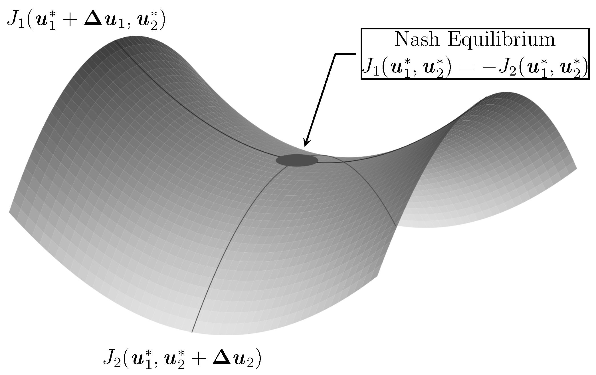
Table 1.
A list of the most important notations used in this survey.
| Item | Definition |
|---|---|
| State | |
| Action | |
| Reward | r |
| Stochastic Transition Matrix | |
| Transition probability | |
| Horizon | T |
| Uncertainty | |
| Objective | |
| Bellman Operator | |
| History | |
| Parameter | |
| Value Function | V |
| Q Function | Q |
| Policy/Strategy | |
| Discount Factor | |
| Expectation | |
| Variance | |
| Identity Matrix | |
| Probability Distribution | |
| Learning Rate | |
| Adversary | A |
| Protagonist | P |
Table 2.
Similarities in the notations of reinforcement learning and optimal control. Here the transfer function of reinforcement learning is formulated in discrete time while the dynamics in optimal control are in continuous time.
Table 2.
Similarities in the notations of reinforcement learning and optimal control. Here the transfer function of reinforcement learning is formulated in discrete time while the dynamics in optimal control are in continuous time.
| Reinforcement Learning | Optimal Control |
|---|---|
| State | State |
| Action | Control |
| Reward r | Cost |
| Observations o | Measurements y |
| Transition | Dynamics |
Publisher’s Note: MDPI stays neutral with regard to jurisdictional claims in published maps and institutional affiliations. |
© 2022 by the authors. Licensee MDPI, Basel, Switzerland. This article is an open access article distributed under the terms and conditions of the Creative Commons Attribution (CC BY) license (https://creativecommons.org/licenses/by/4.0/).
Share and Cite
MDPI and ACS Style
Moos, J.; Hansel, K.; Abdulsamad, H.; Stark, S.; Clever, D.; Peters, J. Robust Reinforcement Learning: A Review of Foundations and Recent Advances. Mach. Learn. Knowl. Extr. 2022, 4, 276-315. https://doi.org/10.3390/make4010013
AMA Style
Moos J, Hansel K, Abdulsamad H, Stark S, Clever D, Peters J. Robust Reinforcement Learning: A Review of Foundations and Recent Advances. Machine Learning and Knowledge Extraction. 2022; 4(1):276-315. https://doi.org/10.3390/make4010013
Chicago/Turabian StyleMoos, Janosch, Kay Hansel, Hany Abdulsamad, Svenja Stark, Debora Clever, and Jan Peters. 2022. "Robust Reinforcement Learning: A Review of Foundations and Recent Advances" Machine Learning and Knowledge Extraction 4, no. 1: 276-315. https://doi.org/10.3390/make4010013