In this section, we change focus from advice production to advice distribution: learning a teaching policy in order to most effectively distribute the advice budget.
5.1. Constrained Exploitation Reinforcement Learning
We attempt a more natural formulation of the AuB learning problem described in
Section 3.2 by identifying it as an instance of a more generic reinforcement learning problem. This RL problem can be simply described as learning control with constraints imposed on the
exploitation ability of the learning agent. These constraints can either be a finite number of times the agent can exploit using its policy, possibly states where it is only allowed to explore, or even perhaps a task where it is costly to have access to an optimal policy and we are allowed to use it only for a limited number of times. How does this RL problem relate to the learning to teach problem? The first insight is that the advise/not advise decision problem has a striking resemblance to the core exploration–exploitation problem of RL agents. Consider the learning to teach problem. We can view the problem as follows: when the teacher agent is advising, it is actually acting on the environment; this is because an obedient student agent will always apply its advice, thus becoming a deterministic actuator for the teacher. In the case of a non-obedient student, the teacher could be said to be using a stochastic actuator.
Consequently, we can view the teacher agent as an acting agent using a student agent as its actuator for the environment. Moreover, the teacher is acting greedily by advising his/her best action; thus, he/she exploits. Under this perspective, with advice seen as action, how could we view the no advice action of a teacher? The no advice action can be seen as “trusting” the student to control the environment autonomously. Thus, choosing not to advise in a specific state can be seen as denoting that state to be non-critical with respect to the remaining advice budget and the student’s learning progress, or denoting a lack of teacher’s knowledge for that state. From the teacher’s point of view, not advising can be seen as an exploration action. Thus, controlling when not to advise can be seen as a directed exploration problem in MDPs. Imposing a budget constraint, which is a constraint on the number of times a teacher agent can advise (i.e., exploit) is a problem of constrained and directed exploitation.
We will consider a simple and motivating example of such a domain. In a grid world , a robot learns an optimal path towards a rewarding goal state while it should keep away from a specific damaging state. The robot is semi-autonomous; it can either control itself using its own policy or it can be teleoperated for a specific limited number of times. For the robot’s operator, what is an optimal use of this finite number of control interventions? What are the states that it would be best to control the robot directly, leaving control of the rest to the robot?
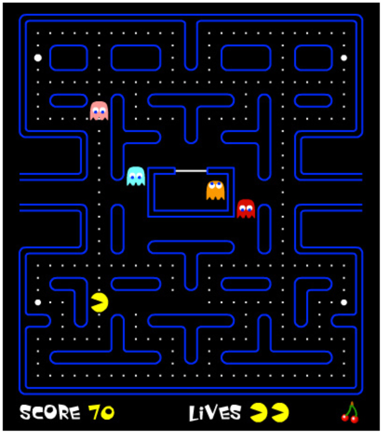
Similarly to the previous example, learning and executing advising policies in a game can be another example of the constrained exploitation problem, which is also the main focus of this article. For example, in a video game like Pac-Man, a game hints system plays the role of the external optimal controller with a limited intervention budget. Such a hint system could suggest actions to human players—when these are most necessary—depending also on the player’s policy.
In the rest of this section, we use the term exploitation where one can think of advising and the term exploration when not-advising, focusing on the broader learning problem.
5.2. Learning Constrained Exploitation Policies
Formulating the constrained exploitation task as a reinforcement learning problem itself first requires defining a horizon for the returns. This horizon should be different from that of the actual underlying task (e.g., Pac-Man) because (a) if the underlying task is episodic, then the scope of an exploration–exploitation policy is naturally greater than that and spans across many episodes of the learning agent; (b) if the underlying task is continuing or requires several training episodes for the student, the exploration–exploitation policy may have to be evaluated in a shorter (finite) horizon (e.g., for the first x training episodes). The importance of exploration is usually limited in the late episode(s) where the student may have already converged to a policy. A teaching policy should be primarily evaluated for a training period where advice still matters.
Concerning the return horizon of a constrained exploitation task (and similarly to [
4] but in a different perspective), we propose algorithmic convergence [
4] as a suitable
stopping criterion when learning an exploration–exploitation policy. This defines a meaningful horizon for exploration–exploitation tasks since their goal is completed exactly then, not in the end of an episode and not in the continuous execution of an RL algorithm—after convergence—where exploration may not affect the underlying policy any more. We proceed by defining the Convergence Horizon Return.
Definition 8 (Convergence Horizon Return). Let G be the return of the rewards received by an exploration–exploitation policy, Q the value function of the underlying MDP and a small constant then:which, for the time step T, applies: Given a small constant and the algorithmic convergence of the RL algorithm learning in the underlying MDP, the quantity . The algorithmic convergence will be realized either if the learning rate is discounted or if some temporal difference of the underlying algorithm tends to .
Using the convergence horizon for the return of a teaching task too, the next question can be what are the rewards constituting the return of a teaching task.
One possible goal for any teacher advising with a finite amount of advice would be to help minimize
student’s regret with respect to the reward obtained by an optimal policy. However, since we do not assume such knowledge, and because there is a finite amount of advice, a better goal could be to advise based on the state-action
value of the advised action and not its immediate
reward. If the student was able to follow the rest of the teacher’s policy after receiving advice, then the action
for the current state
s would be the best possible. Consequently, we define the notion of
value regret.
Definition 9 (Value Regret). In a convergence horizon T, the value regret, of an exploration–exploitation policy (i.e., teaching policy) with respect to both an acting policy obtained after the T period and an acting policy (i.e., student’s policy), , in time step t is:
where
denotes the corresponding value function of
.
The intuition behind this definition of regret in our context (where the acting agent is the student) is that the best teacher for any specific student would ideally be the student himself, when it would have reached convergence or its near-optimal policy.
The important thing to note here is that because a student agent receives a finite amount of advice, he/she cannot improve their asymptotic performance [
4]; consequently, the evaluation of a teaching policy should ideally be based on the student’s optimal policy and not to that of some probably very different teacher because that is its
sustainable optimality.
For example, consider two states in a teacher’s acting MDP, A and B. A student agent learning with a very simplistic state representation may observe these states as just one, C, and not differentiate between them. Then, the student’s optimal action in state C will have a different expected return than that obtained by the teacher from either A or B. Its sustainable optimality is defined as to what is optimal given its simplistic internal representation. Any advice based on a finer representation may not be supported with consistency by the student in the long run. A teaching policy should be ideally evaluated on how much it speeds up the student converging to its own optimal policy.
In the next section, we propose a reward signal for teachers based on Value Regret.
5.3. The Q-Teaching Algorithm
The Q-Teaching algorithm described and proposed in this section is an RL advising (teaching) algorithm learning a teaching policy. For this, we propose a novel reward scheme for the teacher based on the value regret (see Definition 9).
The key insight of the method is that of rewarding a teaching policy with quantities of the form where is an estimation of the student’s action in and is the teacher’s greedy action in (i.e., the action used for advice). This reward has a high value when the value of the greedy action is significantly higher than the value of the action that the student would take. This means that the teacher is encouraged to advise when the advised action is significantly better than the action the student would take.
For terms of efficiency and to emphasize the value impact of the advising action, Q-Teaching rewards all no-advice actions with zero. The advantages of such a scheme is that the teacher’s cumulative reward is based only on the value gain produced when advising and a teaching episode can finish when the budget finishes, not having to observe all the student’s episodes after its budget finishes. From preliminary experiments, rewarding no advice actions too (which occur significantly more than the maximum B advice actions) was overpowering the advice actions, resulting in an imbalanced expression of the two actions in the teaching value function.
Still, when advising, the teacher should estimate
in order to compute its reward. The simplest solution is that, since we do not have access to the value function of the student or its internals, we use the acting value function
of the teacher as an approximation for the optimal value function of the student,
. To estimate
the teacher has several options. If the teacher is notified of the intended action of the student beforehand, it can use that to compute the reward. If we assume no knowledge of the student’s intended action, then some other estimation method for the student’s intended action should be used. An example of such an estimation method is used in the Predictive Advice method [
6].
While predicting the actual student’s action (
) is possible, there are other—simpler—choices for this estimation too. For example, the Importance Advising (see
Section 2.2) uses a very similar quantity for the advising threshold, of the form
. For Importance Advising, we can say that
—it pessimistically assumes the student will take the worst action, representing the risk of the state. The advantage of such an assignment is that it is based on a well-tested criterion [
6] and that it does not need knowledge of the student’s intended action (desirable for most realistic settings). The disadvantage is that we have a less detailed reward, which is also not adapting to the student’s specific necessities but mostly to the domain’s characteristics.
Based on this dichotomy, we propose two versions of Q-Teaching (see Algorithm 1), the off-student’s policy Q-Teaching and the on-student’s policy Q-Teaching. The on-student’s policy Q-Teaching uses the value of the actual student’s action to compute the reward (thus, it is directly influenced by its policy). We can intuitively say that on-student’s policy Q-Teaching will advise when the student is mostly expected to act sub-optimally with respect to the acting value function of the teacher, . On the other hand, the off-student’s policy Q-Teaching uses the criterion discussed above and the teaching policy is not directly influenced by the policy of the student. Specifically, it is rewarding its teaching policy, , at time-step with the Q-value difference of the best action to the worst action, as these were found at time t.
The Q-Teaching algorithm proceeds as follows (see Algorithm 1). A teacher agent enters an RL acting task to learn an acting policy. It initializes two action-value functions, and , the acting value function and the teaching value function, respectively (lines 1–2). Of course, it can also use an existing acting value function.
Being in time step t and state s, the teacher queries its acting value function for the greedy action in that state (line 6). Depending on whether we use the off-student’s policy or the on-student’s policy Q-Teaching, the teacher sets a baseline action, , to either the worst possible action for that state or to the action just announced by the student (lines 7–11).
Then, the teacher chooses an action from
based on
and its exploration strategy. If the teacher chooses to advise (line 13), it gives the action
as an advice to the student agent. If the teacher chooses not to advise, the student will proceed with its own policy.
| Algorithm 1 Q-Teaching |
- 1:
Initialize arbitrarily ▷ teaching value function - 2:
Use existing or initialize it ▷ acting value function - 3:
repeat (for each teaching episode) ▷ teacher–student session - 4:
Initialize s - 5:
repeat (for each step) - 6:
- 7:
if (Off-Student’s policy Q-Teaching) then - 8:
- 9:
else - 10:
▷ where a is the action announced by the student - 11:
end if - 12:
Choose from using policy derived from (e.g. -greedy) - 13:
if = {advice} then - 14:
Advice the student with the action - 15:
▷ update remaining budget - 16:
else if = {no_advice} then - 17:
Send a ⊥ (no advice message) to the student - 18:
end if - 19:
Observe student’s actual action a and its new state and reward, - 20:
▷ possibly continue learning an acting policy - 21:
if = {advice} then - 22:
- 23:
else if = {no_advice} then - 24:
- 25:
end if - 26:
- 27:
- 28:
until OR teacher reached the estimated convergence horizon episode of the student - 29:
until end of teaching episodes
|
On line 19, the teacher observes the student’s actual action a and its new state and reward, . Once again, the student may be the teacher himself; in this case, it observes its own action that was taken based on and its exploration strategy.
On line 20, the first Q-Learning update takes place for the acting value function based on the environment’s reward. For the teaching value function update, the teacher’s reward, is calculated first, based on the freshly updated values of the best and baseline actions, and respectively (lines 21–25).
Finally, a Q-Learning update for the teaching value function takes place based on the reward (line 26) and the algorithm continues in the same way until whatever of the following two events comes first: either the advice budget finishes or the student reaches a learning episode that we have predetermined as its convergence horizon. These complete one learning episode or session for the teacher.
In this version, the Q-Teaching algorithm is based on the Q-Learning algorithm, although, in principle, any RL algorithm could be used for the underlying learning updates of Q-Teaching. However, if an off-policy RL algorithm such as Q-Learning is chosen for the updates of both the acting and the teaching value function, then the point of transition from acting to teaching is irrelevant to the learning progress of the two policies. Reducing the impact of the exploration policy to the learning updates allows for smoother interaction between the two policies and ensures us that we continue to learn the same policies. In principle, a Q-Teaching agent is able to update both its acting and teaching value functions continually and refine not only when it should advise but also what it should advise.
Since our goal is to introduce Q-Teaching as a flexible and generic enough method to be applied to multiple domains, we propose a series of state features for the teaching task state space that we think are necessary. From our experiments, Q-Teaching works best with an augmented version of the acting task state space (see
Table 3) similar to that of [
5] (Zimmer’s method). Also in
Table 3, note the role of the student’s progress feature (
): it homogenises the student’s Markov chain by inducing a state feature for time (see
Section 3.2).
5.4. Experiments and Results
In this section, we present results from using Q-Teaching in the Pac-Man Domain. We evaluate both on-student’s policy Q-Teaching and off-student’s policy Q-Teaching, in two variations each: known or unknown student’s intended action. Note that methods like Zimmer’s and Mistake Correcting require knowledge of the student’s intended action.
We use two versions of students for the experiments. A low-asymptote and a high-asymptote Sarsa students. Referring to [
6] and
Section 2.3, the low asymptote students receive a state vector of 16 primitive features related to the current game state while the high asymptote students receive a state vector of seven highly engineered features providing more information [
6]. The low-asymptote students have significantly worse performance than the high-asymptote ones.
Additionally, we choose to bootstrap all compared teaching methods with the same acting policy in order to equally compare their advice distribution performance and not their quality of the advice. The acting policy used for producing advice comes from a high-asymptote Q-Teaching agent after 1000 episodes of learning. Moreover, we use Sarsa students in order to emphasize the ability to advise students that are different to the teacher. All learning methods (Zimmer’s and Q-Teaching) were trained for 500 teaching episodes (sessions) to be equally compared for their learning efficiency too.
The Q-Teaching learning parameters for the teaching policy were
, decaying
and
whereas all Sarsa students had
,
and
. The evaluation was based on the student performance (game score) and using the
Total Reward TL metric [
2] divided by the fixed number of training episodes. The student performance is evaluated every 10 advising episodes (while learning) for 30 episodes of acting alone (and not learning). For the comparisons between average score performances, we used pairwise
t-tests with Bonferroni correction [
18]. Statistically significant results are denoted with their significance level and they always refer to paired comparisons.
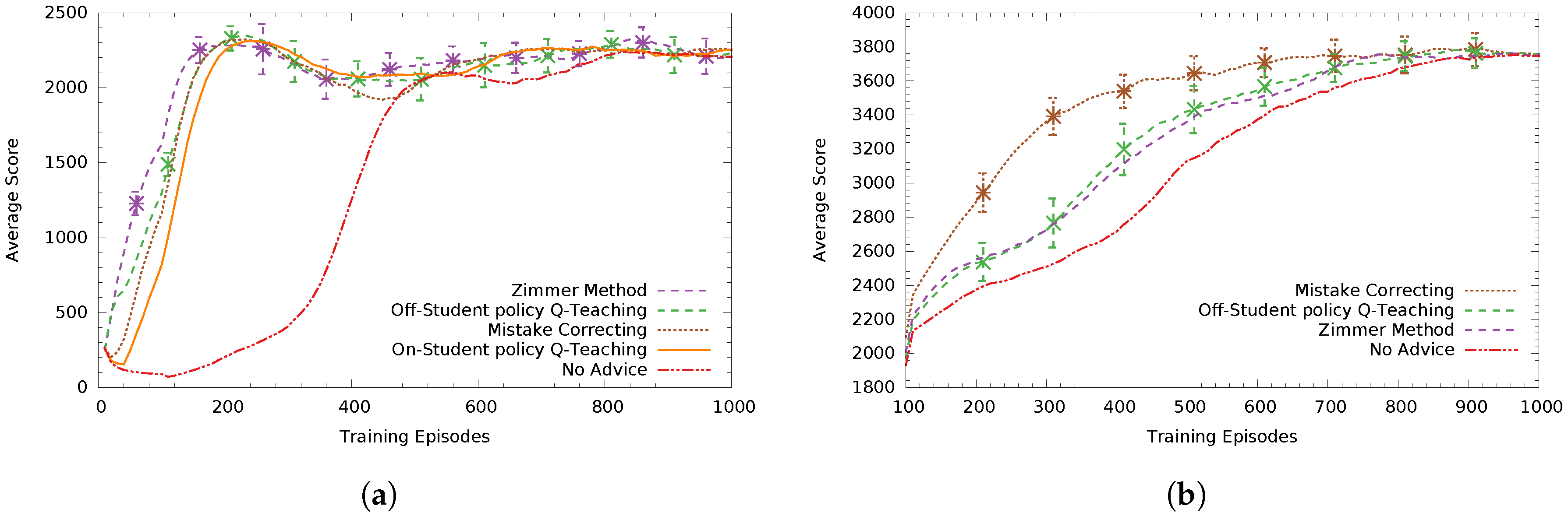
In
Figure 4a, teacher agents advise a low-asymptote Sarsa student who always announces its intended action. We can see Zimmer’s method performs best and off-student’s policy Q-Teaching comes second with a statistically significant difference (
). The heuristic based-method Mistake Correcting with a tuned threshold value of
comes third. On-student’s policy Q-Teaching performed worse than the previous three methods by a small margin, having not found an as good advice distribution policy (non-significant difference to Mistake Correcting). Finally, all methods performed statistically significantly better (
) than not advising, effectively speeding up the learning progress of the student.
In
Figure 4b, the teachers advise a high-asymptote Sarsa student. Here, the tuned version of Mistake Correcting (
) performed statistically significantly better (
) than all methods, with Q-Teaching methods coming second and third (respectively) and Zimmer’s method coming next (having non-significant differences between them).
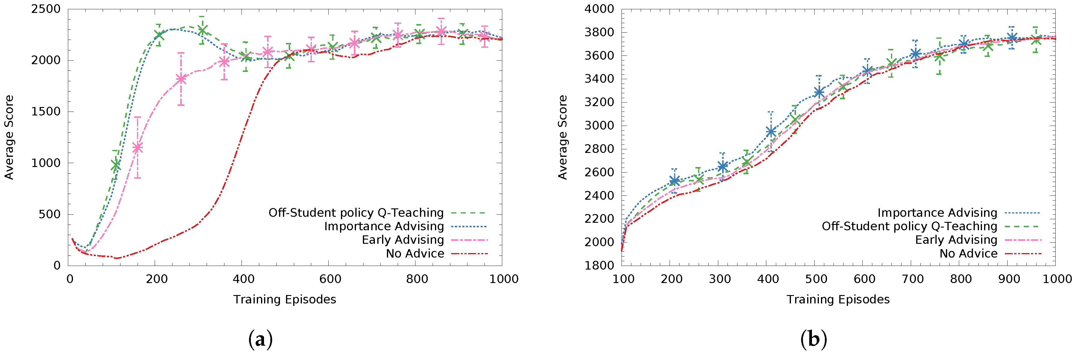
For the case when the teacher agent is not aware of the student’s intended action (see
Figure 5), in
Figure 5a the off-student-policy Q-Teaching performs best while Importance Advising (
) follows with a small performance difference (non significant). Early Advising (giving all
B advice in the first
B steps) performs statistically significantly worse (at
) than both Q-Teaching and Importance Advising. In these experiments, we did not use on-student’s policy Q-Teaching since that requires knowing the student’s intended action to compute the reward.
In
Figure 5b, advising a high asymptote Sarsa student, Q-Teaching had the second best performance with the heuristic-based method importance advising (
) performing better (non significant). For high performing students, a poorly distributed advice budget can be much less effective. For example, if the teacher knows the student’s intended action, it does not spend advice in states where the student would anyway choose the correct action. This fact is emphasized in this specific case, since no advising did not perform significantly worse compared to the rest of the methods.
Finally, in
Table 4 and
Table 5, we can see the average total reward in 1000 training episodes for all of the teaching methods. All methods knowing the student’s intention performed better than those that did not, taking advantage of that knowledge.
Q-Teaching, the only learning AuB method allowing students to not announce their intended action, performed relatively well compared to methods that know the student’s intended action, which is an advantage of the proposed method.
Most importantly, while Zimmer and Q-Teaching methods were both trained for 500 episodes (sessions), Q-Teaching training was completed significantly faster since the Zimmer method has to observe all 1000 episodes of each student session to complete just one of its own, whereas Q-Teaching has an upper bound for its episode completion. This upper bound is the algorithmic convergence of the student (e.g, the low-asymptote student requires only 500 episodes to converge) and, in most cases, it will be completed much faster, when the budget finishes (around the 30th episode for the low-asymptote student). More specifically, in
Table 4 and
Table 5, we can see the average training time needed for each teacher (in terms of the average observed
student episodes) in each of the 500 teacher episodes. In general, our proposed methods need at least
less training time than the Zimmer’s method. We should also note here that, although non-learning methods do not need training time, they require a significant and variable amount of manual parameter tuning to achieve the reported performance.
Another advantage of off-student’s policy Q-Teaching is that it can use the same teaching policy for very different students since it is not directly influenced from the student’s policy and the rewards received by the student when not advising (such as in the Zimmer method). This is a significant advantage in terms of learning speed and versatility since heuristic methods have to be manually tuned for each student separately to find the optimum threshold, t.
On-student policy Q-Teaching did not perform as well as expected, the main problem being the non-stationary reward depending on the student’s changing policy. We believe that this method needs significantly more training time than the off-student’s policy Q-Teaching because of its non-stationary reward and it probably needs more informative features for the student’s current status. In our case, this was only its training episode, which is the most basic information available for the student. Moreover, the training episode feature is student-dependent since its meaning varies among students—some students learn faster than others.


