An Algorithm for Generating Invisible Data Poisoning Using Adversarial Noise That Breaks Image Classification Deep Learning

Abstract

Today, the main two security issues for deep learning are data poisoning and adversarial examples. Data poisoning consists of perverting a learning system by manipulating a small subset of the training data, while adversarial examples entail bypassing the system at testing time with low-amplitude manipulation of the testing sample. Unfortunately, data poisoning that is invisible to human eyes can be generated by adding adversarial noise to the training data. The main contribution of this paper includes a successful implementation of such invisible data poisoning using image classification datasets for a deep learning pipeline. This implementation leads to significant classification accuracy gaps.

1. Introduction

Today, it seems that deep learning (which appears for computer vision in [1], see [2] for a review) may lead to a major industrial revolution. Applications already go much further than social networking [3] and include autonomous driving [4], healthcare [5], plagiarism detection [6], and security (e.g., [7]).

However, classical deep networks lack robustness. Indeed, classical networks admit adversarial examples [8,9,10,11]. At test time, it is possible to design a specific invisible perturbation, such as the network predicting different outputs between the original and disturbed input. For instance, [12] highlights this issue in the cybersecurity context. A deep learning system is designed to detect malwares from large app repository (like an Android app). This network reaches a state-of-the-art detection performance of 87%, but detection performances drop to only 66% for adversarial malwares (let us stress that the production of adversarial examples does not require access to the internal structure of the network [13,14]).

On a static problem, adversarial examples are not an issue because the goal is more to generalize (understanding the underlying semantic) than to be robust (still recognizing under unusual noise). Of course, both properties are correlated, but generalization is more a matter of affinity between the algorithm and the targeted data distribution than a property of the algorithm itself (see [15] for illustration). So, as the adversarial examples do not belong to this targeted distribution, it is not so surprising that the network may badly handle such outliers. Now, adversarial examples are a critical issue for real-life applications of deep learning: indeed, if a deep network is deployed in the real world, people will interact with it. So, the network may have to face hacking attacks which can take the form of adversarial examples (which can be produced in the physical world [16]).

Another critical issue with deep learning is data poisoning [17]. Data poisoning is a field of cybersecurity. The goal of such attacks is to pervert a learning system by manipulating a small subset of the training data. Data poisoning could be a serious threat to deep learning-based malware detection. Indeed, the system will be trained on a large and uncontrolled set of software produced by other people (some of who may be hackers). Thus, it will be important not to forget that one could have introduced a few data-poisoned samples to the training data. In particular, training processes for deep learning do not form hypotheses about the integrity of the training data. In addition, [18] shows that deep learning is sensitive to such attacks: on MNIST, [18] reports the ability to make the error jump from 1.3% to 2% and 4% just by manipulating 3% and 6% of the training dataset.

So, deep networks are sensitive both to adversarial examples and data poisoning. Furthermore, in this paper, I show that the two issues can be combined to create a third one: data poisoning that is invisible to human eyes can be generated by adding adversarial noise to the training data. The main contribution of this paper is the efficient implementation of invisible data poisoning based on adversarial example algorithms, and thus, the demonstration that such a phenomenon could be critical.

As a prelude, the proposed invisible data poisoning allows for the capability of changing the accuracy of classical deep networks by more than 30% using the well-known dataset CIFAR100 [19] with a 1% modification at the pixel level.

In the next section, I present a quick overview of adversarial examples and data poisoning. Then, I present the proposed algorithm to produce invisible data poisoning. Then, in Section 4, I present empirical experiments evaluating the potential impact of this adversarial-based data poisoning, before a conclusion and perspectives in Section 5.

2. Related Work

2.1. Why Such Robustness Faults?

A classical deep network is a sequence of simple tensor operations done from an input. So, as stressed by [11], classical deep networks are a Lipschitz function expected to be smooth. Now, the problem is that the Lipschitz coefficient is large. For instance, the Frobenius norm of the first deep network Alexnet [1] is 5,908,006,809. So, if a deep network is just a sequence of simple operations, the number of parameters (and the amplitude of these parameters) coupled with the large number of layers leads to a potentially very unsAlgorithm output compared to other machine learning algorithms e.g., support vector machine (SVM) [20].

However, worse, deep learning is more derivable, allowing hackers to take advantage of this fault. Indeed, this fault is deep-rooted in the back-propagation of the gradient [21], i.e., the core of the training process. Back-propagation allows for computing the derivative according to each weight given a loss from the last layer. However, this relies on the computation of the derivative according to each neuron. Thus, by design, back-propagation allows for computing the derivative according to the input data itself (this can be done easily with PYTORCH pytorch.org/ by just asking the internal variable corresponding to the input to store the gradient). So, the same process which allows the update of the weights according to an input can be used to update the input itself. Thus, one can use gradient descent from a specific input to minimize the probability of the truth class, eventually producing an adversarial example.

This is why adversarial examples are mainly a deep learning issue, even if, technically, adversarial examples may exist for all machine learning algorithms.

In addition, as training is usually done by stochastic gradient descent on a loss which just compares provided and predicted labels, deep learning training does not raise concerns about the provided labels and/or samples at the training stage. Indeed, due to the time needed to train such networks, using an algorithm like RANSAC [22] to detect outliers in the training set is unrealistic. Thus, deep learning algorithms like SVM are structurally sensitive to data poisoning [23].

Again, this problem is strengthened for deep learning, because, as deep learning is derivable, producing data poisoning can be done easily by gradient descent methods [18].

2.2. Formal Presentation

2.2.1. Data Poisoning

The most classical data poisoning task consists of manipulating freely a small subset of the training data; as such, when trained on these data, the targeted system will have a low testing accuracy.

Let F be the learning system to be poisoned: given a set of weights $\theta$ and an input $\mathsf{\Lambda }$, the system returns a predicted classification $F(\mathsf{\Lambda },\theta )$. Then, let ${\mathsf{\Lambda }}_1,\dots ,{\mathsf{\Lambda }}_N$ be the training data associated to the label $y_1,\dots ,y_N$. Let $\mathcal{A}$ be the learning process (which is technically not a function but is written as one for simplification). So, $\mathcal{A}({\mathsf{\Lambda }}_1,\dots ,{\mathsf{\Lambda }}_N,y_1,\dots ,y_N)$ produces weights (i.e., $\theta$ in previous equations). Let $accuracy(\theta )$ be the accuracy on the test set of the system when parameterized with the weights $\theta$. In the most classical task of data poisoning, hackers want to minimize the testing accuracy by freely modifying k training samples over a training set of size $N\gg k$. This corresponds to solving: ${\displaystyle \underset{{\mathsf{\Lambda }}_1^{\prime },\dots ,{\mathsf{\Lambda }}_k^{\prime },y_1^{\prime },\dots ,y_k^{\prime }}{min}}accuracy(\mathcal{A}({\mathsf{\Lambda }}_1^{\prime },\dots ,{\mathsf{\Lambda }}_k^{\prime },{\mathsf{\Lambda }}_{k+1},\dots ,{\mathsf{\Lambda }}_N,y_1^{\prime },\dots ,y_k^{\prime },y_{k+1},\dots ,y_N))$.

Classically, hackers can use any available information, including all knowledge from training and testing datasets, but have only a small subset ($k\ll N$) of the training data under their control.

Alternative tasks (outside the scope of this paper) exist, like reducing the accuracy of specific classes and/or minimizing the number of samples to achieve a target accuracy and/or adding constraints to the poisoned samples and/or having to compute the poisoning without knowledge from the test set, and so on.

2.2.2. Adversarial Examples

A deep learning system is a sequence of simple tensor operations. For example, one can consider the typical case of a multilayer perceptron (MLP). Let h be a simple nonlinear function. The most classical is now the ReLU function, i.e., $h\left(u\right)=max(0,u)$. To simplify, $\widehat{h}$ will be the operator applying h to each cell of any input tensor (i.e., $\forall Q$, ${(\widehat{h}\left(Q\right))}_u=h\left(Q_u\right)$, with u as a set of indexes). The weights of an MLP are a set of matrices $\theta =\left(M_1,M_2,\dots ,M_R\right)\in M_{n_1,m_1}\times \dots \times M_{n_R,m_R}$, with $m_1=D$, $n_r=m_{r+1}$, and $n_R$ being the desired output size of the network. Finally, for an input $\mathsf{\Lambda }\in {\mathbb{R}}^D$, the MLP output is just $F(\mathsf{\Lambda },\theta )=M_R\widehat{h}\left(M_{R-1}\widehat{h}\left(\dots M_2\widehat{h}\left(M_1\mathsf{\Lambda }\right)\right)\right)$.

Such an MLP is a Lipschitz function: there exists a constant $\Omega$, such that $\forall \mathsf{\Lambda },\delta \in {\mathbb{R}}^D$, $\left|\right|F(\mathsf{\Lambda },\theta )-F(\mathsf{\Lambda }+\delta ,\theta )\left|\right|\le \Omega \left|\right|\delta \left|\right|$. Yet, $\Omega \le \rho (M_R)\times \dots \times \rho (M_1)$, where $\rho$ is the operator norm (here, the largest eigenvalue), and so it could be very large, leading to an unsAlgorithm output.

Let $B_{ϵ}=\{u,|\left|u\right||\le ϵ\}$ (typically, $ϵ$ is an input ensuring that an $ϵ$ perturbation is invisible). The unsAlgorithm behavior of deep learning means than for (almost) all input $\mathsf{\Lambda }$, one may find invisible noise ${\delta }_{\mathsf{\Lambda }}^{adverse}\in B_{ϵ}$ such that $\left|\right|F(\mathsf{\Lambda },\theta )-F(\mathsf{\Lambda }+{\delta }_{\mathsf{\Lambda }}^{adverse},\theta ){\left|\right|}_2$ is very large. In the classification context, one may find ${\delta }_{\mathsf{\Lambda }}^{adverse}$, such as $\mathsf{\Lambda }+{\delta }_{\mathsf{\Lambda }}^{adverse}$, is badly classified.

If the network is a white box, a very simple Algorithm 1 to generate such an adversarial example is just:

Algorithm 1: A simple baseline to generate adversarial examples

adversarialGeneratorBaseline:   let $loss$ be the loss function   while not meeting a stopping criterion    compute $loss(F(\mathsf{\Lambda },\theta ))$    compute derivatives on $\mathsf{\Lambda }$    update $\mathsf{\Lambda }$ to increase the loss

Adversarial attacks are very impressive, especially in computer vision where small perturbations of images are usually undetecAlgorithm to human eyes. Examples of modified images are given in Section 4.

Yet, to highlight the classical statement that a small perturbation of an image is not detected by the human eye, I propose to consider Figure 1: it should be hard for a human to discern between the first four images of this figure. Yet, between these images, a modification of amplitude 20 over 255 is allowed, while classical adversarial attacks may have a very low amplitude (e.g., between 0 and the $\pm 5$ images in the Figure 1). This is also the case in the proposed experiments in Section 4.

3. Adversarial-Based Invisible Data Poisoning

In the previous section, data poisoning and adversarial examples are presented. Here, I introduce invisible data poisoning, and then, I present how algorithms initially designed to produce adversarial examples can be modified to produce such invisible data poisoning.

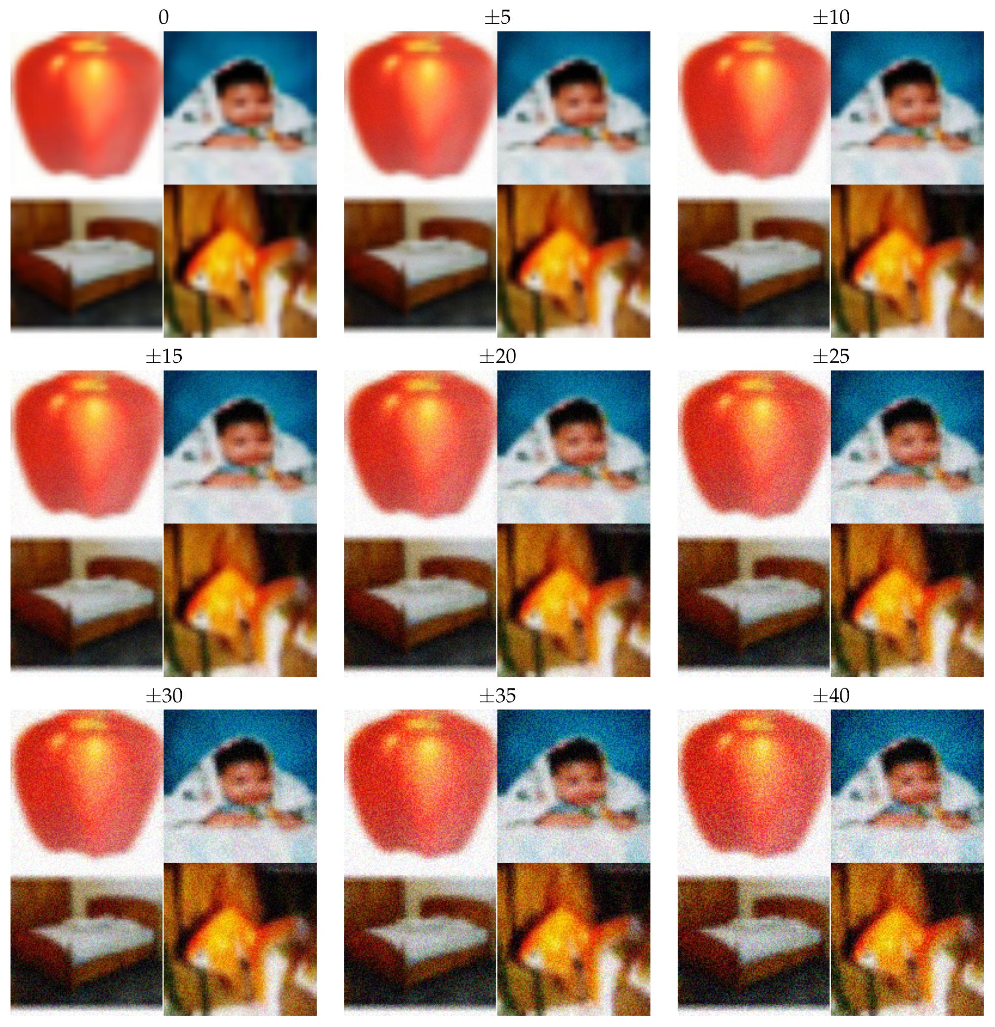
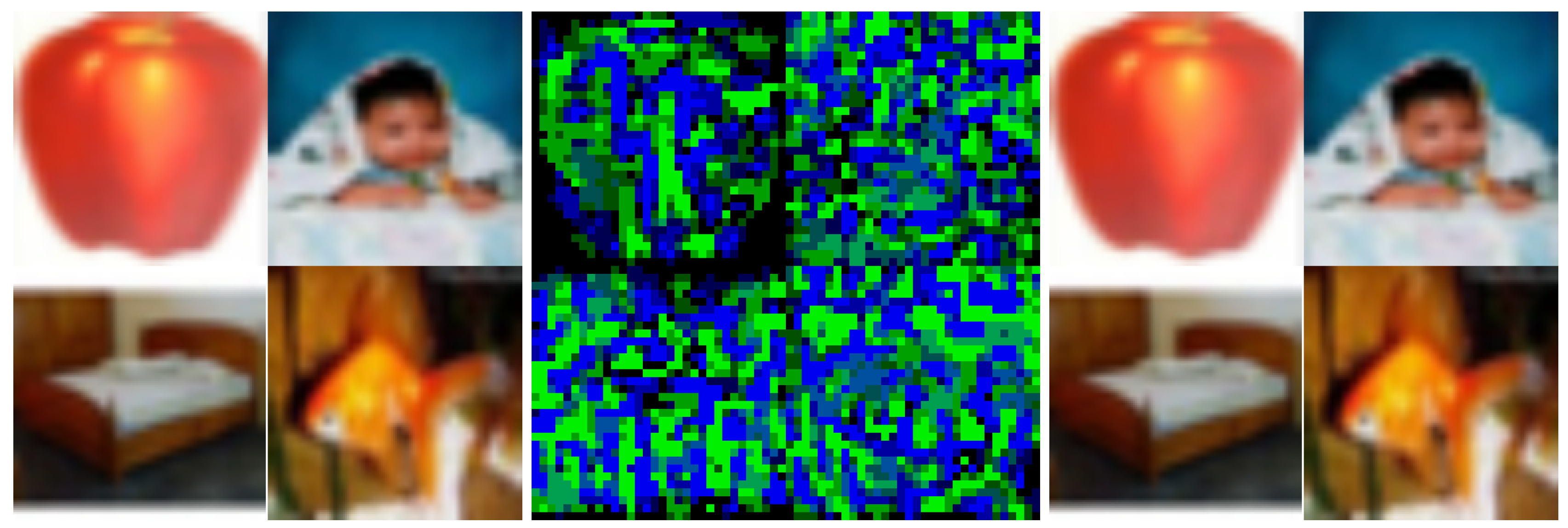
3.1. Invisible Data Poisoning

Invisible data poisoning is a derived task of designing data poisoning, with the constraint that the perturbation of the samples should be small (in image context, invisible to human eyes).

So, to recall, classical data poisoning consists of solving ${\displaystyle \underset{{\mathsf{\Lambda }}_1^{\prime },\dots ,{\mathsf{\Lambda }}_k^{\prime },y_1^{\prime },\dots ,y_k^{\prime }}{min}}accuracy(\mathcal{A}({\mathsf{\Lambda }}_1^{\prime },\dots ,{\mathsf{\Lambda }}_k^{\prime },{\mathsf{\Lambda }}_{k+1},\dots ,{\mathsf{\Lambda }}_N,y_1^{\prime },\dots ,y_k^{\prime },y_{k+1},\dots ,y_N))$.

However, I introduce in this paper invisible data poisoning, which instead consists of solving: ${\displaystyle \underset{{\delta }_1,\dots ,{\delta }_k\in B_{ϵ}}{min}}accuracy(\mathcal{A}({\mathsf{\Lambda }}_1+{\delta }_1,\dots ,{\mathsf{\Lambda }}_k+{\delta }_k,{\mathsf{\Lambda }}_{k+1},\dots ,{\mathsf{\Lambda }}_N,y_1,\dots ,y_N))$.

In other words, invisible data poisoning is a special case of data poisoning where the training labels cannot be changed and where poisoned samples are constrained to be very close to the corresponding original samples (alternative data poisoning tasks, like minimizing the accuracy of a given class, may be translated into an alternative invisible data poisoning task).

Of course, invisible data poisoning is less efficient than classical data poisoning. Yet, the hacker knows that before running the training, the target dataset will be reviewed by an expert. Then, there is absolutely no chance to poison the dataset by changing a label (the expert will see the wrong labeling) or by adding a large deformation (the expert will see the unrealistic nature of the data). This is especially the case if it is an image dataset. So, invisible data poisoning is the only realistic poisoning strategy when data are reviewed by a human.

3.2. Using Adversarial-Like Noise

Now, looking simultaneously at the equation of invisible data poisoning from the previous subsection, as well as at the presentation of adversarial examples (Section 2.2.2), a very natural and straightforward idea underlying a poisoning is to examine the formula $accuracy(\mathcal{A}({\mathsf{\Lambda }}_1+{\delta }_{{\mathsf{\Lambda }}_1}^{adverse},\dots ,{\mathsf{\Lambda }}_k+{\delta }_{{\mathsf{\Lambda }}_k}^{adverse},{\mathsf{\Lambda }}_{k+1},\dots ,{\mathsf{\Lambda }}_N,y_1,\dots ,y_N))$.

Yet, this idea should be improved if it is to become an efficient attack because all noises ${\delta }_{\mathsf{\Lambda }}^{adverse}$ should cooperate, rather than just having a separate influence on each poisoned sample. So, the idea is to try to compute ${\delta }_1,\dots ,{\delta }_k$ so that the noises are computed with algorithms derived from adversarial examples but also collectively designed to minimize the testing accuracy. Let us add an exponent $adversepoisoning$ to stress that the noise is obtained thanks to adversarial example algorithms. So, combining invisible data poisoning and adversarial examples consists of instead considering the problem: ${\displaystyle \underset{{\delta }_1,\dots ,{\delta }_k\in B_{ϵ}}{min}}accuracy(\mathcal{A}({\mathsf{\Lambda }}_1+{\delta }_1^{adversepoisoning},\dots ,{\mathsf{\Lambda }}_k+{\delta }_k^{adversepoisoning},{\mathsf{\Lambda }}_{k+1},\dots ,{\mathsf{\Lambda }}_N,y_1,\dots ,y_N))$.

3.3. The Return Favor Algorithm

The major contribution of this paper is to propose an efficient algorithm to produce such noise as described above (The proposed algorithm is empirically efficient, but it does not come with theoretic justification. In Appendix A, I give an algorithm for a very restricted case, but it comes with interesting theoretic properties.). This algorithm is called the return favor algorithm in this paper.

3.3.1. Requirements

The proposed algorithm:

• works in binary or multi-class contexts
• works on both integer and real data
• is not restricted to a specific data poisoning context: no constraint on k, no constraint on the loss (i.e., generic accuracy minimization or specific class accuracy minimization), etc.
• needs some desired weights ${\theta }^{poison}$ as input
• works with a deep network plus SVM pipeline [24]

The desired weights ${\theta }^{poison}$ required as input allow moving from the problem ${\displaystyle \underset{{\delta }_1,\dots ,{\delta }_k\in B_{ϵ}}{min}}accuracy(\mathcal{A}({\mathsf{\Lambda }}_1+{\delta }_1^{adversepoisoning},\dots ,{\mathsf{\Lambda }}_k+{\delta }_k^{adversepoisoning},{\mathsf{\Lambda }}_{k+1},\dots ,{\mathsf{\Lambda }}_N,y_1,\dots ,y_N))$ to a simpler problem where accuracy has been removed (this is interesting, as accuracy is not smooth): ${\displaystyle \underset{{\delta }_1,\dots ,{\delta }_k\in B_{ϵ}}{min}}\left|\right|{\theta }^{poison}-\mathcal{A}({\mathsf{\Lambda }}_1+{\delta }_1^{adversepoisoning},\dots ,{\mathsf{\Lambda }}_k+{\delta }_k^{adversepoisoning},{\mathsf{\Lambda }}_{k+1},\dots ,{\mathsf{\Lambda }}_N,y_1,\dots ,y_N))||$. Here, minimizing the difference can be replaced by maximizing the cross-product in this context, as weights produced by $\mathcal{A}$ are more or less normalized.

The weights ${\theta }^{poison}$ can be obtained by the hacker by any means, e.g., from knowledge on the testing data. Of course, ${\theta }^{poison}$ should verify $accuracy({\theta }^{poison})\ll 1$ (hence, being increasingly closer to ${\theta }^{poison}$ should lead to a decreasingly lower accuracy). These desired weights are a bottleneck in the proposed pipeline. Yet, the classical scenario of data poisoning is when training data are owned and testing data are known but not owned. In this case, ${\theta }^{poison}$ can be obtained easily.

The pipeline deep network plus SVM is introduced in [24]. It is common when reusing a deep network trained on a large dataset to train a specific SVM for a new task on a smaller dataset from an intermediary output of the network. This corresponds to training only the last layer for a new task while keeping all the other layers unchanged. This pipeline deep network plus SVM is restricted (training the last layer instead of all). Yet, one advantage is the possibility of allowing reproducible experiments (as the training of the last layer only is a convex problem, two instances of training should lead to the same weights). In any case, the deep network plus SVM is common on small real-life problems.

3.3.2. Pseudo-Code

First, Algorithm 2 presents the fair training procedure in the specific case of a deep network plus SVM. In other words, Algorithm 2 corresponds to $\mathcal{A}$ in all the previous equations. Consistent with the data poisoning context, $\mathcal{A}$ is a fair algorithm used by the victim.

Then, Algorithm 3 presents the proposed invisible data poisoning algorithm, i.e., the algorithm that hackers would apply to the subset of the dataset which is under their control after having computed, by any means, some target weights ${\theta }^{poison}$.

The algorithm can be described this way. First, an auxiliary network composed of the network plus the last layer initialized with ${\theta }^{poison}$ is created (notice that the goal of the hacker is that the victim gets exactly these weights after a fair training on the poisoned dataset). Then, for each training data, forward–backward is computed with this auxiliary network to collect the derivative corresponding to the data (not to the weights of the network). Then, each data value is updated either with the sign of the corresponding derivative in the integer case or with the derivative in the floating case. This way, the algorithm creates modified training data with each value having a distance of at most 1 from the original value in the integer case.

The underlying idea is to modify the training samples to increase the score given to them by the desired weights, because, eventually, in return, training on these modified samples leads to the desired weights. This is why this algorithm is called the return favor algorithm. This idea is a way to remove $\mathcal{A}$ from the equation to be solved ($accuracy$ having being removed by the introduction of ${\theta }^{poison}$). This assumption of favor return is far from trivial and is experimentally verified in following experiments.

Algorithm 2: Pseudo-code of a fair training of the last layer of a network.

fairLastLayerTraining(CNN,X,Y)   theta = randomVect()   pipeline = CNN::theta   for epoch in nbEpoch:    shuffle(X,Y)    for x,y in X,Y:     gradient = forwardBackward(pipeline,x,y,crossentropy)     theta -= lr*gradient[w]   return theta

Algorithm 3: Pseudo-code of the return favor algorithm.

//Here, X corresponds to the subset of the dataset  //which is over the control of the hacker.  //Output is X’ a modified dataset.  //Applying a fair training process on the dataset X’,Y  //leads to a model biased toward thetaPoison.  returnFavorAlgorithm(CNN,thetaPoison,X,Y)   auxiliaryCNN = CNN::thetaPoison   X’ = []   for x,y in X,Y:    gradient = forwardBackward(auxiliaryCNN,x,y,crossentropy)    if data type is integer     x’ = x + sign(gradient[x])    else     x’ = x + gradient[x]/norm(gradient[x])    X’.append(x’)   return X’

3.3.3. Key Points of the Algorithm

Loosely speaking, a difficulty in adversarial-based data poisoning is that one aims to modify training samples (individually) in order to decrease testing accuracy. Yet, the link between one training sample modification and the testing accuracy is too weak. So, there is a need for a proxy to go from global (testing accuracy) to local (each training sample modification).

The return favor algorithm uses two ideas to implement such a proxy:

• desired weights allow for capturing of testing accuracy behavior (approximating $accuracy$ in the general equation in Section 3.2)
• scoring the training samples with the auxiliary network allows for capturing the training behavior (approximating $\mathcal{A}$ in the general equation in Section 3.2)

To give a very brief summary:

The goal of invisible data poisoning is to solve:

${\displaystyle \underset{{\delta }_1,\dots ,{\delta }_k\in B_{ϵ}}{min}}accuracy(\mathcal{A}({\mathsf{\Lambda }}_1+{\delta }_1,\dots ,{\mathsf{\Lambda }}_k+{\delta }_k,{\mathsf{\Lambda }}_{k+1},\dots ,{\mathsf{\Lambda }}_N,y_1,\dots ,y_N))$.

Desired weights allow a first approximation:

${\displaystyle \underset{{\delta }_1,\dots ,{\delta }_k\in B_{ϵ}}{max}}\left|\right|{\theta }^{poison}-\mathcal{A}({\mathsf{\Lambda }}_1+{\delta }_1^{adversepoisoning},\dots ,{\mathsf{\Lambda }}_k+{\delta }_k^{adversepoisoning},{\mathsf{\Lambda }}_{k+1},\dots ,{\mathsf{\Lambda }}_N,y_1,\dots ,y_N))||$ which is then approximated by the return favor algorithm (Algorithm 3).

4. Experiments

In this section, the efficiency of the proposed algorithm is shown empirically (see Appendix A for another algorithm which comes with theoretic properties).

4.1. Datasets

I employed computer vision experiments in order to have classical material, and thus, reproducible experiments. However, the proposed algorithm is not restricted to this use case. So, the data $\mathsf{\Lambda }$ are now images, and the data values are now a set of pixel values. Also, in this case, each pixel should have an integer value.

For these experiments, I applied the CIFAR10 and CIFAR100 datasets, two very classical image datasets [19] (first introduced in 2009 in a technical report learning-features-2009-TR.pdf, available from www.cs.toronto.edu/~kriz/). Both datasets can be downloaded (see the page cifar.html from the same website).

4.2. Experimental Setting

The pipeline inspired by [24] is composed of a classical convolutional neural network (CNN) trained on IMAGENET [25], which is used for feature extraction, plus an SVM. The CNN used is some of the first layers of VGG. The weights are IMAGENET ones and are never updated throughout all experiments (even if the gradient is eventually computed to get derivatives relative to the input). IMAGENET weights of the network are available (for example, from here: github.com/jcjohnson/pytorch-vgg). The SVM implemented is LIBLINEAR [26] with bias and default parameters.

Precisely, $\mathcal{A}$ was computed as follow. Features were extracted from images by the network, producing one vector per image. This feature extraction has no parameters, and thus, is completely reproducible (the only possible changes should be due to hardware settings, PYTORCH version, and/or NVIDIA driver). Then, the SVM was optimized on training vectors and used on testing vectors. As SVM learning is a convex problem, multiple runs should converge to the same solution. There are also zero parameters, as only default parameters are used. Typically, $C=1$ as the default parameter of LIBLINEAR. Fair performances before poisoning were 75% of the testing accuracy on CIFAR10 and 53% of the accuracy on CIFAR100 (these performances are quite normal for a pipeline mainly trained on IMAGENET, which is an unrelated dataset).

The opposite of ${\theta }^{poison}$ was computed by applying $\mathcal{A}$ to the testing set (the hacker cannot modify the testing set but can have knowledge from this dataset).

4.3. With the Entire Dataset

I first evaluated the accuracy gap when the hacker is allowed to add noise to all training samples (i.e., $k=N$ but this assumption is not mandatory).

The algorithm from Algorithm 3 was applied once using the training samples; applying fair training using these poisoned samples results in only a 63% accuracy on CIFAR10 and a 40% accuracy on CIFAR100.

Let me recall that when applied to an image, the proposed algorithm will create a modified image wherein each pixel value is at most at a distance of 1 from the original one. Referring to Figure 1, Figure 2 and Figure 3, such little amplitude perturbation is clearly invisible. Yet, the accuracy gap is important, e.g., 53–40% of the testing accuracy on CIFAR100. Examples of modified images are shown in Figure 2. Yet, again, the differences cannot be detected by human eyes. Besides this, differences do not exhibit a strong structure—see the differences in Figure 2 after an 80 times scaling.

When applying the algorithm three times (corresponding to a maximal noise amplitude of 1%) before the training, the performances fall to a 48% accuracy on CIFAR10 and only a 22% accuracy on CIFAR100.

This last accuracy gap on CIFAR100 is the main result of this paper: with the invisible noise computed by the proposed algorithm added to the training set, the testing accuracy drops from 53% to 22%. The code producing this result is available (for research purpose only) on the github github.com/achanhon/AdversarialModel.

4.4. On a Subset of the Dataset

Then, in a second experiment, I randomly drew half of the dataset to be modified by the algorithm from Algorithm 3 while the rest is unchanged.

Applying the algorithm once leads (on average) to a 69% accuracy (compared to 75% before poisoning) on CIFAR10 and only a 44% accuracy (compared to 53% before poisoning) on CIFAR100.

These results are naturally less impressive than the previous ones as only the half of the dataset was updated ($k=\frac{N}{2}$ instead of N), but these experiments still show a significant accuracy gap with invisible poisoning.

Currently, when testing with $k=\frac{N}{100}$, the poisoning has low influence. However, it is not surprising that invisible poisoning may be less efficient than standard data poisoning. Yet, contrary to classical data poisoning, it can bypass the review of the dataset by a human.

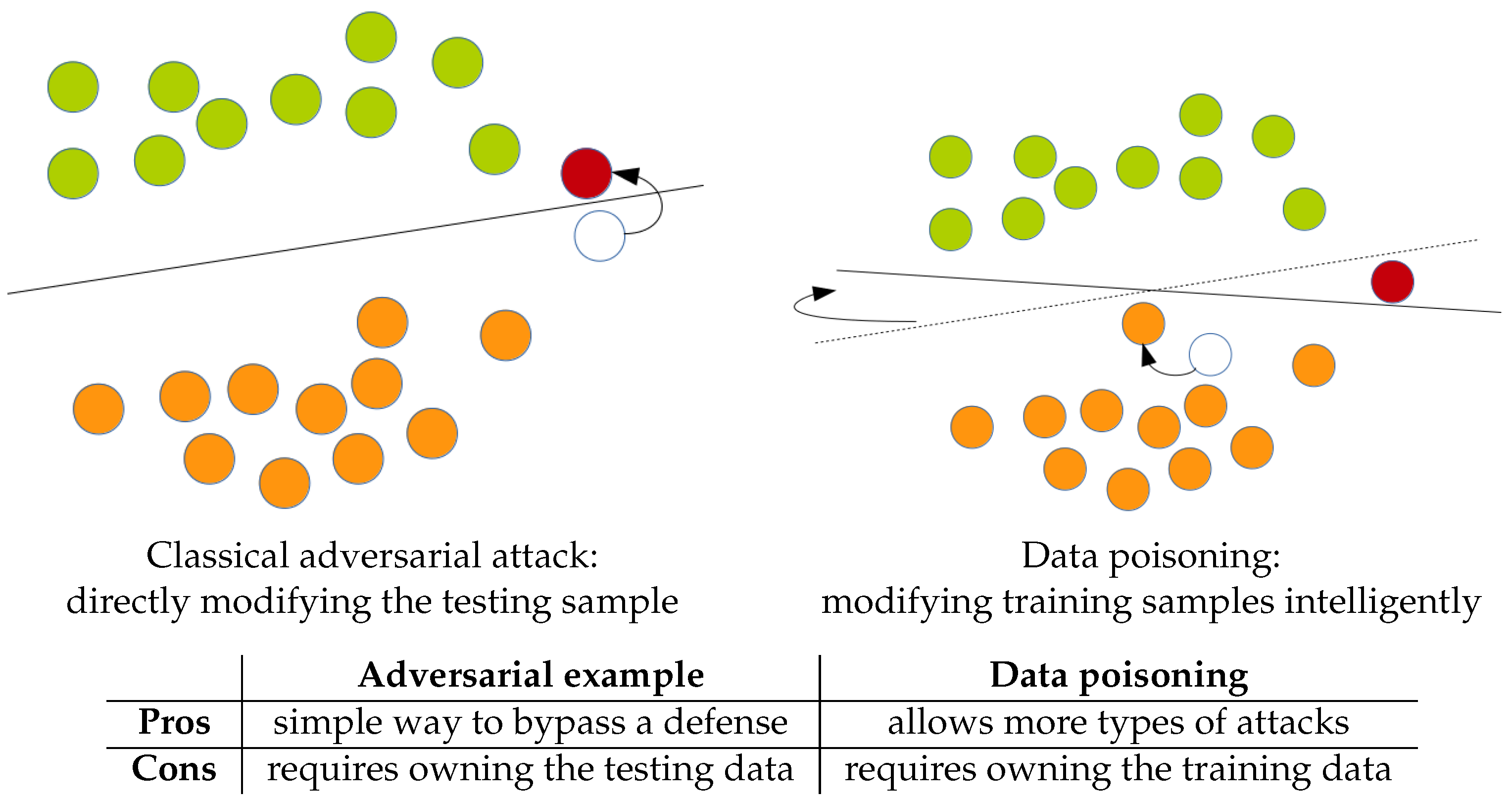
4.5. Comparison with Classical Adversarial Attack

Let me recall the difference between the classical adversarial attack and adversarial-based data poisoning (see also Figure 3):

• An adversarial attack is a small modification of the testing samples to break the testing accuracy
• Adversarial-based data poisoning is a small modification of the training samples that breaks the testing accuracy after training on the poisoned training data

For providing more support to the discussion, Algorithm 1 compares the accuracy loss under both settings. The classical adversarial is implemented under a white-box setting, but results should be similar to [13]. The main result is that adversarial poisoning and classical adversarial attacks attain similar accuracy gaps. Yet, as the requirements are different, the two types of attack are not directly comparable. Indeed, even if less straightforward than the classical adversarial attack, data poisoning enables an attack when the testing data are not owned by the hacker (but known).

In addition, it is also possible to compare these performances to the one reached by the pipeline when trained on fair adversarial (in opposition to adversarial-based poisoning). Specifically, training on fair adversarial corresponds to using $-{\theta }^{fair}$ instead of ${\theta }^{poison}$. However, this changes everything. Adding adversarial to the training set is even a classical way to increase network robustness [18]. Moreover, this is not a hack—this is just a step in the training process (no knowledge from the test is imported). So, there is no reason that such a process will break the testing accuracy (it could improve it by reducing overfitting). Indeed,

Table 1. Comparison of accuracy loss between the adversarial attack and data poisoning on CIFAR.

Accuracy Loss	Data Poisoning	Classical Adversarial	Adversarial Training
vs Dataset	(Hacking Train)	(Hacking Test)	(Updated Training)
CIFAR10	−12%	−18%	0%
CIFAR100	−13%	−15%	−2%

shows that training on fair adversarial does not change the testing accuracy.

This last point shows the importance of the introduction of the desired weights which capture information on the testing set (remember, this paper deals with the hacking context). Without these weights, training sample modification can result in zero accuracy loss at testing time.

4.6. Inverse Poisoning

Here, inverse poisoning is considered to provide another point to the discussion.

As the return favor algorithm works with desired weights ${\theta }^{poison}$, it is possible to use other weights for goals other than accuracy minimization. For example, it is possible to use weights which have a very high accuracy instead of a very low one.

When applying the return favor algorithm one time using the entire dataset with desired weights opposite to that in Section 4.3, the performance jumps to an 82% accuracy on CIFAR10 and a 66% accuracy on CIFAR100. When applying it three times, the performances explode to reach a 92% accuracy on CIFAR10 and a 78% accuracy on CIFAR100, which are better than the fair state-of-the-art (see https://benchmarks.ai/cifar-100)! This is not surprising, as the desired weights contain knowledge from the testing set. However, this result shows the strong impact of the noise computed by the proposed algorithm: the accuracy gap corresponds to 3 years of research on CIFAR. This can add some elements of comparison to the state-of-the-art, as the direct comparison of different poisonings for this paper was not easy.

5. Conclusions

This paper introduces a new kind of data poisoning: invisible data poisoning. This attack aims to pervert a learning system thanks to a low-amplitude perturbation of the training samples, contrary to classical poisoning which relies on a perturbation of a low number of samples. The main contribution of this paper is the successful implementation of such invisible data poisoning of deep learning using publicly available image datasets. This implementation takes advantage of algorithms originally designed for adversarial examples. Our experiments show that such attacks can have critical effects: on CIFAR100, the poisoning leads to an accuracy gap of nearly 30% while being invisible to human eyes.

Seeing these results, the community should be mindful of the threat of classical data poisoning, but also be aware of the risk of invisible data poisoning.

References

1. Krizhevsky, A.; Sutskever, I.; Hinton, G.E. Imagenet Classification with Deep Convolutional Neural Networks. In Advances in Neural Information Processing Systems; 2012; pp. 1097–1105. [Google Scholar]
2. LeCun, Y.; Bengio, Y.; Hinton, G. Deep learning. Nature 2015, 521, 436–444. [Google Scholar] [CrossRef] [PubMed]
3. Taigman, Y.; Yang, M.; Ranzato, M.; Wolf, L. Deepface: Closing the Gap to Human-Level Performance in Face Verification. In Proceedings of the IEEE Conference on Computer Vision and Pattern Recognition, Columbus, OH, USA, 24–27 June 2014; pp. 1701–1708. [Google Scholar]
4. Cordts, M.; Omran, M.; Ramos, S.; Rehfeld, T.; Enzweiler, M.; Benenson, R.; Franke, U.; Roth, S.; Schiele, B. The Cityscapes Dataset for Semantic Urban Scene Understanding. In Proceedings of the Conference on Computer Vision and Pattern Recognition, Las Vegas, NV, USA, 27–30 June 2016; pp. 3213–3223. [Google Scholar]
5. Greenspan, H.; van Ginneken, B.; Summers, R.M. Guest Editorial Deep Learning in Medical Imaging: Overview and Future Promise of an Exciting New Technique. IEEE Trans. Med. Imagingg 2016, 35, 1153–1159. [Google Scholar] [CrossRef] [Green Version]
6. Alsulami, B.; Dauber, E.; Harang, R.; Mancoridis, S.; Greenstadt, R. Source Code Authorship Attribution Using Long Short-Term Memory Based Networks. In European Symposium on Research in Computer Security; Springer: Cham, Germany, 2017; pp. 65–82. [Google Scholar]
7. Javaid, A.; Niyaz, Q.; Sun, W.; Alam, M. A Deep Learning Approach for Network Intrusion Detection System. In Proceedings of the 9th EAI International Conference on Bio-inspired Information and Communications Technologies (formerly BIONETICS); 2016; pp. 21–26. [Google Scholar]
8. Moosavi Dezfooli, S.M.; Fawzi, A.; Fawzi, O.; Frossard, P. Universal Adversarial Perturbations. In Proceedings of the IEEE Conference on Computer Vision and Pattern Recognition (CVPR), Honolulu, HI, USA, 21–26 July 2017. [Google Scholar]
9. Xie, C.; Wang, J.; Zhang, Z.; Zhou, Y.; Xie, L.; Yuille, A. Adversarial Examples for Semantic Segmentation and Object Detection. In Proceedings of the IEEE International Conference on Computer Vision (ICCV), Venice, Italy, 22–29 October 2017. [Google Scholar]
10. Papernot, N.; McDaniel, P.; Jha, S.; Fredrikson, M.; Celik, Z.B.; Swami, A. The Limitations of Deep Learning in Adversarial Settings. In Proceedings of the 2016 IEEE European Symposium on Security and Privacy (EuroS&P), Saarbrucken, Germany, 21–24 March 2016; pp. 372–387. [Google Scholar]
11. Szegedy, C.; Zaremba, W.; Sutskever, I.; Bruna, J.; Erhan, D.; Goodfellow, I.J.; Fergus, R. Intriguing Properties of Neural Networks. arXiv, 2013; arXiv:1312.6199. [Google Scholar]
12. Grosse, K.; Papernot, N.; Manoharan, P.; Backes, M.; McDaniel, P. Adversarial Examples for Malware Detection. In European Symposium on Research in Computer Security; Springer: Cham, Germany, 2017; pp. 62–79. [Google Scholar]
13. Cisse, M.M.; Adi, Y.; Neverova, N.; Keshet, J. Houdini: Fooling Deep Structured Visual and Speech Recognition Models with Adversarial Examples. In Advances in Neural Information Processing Systems; MIT Press: Cambridge, MA, USA, 2017; pp. 6977–6987. [Google Scholar]
14. Narodytska, N.; Kasiviswanathan, S. Simple Black-Box Adversarial Attacks on Deep Neural Networks. In Proceedings of the IEEE Conference on Computer Vision and Pattern Recognition Workshops (CVPRW), Honolulu, HI, USA, 21–26 July 2017; pp. 6–14. [Google Scholar]
15. Zhang, C.; Bengio, S.; Hardt, M.; Recht, B.; Vinyals, O. Understanding Deep Learning Requires Rethinking Generalization. arXiv, 2016; arXiv:1611.03530. [Google Scholar]
16. Kurakin, A.; Goodfellow, I.J.; Bengio, S. Adversarial Examples in the Physical World. arXiv, 2016; arXiv:1607.02533. [Google Scholar]
17. Liu, L.; De Vel, O.; Han, Q.L.; Zhang, J.; Xiang, Y. Detecting and Preventing Cyber Insider Threats: A Survey. IEEE Commun. Surv. Tutor. 2018, 20, 1397–1417. [Google Scholar] [CrossRef]
18. Muñoz-González, L.; Biggio, B.; Demontis, A.; Paudice, A.; Wongrassamee, V.; Lupu, E.C.; Roli, F. Towards Poisoning of Deep Learning Algorithms with Back-Gradient Optimization. In Proceedings of the 10th ACM Workshop on Artificial Intelligence and Security; ACM: New York, NY, USA, 2017; pp. 27–38. [Google Scholar]
19. Krizhevsky, A.; Hinton, G.E. Using very Deep Autoencoders for Content-Based Image Retrieval. In Proceedings of the 19th European Symposium on Artificial Neural Networks, Bruges, Belgium, 27–29 April 2011. [Google Scholar]
20. Vapnik, V.N.; Vapnik, V. Statistical Learning Theory; Wiley: New York, NY, USA, 1998; Volume 1. [Google Scholar]
21. LeCun, Y.; Boser, B.E.; Denker, J.S.; Henderson, D.; Howard, R.E.; Hubbard, W.E.; Jackel, L.D. Handwritten Digit Recognition with a Back-Propagation Network. In Advances in Neural Information Processing Systems; MIT Press: Cambridge, MA, USA, 1990; pp. 396–404. [Google Scholar]
22. Fischler, M.A.; Bolles, R.C. Random sample consensus: a paradigm for model fitting with applications to image analysis and automated cartography. In Readings in Computer Vision; Elsevier: Amsterdam, The Netherlands, 1987; pp. 726–740. [Google Scholar]
23. Liu, S.; Zhang, J.; Wang, Y.; Zhou, W.; Xiang, Y.; Vel., O.D. A Data-driven Attack Against Support Vectors of SVM. In Proceedings of the 2018 on Asia Conference on Computer and Communications Security; ASIACCS ’18; ACM: New York, NY, USA, 2018; pp. 723–734. [Google Scholar] [CrossRef]
24. Girshick, R.; Donahue, J.; Darrell, T.; Malik, J. Rich Feature Hierarchies for Accurate Object Detection and Semantic Segmentation. In Proceedings of the IEEE Conference on Computer Vision and Pattern Recognition (CVPR), Columbus, OH, USA, 24–27 June 2014; pp. 580–587. [Google Scholar]
25. Deng, J.; Dong, W.; Socher, R.; Li, L.J.; Li, K.; Fei-Fei, L. Imagenet: A large-scale hierarchical image database. In Proceedings of the 2009 IEEE Computer Society Conference on Computer Vision and Pattern Recognition (CVPR 2009), Miami, FL, USA, 20–25 June 2009; pp. 248–255. [Google Scholar]
26. Fan, R.E.; Chang, K.W.; Hsieh, C.J.; Wang, X.R.; Lin, C.J. LIBLINEAR: A Library for Large Linear Classification. J. Mach. Learn. Res. 2008, 9, 1871–1874. [Google Scholar]
Figure 1. Adding uniform random noise to all pixel values. This figure just shows how it is difficult for a human to perceive a small modification in an image: here, this sequences of images is formed by adding uniform noise of amplitudes of 0, 5, 10, ..., 40 units (coded from 0 to 255) to each pixel value of the original image.
Make 01 00011 g001
Figure 2. Samples of the original, difference, and poisoned images. This figure presents some original (left) vs poisoned images (right) and the difference averaged over the three channels and scaled 80 times. Deformation is either +1 or −1 for each channel of each pixel. Blue corresponds to negative transformations and green indicates positive ones.
Make 01 00011 g002
Figure 3. Illustrations of adversarial examples and adversarial-based data poisoning. The red point is a testing sample with the same classes as the orange ones. The goal of attacks is to have it classified as green.
Make 01 00011 g003