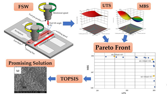
Multi-Objective Variable Neighborhood Strategy Adaptive Search for Tuning Optimal Parameters of SSM-ADC12 Aluminum Friction Stir Welding

Abstract

This research presents a novel algorithm for finding the most promising parameters of friction stir welding to maximize the ultimate tensile strength (UTS) and maximum bending strength (MBS) of a butt joint made of the semi-solid material (SSM) ADC12 aluminum. The relevant welding parameters are rotational speed, welding speed, tool tilt, tool pin profile, and rotation. We used the multi-objective variable neighborhood strategy adaptive search (MOVaNSAS) to find the optimal parameters. We employed the D-optimal to find the regression model to predict for both objectives subjected to the given range of parameters. Afterward, we used MOVaNSAS to find the Pareto front of the objective functions, and TOPSIS to find the most promising set of parameters. The computational results show that the UTS and MBS of MOVaNSAS generate a 2.13% to 10.27% better solution than those of the genetic algorithm (GA), differential evolution algorithm (DE), and D-optimal solution. The optimal parameters obtained from MOVaNSAS were a rotation speed of 1469.44 rpm, a welding speed of 80.35 mm/min, a tool tilt of 1.01°, a cylindrical tool pin profile, and a clockwise rotational direction.

1. Introduction

Cast aluminum has been used in innovative creations such as auto engines, turbine engines, etc., because it has good mechanical properties and easy fabrication. However, the problems with cast aluminum are defects in the structure such as porosity, cracking, and different gains that are difficult to control when cooling down after the casting process. Therefore, cast aluminum use has been reduced in auto engines and turbine engines. SSM (semi-solid material) aluminum was generated to compensate for the problems of cast aluminum because SSM aluminum is fabricated by a process that controls the different gains and defects within the structure. Therefore, semi-solid metal aluminum has been widely used in engine parts in aerospace, automobile, and marine products. The welding process is important to the engine part joint. Fusion welding has been the conventional way of metal welding, but it is a difficult process for aluminum welding. As aluminum material has a low melting point, the fusion welding process generates too high heat for welding. After welding, the welded seam temperature is reduced rapidly by ambient air that affects welded seam through cracking, porosity, distortion, and different gains [1,2,3,4].

Solid-state welding joints are used to reduce problems of distortion, cracking, and metallurgical changing. Friction stir welding (FSW) generates welding temperatures lower than the melting point temperature of materials, resulting in less gain changing and favorable joints after material welding [5,6,7,8,9,10]. Therefore, the friction stir welding process produces a welded seam with sufficient mechanical properties and structure [11,12]. Several works have studied the relative process parameters of mechanical properties and metallurgical structure. The parameters measure influences on welded seam quality, including rotation speed, welding speed, tilt angle, tool geometries, and the ratio shoulder to pin diameter (D/d), that affect heat generation, material deformation, material flow, material mixing, defects, strength, and metallurgical changing in weld line structure [13,14,15,16,17,18,19]. The parameters of the friction stir welding process have been studied by optimized methods such as factorial design [20], Taguchi design [21,22], grey relational method [23,24], response surface method [13,25], and combined methods [26,27,28,29]. The optimized methods can effectively control the mechanical property and defects of the weld line [30,31,32]. The weld line performance depends on many properties, such as tensile strength, hardness, impact, corrosion resistance, etc. A survey of the literature found that several kinds of research have emphasized that the main property target is tensile strength, in that it affects weld line usability performance. Consequently, tensile testing is used for quality measurements of weld line structures, being the main performance indicator of materials [33]. Thus, tensile strength has not been neglected in considering the mechanical property of the weld line. The hardness property is the second mechanical property of interest to study. Both hardness and tensile properties have a direct relationship with the material’s exhibited high hardness value, and the tensile strength will increase in value, according to the reports of Khodabakhshi and Gerlich [34], and Chen and Cai [35]. Thus, hardness and other mechanical properties are ignored in the many studies shown in

Table 1. Prediction approaches and response optimization from literature reviews.

Authors	Experimental Design Approach	Predicted Approaches	Optimized Multi-Responses	Method Error (%)
This work	D-optimal	VaNSAS, Pareto Frontier and TOPSIS	Tension and Bending
Senthil et al. (2020) [37]	RSM	ANOVA	Elongation and Tension	3.7
Sharma et al. (2019) [39]	Taguchi	GRA and TOPSIS	Tension and Hardness	3.43
Goyal and Garg (2018) [40]	RSM	ANOVA	Tension and Hardness	2.6
Wakchaure et al. (2018) [29]	Taguchi	GRA and ANN	Tension and impact	3.25
Kamal Babu et al. (2017) [41]	Taguchi	ANN and GA	Tension, Hardness, and Corrosion	2.27
Tamjidy et al. (2017) [42]	RSM	Pareto Frontier, TOPSIS and Shannon	Elongation, Tension, and Hardness	0.59
Kumar Gupta et al. (2016) [38]	Taguchi	GRA	Grain size, Tension, and Hardness	15.42
Kesharwani et al. (2014) [43]	Taguchi	GRA	Elongation and Tension	11.25
Roshan et al. (2013) [44]	RSM	ANFIS and SA	Tension and Hardness	2.24

RSM = Response surface method, FEM = Finite element method, ANN = Artificial neural network, SA = Simulated annealing algorithm, ANFIS = Adaptive neuro-fuzzy inference systems, GRA = Grey relation analysis, GA = Genetic algorithm, VaNSAS = Variable neighborhood strategy adaptive search, TOPSIS = Technique for order of preference by similarity to ideal solution, ANOVA = Analysis of variance.

. Moreover, the mechanical property study of weld seams depends on weld line usability. However, bending is the weld line mechanical property that has not been studied for quality improvement in the automotive or marine industries. Therefore, the bending property should be studied together with the other properties. Several studies on aluminum alloy welding have presented optimization of the multi-objective strategy for many properties together in one welding condition because it provides desirable property parameters for the target requirement [29,36,37,38].

However, although the optimized method gives prediction results for target satisfaction, it shows a high error percentage average between 2% and 15% [38,39,44]. Improvement of the optimized method is important for response prediction accuracy. Furthermore, this approach to optimized parameter finding was developed based on the heuristic approach. Optimization predictions in many studies have used heuristic methods for problem solving that displayed accurate success and fast response times. Several heuristic approaches displayed high effectiveness, such as the technique for order of preference by similarity to ideal solution (TOPSIS), differential evolution algorithms (DEs), artificial neural networks (ANNs), genetic algorithms (GAs), adaptive large neighborhood search (ALNS), etc., and these methods have been used to optimize tour routing, transportation, agriculture, welding, and manufacturing processes [39,45,46,47,48,49,50,51]. The optimization finding for welding conditions is especially important because inappropriate welding conditions deteriorate the quality of the weld line. Therefore, the heuristic approach is used as an optimized parameter in the FSW process because the result of the optimized welding parameter exhibited a low range error of approach of 0.5–3% [30,42,45,52], as shown in Table 1. The heuristic approach is highly effective for optimized parameter prediction. Moreover, the Pareto optimization is used for optimal parameter finding together with a heuristic approach. This increases the exactness of optimal parameter prediction, especially in multi-objective optimization [29,37,43].

Therefore, in this work, we present the variable neighborhood strategy adaptive search (VaNSAS) and Pareto optimal for finding the optimal parameters in the FSW process. The welding feature is the butt joint for SSM ADC 12 aluminum material. The welding optimization parameters are rotation speed, welding speed, tool tilt angle, and tool geometry. The two optimization responses are the tensile and bending strengths of the weld line. The weld line structure is studied by scanning electron microscope (SEM) to determine the weldability characteristics and defects.

2. Literature Survey

The FSW process has several important parameters, but we found that two parameters mainly affect weld joint performance, namely, rotation speed and welding speed. These parameters indicate the heat generation deformation of the material and material flow in welding [12,52,53,54], so that both the rotation speed and welding speed parameters cannot be ignored in the FSW process. Other parameters that are supported to improve the weld joint quality are tilt angle, tool geometries, the ratio of shoulder to pin diameter (D/d), and tool material. Some FSW cases could be omitted in advocated parameter studies, but the weld line quality gives a highly effective performance, as shown in Table 2. Nevertheless, these advocated parameters are given importance to increase the weld line performance. Both tilt angle and tool geometries are especially influential parameters for effective material flow when fulfilling and mixing the material within the weld joint, which decreased or eliminated defects in the structure [55,56,57,58,59].

For the parameters of the ratio of shoulder to pin diameter (D/d) and the axial force affected by the heat generation and process force in the initial welding, the influence of two parameters was reduced for weld line creation [60,61,62]. However, the tool loading force showed a significant effect on the initial welding. The tool loading force parameter expedited high heat generation for the plastic deformation of the material and reduced axial force after material deformation. The tool loading force parameter does not affect the weld movement [63] because the heat in the welding process is controlled by two parameters, rotation speed and welding speed. Therefore, the tool axial force parameter has been ignored in many previous studies, as shown in Table 2.

Table 2. Parameters study for optimization from literature reviews.

Authors	Approaches for Optimization	Material Joint		Materials		Study Parameters
		Similar	Dissimilar		Rotation Speed	Welding Speed	Tilt Angle	Tool Geometry	D/d Ratio	Axial Force	Tool Material	Tool Offset	Rotational Direction
This work	D-optimal and VaNSAS	✔		SSM-ADC12	✔	✔	✔	✔					✔
Meengam and Sillapasa (2020) [20]	Factorial design	✔		SSM-Al 6063	✔	✔		✔
Senthil et al. (2020) [37]	RSM	✔		AA 6063	✔	✔
Shanavas and Dhas (2017) [25]	RSM	✔		AA 5052	✔	✔	✔	✔
Ghaffarpour et al. (2015) [64]	RSM		✔	AA 5083-AA 6061	✔	✔	✔		✔
Kumar Gupta et al. (2016) [38]	Taguchi and GRA		✔	AA 5083-AA 6063	✔	✔			✔
Kesharwani et al. (2014) [43]	Taguchi and GRA		✔	AA5052-AA5754	✔	✔		✔	✔
Shaik et al. (2019) [32]	Taguchi and GRA		✔	AA6082-AA7075	✔	✔	✔
Wakchaure et al. (2018) [29]	GRA and ANN	✔		AA6082	✔	✔	✔	✔
Siva et al. (2019) [65]	GRA and TOPSIS	✔		NAB alloy	✔	✔				✔
Kamal Babu et al. (2017) [41]	ANN and GA	✔		AA2219	✔	✔	✔
Sharma et al. (2019) [39]	Taguchi and TOPSIS		✔	AA6101-Copper	✔	✔			✔			✔
Shojaeefard et al. (2013) [28]	ANN and PSO		✔	AA7075-AA5083	✔	✔
Tamjidy et al. (2017) [42]	TOPSIS and Shannon’s entropy		✔	AA 6061-AA7075	✔	✔	✔					✔
Roshan et al. (2013) [44]	ANFIS and SA	✔		AA7075	✔	✔		✔		✔
Shojaeefard et al. (2014) [36]	FEM and ANN	✔		AA 5083	✔	✔

Table 2. Parameters study for optimization from literature reviews.

Authors	Approaches for Optimization	Material Joint		Materials		Study Parameters
		Similar	Dissimilar		Rotation Speed	Welding Speed	Tilt Angle	Tool Geometry	D/d Ratio	Axial Force	Tool Material	Tool Offset	Rotational Direction
This work	D-optimal and VaNSAS	✔		SSM-ADC12	✔	✔	✔	✔					✔
Meengam and Sillapasa (2020) [20]	Factorial design	✔		SSM-Al 6063	✔	✔		✔
Senthil et al. (2020) [37]	RSM	✔		AA 6063	✔	✔
Shanavas and Dhas (2017) [25]	RSM	✔		AA 5052	✔	✔	✔	✔
Ghaffarpour et al. (2015) [64]	RSM		✔	AA 5083-AA 6061	✔	✔	✔		✔
Kumar Gupta et al. (2016) [38]	Taguchi and GRA		✔	AA 5083-AA 6063	✔	✔			✔
Kesharwani et al. (2014) [43]	Taguchi and GRA		✔	AA5052-AA5754	✔	✔		✔	✔
Shaik et al. (2019) [32]	Taguchi and GRA		✔	AA6082-AA7075	✔	✔	✔
Wakchaure et al. (2018) [29]	GRA and ANN	✔		AA6082	✔	✔	✔	✔
Siva et al. (2019) [65]	GRA and TOPSIS	✔		NAB alloy	✔	✔				✔
Kamal Babu et al. (2017) [41]	ANN and GA	✔		AA2219	✔	✔	✔
Sharma et al. (2019) [39]	Taguchi and TOPSIS		✔	AA6101-Copper	✔	✔			✔			✔
Shojaeefard et al. (2013) [28]	ANN and PSO		✔	AA7075-AA5083	✔	✔
Tamjidy et al. (2017) [42]	TOPSIS and Shannon’s entropy		✔	AA 6061-AA7075	✔	✔	✔					✔
Roshan et al. (2013) [44]	ANFIS and SA	✔		AA7075	✔	✔		✔		✔
Shojaeefard et al. (2014) [36]	FEM and ANN	✔		AA 5083	✔	✔

The tool material was a low effect parameter of whether material hardness selection was suited to the material type of the workpiece. The weld joint was unaffected by tool material [66,67]. The literature review emphasized the two main parameters, namely, rotation speed and welding speed of FSW, that affected heat generation deformation and microstructure changing. The other parameter was secondary in that it could help to improve avocation of the weld line quality and decrease defects in the structure. Therefore, parameter selection for studies on FSW depended on consideration of the consequences of the parameter, such that much research on the effects of welding parameter control was carried out with diverse approaches to many responses. Several experimental design methods for optimized parameters were used, such as factorial design, response surface method, Taguchi design, and D-optimal. Each experimental design method showed differences in the number of experiments and design steps that depended on the number of parameters and level values. However, when comparing the experimental design methods with many mixed levels from similar factor numbers, the D-optimal design approach exhibited a low number of experiments and many level values of parameters [68,69,70]. Thus, D-optimal design was used as an experimental design in much research.

Many optimal approaches to finding parameters of the welding process were used to predict the response to the development of the weld line quality. The local search approach was often used to optimize parameter conditions owing to its uncomplicated and desirable results. In 2020, Senthil et al. [37] presented the response surface method for optimization of the FSW parameters of aluminum pipe. Two welding parameters were rotation speed and welding speed, which was a main parameter of FSW. The two types of mechanical property objectives for optimization were tensile strength and elongation percentage, which was multi-objective in one condition. The optimized condition for FSW displayed improvement in the two properties to increase tensile strength and suitable elongation percentage. The error of the prediction method was 3.7% when compared with the confirmed result. Accordingly, Goyal and Garg [40] and Shanavas and Dhas [25] used the RSM method and ANOVA approach to find optimal parameter conditions of marine-grade aluminum. The focus of the study was tensile strength elongation percentage and hardness of the weld line. This method showed high effectiveness of result prediction because it indicated an improvement in the mechanical property and desired quality of weld line usability. In addition, the Taguchi design was used for experimental design and optimal parameter conditions with grey relation analysis (GRA) or analysis of variance (ANOVA) in FSW. Ramesha et al. [53] and Prasad and Namala [71] used the Taguchi design and ANOVA approach for multi-objective optimization of dissimilar aluminum welding. Both tensile strength and hardness were used for one optimal parameter prediction. The result of the optimal parameter displayed high weld joint performance of the properties of tensile strength and hardness together. Although the optimum welding condition showed good mechanical property of the weld line, a tunnel defect appeared in the structure. Therefore, the GRA approach was developed to increase the effectiveness of the optimized parameter prediction method and reduce defects in the structure, which offered a good solution and reduced defects in the weld joint. Shaik et al. [32] studied multi-objective optimization on three properties, namely, tensile, elongation, and impact of the weld joint. The Taguchi design and GRA approach were used to design an experiment and optimal parameter condition prediction. The weld line of optimal parameter welding conditions exhibited a satisfying performance and no defect in the weld joint. However, the effectiveness of the prediction approach gave a high prediction error when comparing the result confirmation, ranging from 11–15%, as reported by Gupta et al. [38] and Kesharwani et al. [43].

The heuristic approach was used to develop the solution prediction method of the FSW process. Sharma et al. [39] presented the Taguchi design and TOPSIS approach to find the optimal parameter in a multi-objective response. The performance prediction for the weld joint showed increased accuracy in the multi-response of one optimal welding parameter that reduced the method error to 3.42%. Accordingly, Siva et al. [65] used the Taguchi experimental design and combined both GRA and TOPSIS in their improvement of the optimal welding parameters in multi-response. The prediction method showed satisfactory results and effectively controlled defects of the weld seam. Wakchaure et al. [29] presented the combined method of GRA and an artificial neural network (ANN) for optimized welding parameters of tensile strength and impact. The error of the prediction process was 3.25% of the confirmed result, and the weld line displayed high effective strength. The heuristic method of an ANN and genetic algorithm (GA) was used to optimize welding process conditions of mechanical and corrosion properties in cryorolled aluminum welding. The experiment followed the Taguchi design approach for collection of mechanical and corrosion response data. After that, the experiment data were used for the optimized prediction of the parameter process. The weld joint showed high effective mechanical and corrosion properties with an optimized welding parameter that was presented by Babu et al. [41]. However, the prediction method error was not acceptable because it was high when compared to the confirmed result. Tamjidy et al. [42] presented the prediction development for FSW using a biogeography-based optimization algorithm, including the Pareto optimal frontier approach for optimal result selection and TOPSIS and Shannon’s entropy approach for decision making in solution accepting. The Pareto optimal approach offered the choice of several optimal solution predictions, which contained too many values for the desire response. However, the several optimal results could not satisfy decision making for the determinative target. The heuristic approach of TOPSIS and Shannon’s entropy selected the best optimal solution in the group, resulting in a low error of 0.59%. Accordingly, Shojaeefard et al. [28] used the Pareto optimal frontiers method together with other heuristic methods in FSW, which provided highly effective optimal solution generation for multi-objective response.

Therefore, development of the heuristic method is important for decreasing error prediction. An accuracy prediction method depends on the characteristics of the heuristic algorithm. Several approach generations in one heuristic algorithm have displayed the high infallibility of the prediction method. One heuristic algorithm has exhibited very accurate solution finding, namely, the variable neighborhood strategy adaptive search (VaNSAS) approach. The VaNSAS algorithm has shown prominent solution finding on several algorithms in the improvement box. Therefore, the precision of the VaNSAS algorithm has been demonstrated by several researchers. Jirasirilerd et al. [45], Pitakaso et al. [51], and Pitakaso et al. [50] studied problem solving in production and planning with the VaNSAS algorithm. The improvement box operations to process the VaNSAS algorithm were the differential evolution algorithm, iterated local search, swap method, modified differential evolution algorithm, large neighborhood search, and shortest processing time-swap. The prediction accuracy result of the VaNSAS algorithm showed a high precision up to 99.99%, such that the error rate was 0.01% for predicted solutions. Therefore, the VaNSAS algorithm is a high accuracy approach and offers excellent result prediction. In this paper, the VaNSAS is firstly extended for use with the multi-objective decision making. The main mechanism of VaNSAS remains the same when it is applied to solving the multi-objective problem. The general procedure of VaNSAS is composed of four steps: (1) generate the initial set of solutions; (2) perform the track touring process; (3) update the heuristics information, and (4) re-do steps (2) and (3) until a termination condition is met. In the track touring process, the best solution will survive to tour in the next iteration. The weighted sum method is used to select the survival track to use in the next iteration. Then, the Pareto front is collected during the simulation, and TOPSIS is used to select the promising solution The multi-objective variable neighborhood strategy adaptive search is called MOVaNSAS.

3. Materials and Methods

The general steps in our proposed method include (1) identifying the number, types, and levels of the interested parameters from a literature survey and using the D-optimal experimental design to reveal the regression model to predict the target parameters for friction stir welding; (2) using MOVaNSAS to find the optimal set of parameters; and (3) performing an experiment to confirm the result obtained from (2), which is explained stepwise in the following subsection.

3.1. Identifying the Number, Types, and Levels of the Interested Parameters Using D-Optimal Experimental Design to Find the Regression Model to Predict the Target Parameters for Friction Stir Welding

Table 3. Chemical properties of base ADC12.

	Chemical Composition
	Al	Cu	Mg	Fe	Sn	Ni	Zn	Mn	Si	Other
(SSM) ADC12	Bal.	2.0–3.0	0.1	1.3	0.15	0.3	3.0	0.5	9.5–11.5	0.5

shows the chemical composition of the workpiece used in our experiment. The previous research is shown in Table 1 and Table 2, and the target parameter types and levels used in this research are shown in

Table 4. Parameters in the experiment.

Continuous variable
Parameter	Levels
	−1	1
Rotation speed (rpm), S	1100	2200
Welding speed (mm/min), F	80	200
Tool tilt angle (Deg.), T	0	6
Categorical variables
Parameter	Levels
Tool pin profile	Cylindrical	Hexagon
Rotational direction	Clockwise: CW	Counterclockwise: CCW

.

The interested parameter types were separated into two groups: (1) continuous and (2) categorical. Each continuous parameter shows a value between code −1 and 1, as shown in Table 4. There were three continuous variables: (1) rotational speed, 1100–2200 rpm (S); (2) welding speed, 80–200 mm/min (F); and (3) tool tilt angle, 0°–6° (T). The two categorical variables were set as (1) tool pin profiles of cylindrical shape and hexagon shape and (2) different tool rotations of clockwise and counterclockwise directions.

The experiments were carried out according to a D-optimal experimental design (D-opt). D-opt was used to select h design points from value sets of each interested parameters by the embedding algorithm, resulting in 19 minimum model points, 5 points for estimation of the lack-of-fit, and 5 points for replicates. Finally, an experimental plan with a total of 29 points was created.

The upper and lower limits of the parameters in the statistical software Design-Expert (Stat-Ease, Inc., Minneapolis, MN, USA) were set to −1 and 1.

The intermediate coded values were calculated using Equation (1):

$$Original=\frac{Scaled \left[\left(X_{Max}+X_{min}\right)\right]+X_{Max}+X_{min}}{2}$$

(1)

where $Scaled$ is the required coded value of a variable X; X is any value of the variable from $X_{min }$ to $X_{Max}$; and $X_{min}$ and $X_{Max}$ are the lowest and highest predefined values of the parameter, respectively. Table 4 provides the details of each uncoded parameter, which includes the upper and lower bounds of these parameters.

D-optimal software was used to design and create the experimental models and problem analysis. The quadratic model shown in Equation (2) is obtained from the experiment:

$$y=b_0+{\displaystyle \sum _i^k}{b}_i{x}_i+{\displaystyle \sum _i^k}{b}_{ii}{x}_i^2+{\displaystyle \sum _i}{\displaystyle \sum _j}{b}_{ij}{x}_i{x}_j+\epsilon$$

(2)

where $y$ is the ultimate tensile strength (response), $x_i$ is the uncoded levels of the variables, $\epsilon$ is the fitting error, the coefficient $b_0$ is the constant value or intercept and coefficients, and $b_i$, $b_{ii},$ and $b_{ij}$ represent the linear, quadratic, and interaction terms of the variables, respectively [72].

3.2. Using the Multi-Objective Variable Neighborhood Strategy Adaptive Search (MOVaNSAS) to Find the Optimal Parameters

The multi-objective variable neighborhood strategy adaptive search (MOVaNSAS) approach is a new metaheuristic to search for a solution in a large searching area. Several approaches are gathered into one method in an improvement box to search for the best solution. MOVaNSAS is composed of four steps [45], as follows.

3.2.1. Generate a Set of Initial Tracks

The initial set of tracks is the real number that is uniformly randomly generated from Equation (3).

$$Y_{ij1}=U\left(0,1\right)$$

(3)

where $Y_{ij1}$ is the value in track i, position j at iteration 1. j is the number of interest parameters, i is the number of tracks, which is a predefined number. $Y_{ijt}$ is decoded as the value of rotational speed, welding speed, tool tilt angle, tool pin profile, and rotational direction using Equation (4).

$$R=L+e\left(U-L\right)$$

(4)

where $R$ is value of the parameter, L is the lowest allowed value of the parameter, U is the highest allowed value of the parameter, and $e$ is the value in position ($Y_{ijt})$. For example, if $Y_{111}$(rotation speed) is 0.36, the value of the real rotation speed is 1100 + [(0.36) × (2200 − 1100)] = 1496. The next step of MOVaNSAS is the track touring process, which is explained as follows.

3.2.2. Perform Track Touring Process (TTP) in a Specified Improvement Box

MOVaNSAS will use the track touring process to improve the current solution quality. In the track touring process, all tracks will independently select an improvement box to improve their quality. The improvement boxes used in this section are: (1) differential equation method (DEM), (2) best track transition method (B-TTM), track transition method (TTM), and random track transition method (R-TTM). The roulette wheel selection is used to select the improvement box with specified probability function Equation (5).

$$P_{bt}=\frac{F{N}_{bt-1}+\left(1-F\right)A_{bt-1}+K{I}_{bt-1}}{{\sum }_{bt=1}^n{W}_{bt}}$$

(5)

where P_bt is the probability of the selection of an improvement box in iteration t; N_bt−1 is the number of tracks that selected an improvement box in the previous iteration; A_bt−1 is the average objective value of all tracks that selected an improvement box in the previous iteration; and I_bt−1 is a reward value, increased by 1 if an improvement box finds the best solution in the last iteration, but set to 0 if this is not the case. Additionally, W_bt is the weight of the improvement box, F is the scaling factor, which is set to 0.5, and K is the parameter factor, which is set to 0.3 [45]. The improvement boxes are revealed in the next section.

• Improvement Box Operation

The improvement box operation step allows finding a solution from three selected approaches in each improvement box. These are as follows:

• Differential Equation Method (DEM)

This method employs the basic idea of the differential evolution algorithm. The update of $Y_{ijt}$ can be executed by Equation (6).

$$Y_{ijq}=Y_{rjq}+F\left(Y_{mjt}-Y_{njt}\right)$$

(6)

when $Y_{ijt}$ is the value in element of track i, position j, subiteration q. Subiteration q is the iteration that is used inside DEM at iteration t (main iteration of MOVaNSAS). Let us divide the tracks into two sets. The first set is set Z and the others are set A and set I = Z ${{\displaystyle \cup }}^{ }$ A when I is the total number of tracks. Z is the set of tracks that selects DEM as the improvement box; normally, Z has only one track, but it can also randomly pick more than one track in iteration t. A is the set of tracks that does not select DEM as the improvement box. $Y_{njt}\in A$ and $Y_{mjt}\in A$ while $Y_{rjt}$∈ Z. These vectors are randomly picked from their set of tracks.

The decoding method is executed every $Y_{ijq}$. Weight sum objective functions are used to select the survival track (Equation (7)). $f^v\left(y_i\right)$ is an objective function $v$ ∈ (1, 2, 3, …, V) of track $Y_{ijq}$ when V is the number of objectives of the model. $w_v$ is the denoted weight of objective $v$. ${\sum }_{v=1}^V{w}_v=1$. $f^v\left(y_r\right)$ is objective function of track r ∈ Z.

$$f_{iq}={\sum }_{v=1}^V{w}_v{f}^v\left(y_i\right)$$

(7)

The update of $Y_{ijq+1}$ will be executed using Equation (8).

$$Y_{ijq+1}=\{\begin{array}{c}{Y}_{ijq} if f^v\left(y_r\right)\le f_{iq} and update f^v\left(y_r\right)=f_{iq} \\ Y_{rjq} otherwise\end{array}$$

(8)

In this research, two objectives are presented; thus, there are two weight values needed for each objective in each iteration. $w_1$ is a randomly chosen number from 0 to 1, and $w_2$ is (1 − $w_1)$. q is a predefined parameter that is set to 100 iterations [51]. The Pareto front is used to keep the nondominated solution from the selection process of DEM. Let us denote $f^1\left(y_r\right)$ and $f^2\left(y_r\right)$ as objective functions of objectives 1 and 2 of track r, respectively. Let R represent a set of feasible solutions, $y$ = ($y$₁, $y$₂, …, $y$_i), which is the set of decision vectors, and $f^v$($y$) = ($f^1$($y$), $f^2$($y$), …, $f^V$($y$)) is the set of objective functions of vector $y$. $y$ will dominate $y$’ if and only if $f^v$($y$) ≤ $f^v$($y$’) for all $v$ = 1, 2, 3, …, V.

• Random Track Transition Method (R-TTM)

This method employs the basic idea of the transition algorithm. R-TTM uses Equation (9) to transform, while $ran{d}_i$ is a random number from 0 to 1.

$$Y_{ijq+1}=\{\begin{array}{c}{Y}_{ijq} if ran{d}_i\le CR\\ Y_{hjt} otherwise \end{array}$$

(9)

when $Y_{hjq}$ is a new random track (track $h$, position $j$, subiteration $q$) when $Y_{hjq}=U\left(0,1\right)$ and $CR$ is set to 0.9 [51].

• Track Transition Method (TTM)

The existing tracks will be used to transit with the $Y_{ijq}{{\displaystyle \cup }}^{ }Z$ while $Y_{mjq}{{\displaystyle \cup }}^{ }$ A. Equation (10) is used to operate the TTM.

$$Y_{ijq+1}=\{\begin{array}{c}{Y}_{ijq} if ran{d}_i\le CR\\ Y_{mjt} otherwise \end{array}$$

(10)

• Best Track Transition Method (B-TTM)

B-TTM uses Equation (11) to transform from the current solution to the new solution.$Y_{pjt}$ is the best track (track $p$) position, iteration $t$. The best solution is updated every time $f_{iq}$ is updated.

$$Y_{ijq+1}=\{\begin{array}{c}{Y}_{ijq} if ran{d}_i\le CR\\ Y_{pjt} therwise \end{array}.$$

(11)

RTM, TTM, and B-TTM use the weighted sum objective function to select the survival track for subiteration $q$+ 1 and use the Pareto front procedure to collect the nondominated solution. The number of Q (maximum number of subiterations) is set to 50–100 iterations as suggested by Pitakaso et al. [51]. After the Pareto front is obtained, TOPSIS selects the most promising set of parameters to test the performance of the heuristics compared with the D-optimal solution.

The technique for order preference by similarity to ideal solution (TOPSIS) is a technique that is widely used to select the most promising solution among all Pareto solutions. TOPSIS was first presented by Hwang and Yoon in 1981 [73]. TOPSIS starts by constructing the normal decision matrix that will transform various attribute dimensions into nondimensional attributes using Equation (12).

$$r_{ij}=\frac{x_{ij}}{\sqrt{{\sum }_{i=1}^I{(X_{ij})}^2}}$$

(12)

where I is the number of points in the Pareto front, $j$ is a set of positive objective functions, and $j^{\prime }$ is a set of negative objective functions. The next step is to calculate the normalized decision matrix using Equation (13).

$$V_{ij}=w_j{r}_{ij}$$

(13)

where $w_j$ is the predefined parameter for the weight of each objective function. The positive (A*) and negative (A’) solution matrix will be constructed using Equations (14)–(17).

• Positive Ideal Solution

$$A^{*}=\left\{V_1^{*},V_2^{*},\dots , V_n^{*}\right\},$$

(14)

$$V_j^{*}=\{ \underset{I}{\max }{V}_{ij} if j\in J; \underset{I}{\min }{V}_{ij } if j\in J^{\prime }\}.$$

(15)

• Negative Ideal Solution

$$A^{\prime }=\left\{V_1^{\prime },V_2^{\prime },\dots , V_n^{\prime }\right\},$$

(16)

$$V_j^{*}=\{ \underset{I}{\min }{V}_{ij} if j\in J; \underset{I}{\max }{V}_{ij } if j\in J^{\prime }\}.$$

(17)

The next step is to calculate the separation measure for each alternative from both positive and negative ideal solutions using Equations (18) and (19).

$$S_i^{*}=\sqrt{{{\displaystyle \sum }}_{j=1}^J{(V_j^{*}-V_{ij})}^2}$$

(18)

$$S_i^{\prime }=\sqrt{{{\displaystyle \sum }}_{j=1}^J{(V_j^{’}-V_{ij})}^2}.$$

(19)

Finally, the relative closeness to the ideal solution will be calculated using Equation (20), and the solution closest to 1 will be selected as the most promising solution from the Pareto front.

$$C_i^{*}=\frac{S_i^{\prime }}{S_i^{*}+S_i^{\prime }}.$$

(20)

3.2.3. Update the Heuristics Information

Some heuristic information needs to be updated in order to be used in the next iterations. The update rule is shown in

Table 5. Update rule for heuristics information.

Variables	Update Procedure
$N_{bt}$	Total number of tracks that select improvement box b from iteration 1 to iteration t.
$A_{bt}$	Average profit value generated from improvement box b from iteration 1 to iteration t.
$I_{bt}$	$I_{bt}=I_{bt-1}+G.$ when $G=\{\begin{array}{c}1 if black box b contains global best solution in iteration t\\ 0\end{array}.$
$X_{ijt}^{best}$	Update the best set of tracks if there is a better solution.
$X_{ijt}^{rand}$	Randomly select the value in the position of all tracks, all positions.

.

3.2.4. Repeat the Steps in TTP and Update the Heuristics Information until the Number of Termination Conditions Is Met

The stopping criterion here is the maximum number of iterations, which was set to 1000 (resulting from the preliminary test). The pseudocode of MOVaNSAS is shown in Algorithm 1.

Algorithm 1: Mulit Objective Variable Neighborhood Strategy Adaptive Search (MOVaNSAS)

input: Number of Track (NT), Number of parameters(D), Scaling factor (F), Improvement factor (K), Value of CR Number of Improvement box (IBPop)

output: Best_Track_Solution

begin

Population = Initialize Track (NT, D)

IBPop = Initialize Information IB(NIB)

encode Population to WP

while the stopping criterion is not met do

for i = 1: NT

// selected Improvement box by

Roulette WheelSelection

selected_IB = RouletteWheelSelection (IBPop)

If (selected_IB = 1) Then

new_u = DEM (u)

Perform DEM

Else if (selected_IB = 2)

new_u = R-TTM (u)

Perform R-TTM

Else if (selected_IB = 3)

new_u = TTM (u)

Perform TTM

Perform Decoding method, Weight Sum Method

IF(CostFunction(new_u) = CostFunction (Vi)) Then

Vi = new_u

Update Pareto Front

End For Loop//end update heuristics information

Evaluate Pareto Using TOPSIS

End For Loop

End

Return Best_Vector_Solution

end

3.3. The Compared Method

In this section, two well-known metaheuristics are compared with the proposed method. We used (1) a genetic algorithm (GA) and (2) a differential evolution algorithm (DE) to compare with the proposed method. We modified the DE proposed by Srichok et al. [26]. It is composed of four general steps: (1) generate an initial solution, (2) perform a mutation process, (3) perform a recombination process, and (4) perform a selection process. The second compared method is a GA, and we modified the GA proposed by Metchell and Melanie [62]. Generally, the GA is composed of four steps: (1) generate an initial solution, (2) perform a mutation procedure, (3) perform a crossover procedure, and (4) perform a selection procedure. The DE and GA that are applied with the weighted sum method for the selection process and use the Pareto front to collect the nondominated set of solutions and TOPSIS to select the most promising set of parameters are called MODE and MOGA, respectively.

4. Experimental Framework and Results

The computational results are divided into three parts: the result from the D-optimal experimental design, the results for the proposed problem using MOVaNSAS, and other compared methods. The results of the experiment using the parameter levels determined in the second part confirmed the reliability of the theoretical levels of the parameters.

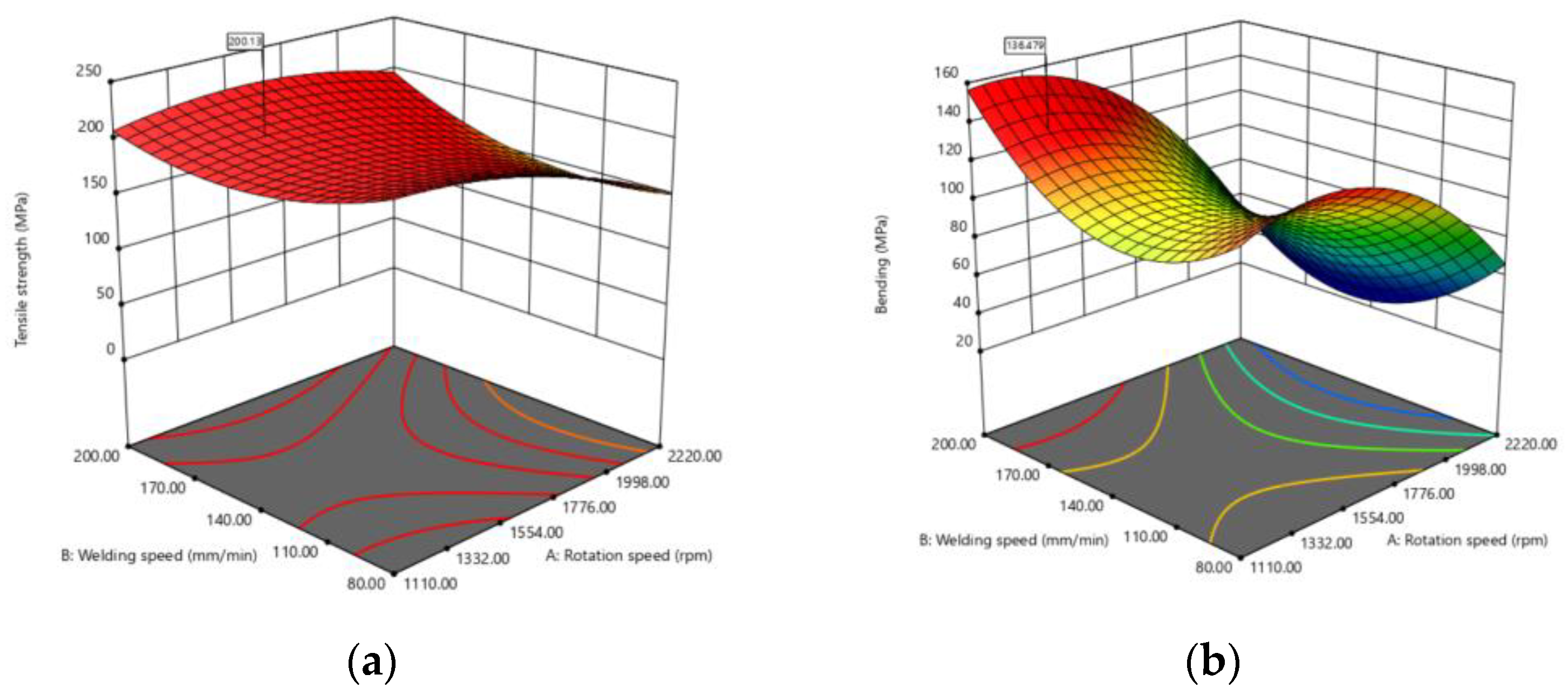
4.1. Optimization Process by D-Optimal Experimental Design

We designed the experiment using Design-Expert software. Five controlled parameters were set: rotational speed (S), welding speed (F), tool tilt angle (T), tool pin profile, and type. We used different rotation details for the specimens, as listed in

Table 6. Details of the tested specimens.

Material	Size (mm)	Thickness (mm)	Ultimate Tensile Strength (MPa)	Maximum Bending Strength (MPa)
(SSM) ADC12	75 × 150	6	208.53	153

.

The D-optimal experimental design produced 29 experiments, as shown in

Table 7. Actual design of experiments.

Run	Rotation Speed	Welding Speed	Tool Tilt Angle (Deg)	Tool Pin Profile	Rotational Direction	UTS (MPa)	MBS (MPa)
1	2062.92	142.75	3.41	Hexagon	ccw	96.28	83.56
2	1110.00	80.00	6.00	Hexagon	ccw	140.38	104.67
3	2023.17	168.30	4.03	Cylindrical	ccw	99.03	71.72
4	1803.75	200.00	6.00	Cylindrical	cw	91.02	110.31
5	1110.00	80.00	0.00	Cylindrical	ccw	43.65	42.01
6	2220.00	80.00	6.00	Cylindrical	cw	151.23	120.53
7	1110.00	80.00	6.00	Hexagon	ccw	134.11	117.65
8	1371.09	151.66	2.51	Cylindrical	ccw	53.49	45.42
9	1110.00	200.00	6.00	Hexagon	cw	137.95	103.91
10	1654.93	148.96	3.67	Hexagon	cw	166.65	122.85
11	2216.02	95.19	1.34	Cylindrical	ccw	44.85	56.84
12	1110.00	200.00	6.00	Hexagon	cw	131.38	100.34
13	1484.65	96.41	2.72	Hexagon	cw	159.49	122.32
14	2220.00	80.00	6.00	Cylindrical	cw	153.76	126.35
15	1705.76	134.87	2.91	Hexagon	cw	150.98	125.87
16	1715.48	141.78	3.18	Hexagon	ccw	126.76	113.28
17	1827.64	128.46	1.71	Cylindrical	cw	171.87	130.67
18	1110.00	80.00	0.00	Cylindrical	ccw	40.52	36.41
19	1395.44	112.16	3.28	Hexagon	cw	143.6	100.35
20	1307.14	164.53	2.04	Cylindrical	cw	155.18	117.82
21	1338.46	200.00	1.61	Cylindrical	ccw	49.51	35.91
22	1896.10	168.39	3.46	Hexagon	cw	162.96	125.98
23	1688.31	152.64	4.57	Hexagon	ccw	111.02	105.72
24	1893.30	167.26	1.61	Cylindrical	cw	130.02	112.65
25	1445.26	142.86	3.42	Cylindrical	ccw	51.59	54.29
26	1863.64	147.26	3.56	Hexagon	ccw	101.48	95.89
27	1391.97	143.76	4.03	Cylindrical	cw	121.32	88.65
28	1717.21	140.79	1.22	Cylindrical	cw	168.45	122.21
29	2062.92	142.75	3.41	Hexagon	ccw	97.46	65.27

; thus, 29 specimens were prepared, as shown in Figure 1.

After the welding process was finished, the ultimate tensile strength (UTS) and maximum bending strength (MBS) were measured using a tensile test machine (model NRI-TS501-300, Narin Instruments Co. Ltd., Bangmueng Mueng, Samutprakarn, Thailand; Figure 2). The welded specimens were tested until broken, and then the UTS and MBS were recorded, as shown in Table 7.

Table 7 provides the experimental results; the UTS and MBT of the workpiece were obtained from experiment number 17, which used a rotational speed of 1827.64 rpm, a welding speed of 128.46 mm/min, a tool tilt angle of 1.71°, a cylindrical pin profile, and clockwise rotation. This welding parameter produced the highest tensile strength of 171.87 MPa and highest bending strength of 130.67 MPa.

Based on the experimental results in Table 7, the D-optimal experimental design software produced a regression equation showing the relationship between the variable values. The ANOVA results for the UTS showed that the model forms were acceptable as mathematical models because the p-values of the quadratic model were lower than 0.05, and the model was statistically significant with a 95% confidence interval. The mathematical model had a coefficient of determination (R²) from the influence of variables equal to 95.26%, and the revised coefficient (adjusted R²) was greater than 86.73%, which confirmed that the regression model obtained the right format for the above UTS response, as shown in

Table 8. The ANOVA results for the tensile strength response using the Design-Expert software.

Source of Variation	Sum of Squares	DF	Mean Squares	F-Value	p-Value
Model	48,619.12	18	2701.06	11.17	0.0002
Linear	13,684.2	5	2736.83	11.31	0.001
Square	174.9	3	58.31	0.24	0.866
Interaction	8516.4	10	851.64	3.52	0.030
Residual Error	2418.8	10	241.88
Lack-of-Fit	2368.79	5	473.76	47.34	0.0003
Pure Error	50.0	5	10.01
Total	51,037.9	28
R-sq = 95.26%, R-sq (adj) = 86.73%

. Four models for the UTS were formulated as follows:

$$\begin{array}{ll}CW\_{ }_{Cylindrical}& =318+0.081 S-2.46 F-9.6T-0.000055 S\ast S+0.0065 F\ast F+1.56 t\ast t\\ & +0.000464 S\ast F+0.0060 S\ast T-0.162 F\ast T\end{array}$$

(21)

$$\begin{array}{ll}CC{W}_{\_} Cylindrical& =78+0.130 S-2.43 F+18.9 T-0.000055 S\ast S+0.0065 F\ast F+1.56 T\ast T\\ & +0.000464 S\ast F+0.0060 S\ast T-0.162 F\ast T\end{array}$$

(22)

$$\begin{array}{ll}CW\_ Hexagon& =306+0.030 S-1.33 F-22.7 T-0.000055 S\ast S+0.0065 F\ast F+1.56 T\ast T\\ & +0.000464 S\ast F+0.0060 S\ast T-0.162 F\ast T\end{array}$$

(23)

$$\begin{array}{ll}CCW\_ Hexagon& =82+0.079 S-1.30 F+5.8 T-0.000055 S\ast S+0.0065 F\ast F+1.56 T\ast T\\ & +0.000464 S\ast F+0.0060 S\ast T-0.162 F\ast T\end{array}$$

(24)

The ANOVA results for the MBS are shown in

Table 9. The ANOVA results for bending strength response using the Design-Expert software.

Source of Variation	Sum of Squares	DF	Mean Squares	F-Value	p-Value
Model	27,238.3	18	1513.24	17.31	0.000
Linear	5753.3	5	1150.66	13.16	0.000
Square	291.0	3	96.98	1.11	0.390
Interaction	4293.9	10	429.39	4.91	0.010
Residual Error	874.1	10	87.41
Lack-of-Fit	583.8	5	116.77	47.34	0.0003
Pure Error	290.3	5	58.06
Total	28,112.4	28
R-sq = 96.89%, R-sq (adj) = 91.29%

DF: degrees of freedom.

. The mathematical model had a coefficient of determination (R²) of 95.26% and the revised coefficient (adjusted R²) from the influence of variables was equal to 86.73%. The developed mathematical model for the MBS includes four models as follows:

$$\begin{array}{ll}CW\_{ }_{Cylindrical}& =-34+0.385 S-2.19 F-14.9 T-0.000106 S\ast S+0.01026 F\ast F-1.44 T\ast T\\ & -0.000350 S\ast F+0.01149 S\ast T-0.0288 F\ast T\end{array}$$

(25)

$$\begin{array}{ll}CC{W}_{\_} Cylindrical& =430+0.322 S-1.49 F-29.8 T-0.000106 S\ast S+0.01026 F\ast F-1.44 T\ast T\\ & -0.000350 S\ast F+0.01149 S\ast T-0.0288 F\ast T\end{array}$$

(26)

$$\begin{array}{ll}CW\_ Hexagon& =-59+0.383 S-2.88 F+11.7 T-0.000106 S\ast S+0.01026 F\ast F-1.44 T\ast T\\ & -0.000350 S\ast F+0.01149 S\ast T-0.0288 F\ast T\end{array}$$

(27)

$$\begin{array}{ll}CCW\_ Hexagon& =33+0.320 S-2.18 F-3.2 T-0.000106 S\ast S+0.01026 F\ast F-1.44 T\ast T\\ & -0.000350 S\ast F+0.01149 S\ast T-0.0288 F\ast T\end{array}$$

(28)

where S, F, and T represent the rotational speed, welding speed, and tool tilt angle, respectively. The D-optimal experimental design software was used to determine the optimal solution using the regression model in Equations (21)–(28). The parameters generating this solution were as follows: rotational speed of 1374.07 rpm, welding speed of 167.68 mm/min, tool tilt angle of 0.10°, cylindrical pin profile, and clockwise rotation. Responses were ultimate tensile strength (UTS) of 200.13 MPa, as shown in Figure 3a, and maximum bending strength (MBS) of 136.47 MPa, as shown in Figure 3b. The parameters generating this solution were as follows: rotational speed of 1893.30 rpm, welding speed of 167.26 mm/min, tool tilt angle of 1.610°, cylindrical pin profile, and clockwise rotation. Resulting multi-responses were UTS of 183.59 MPa and MBS of 141.71 MPa. The parameters generating this solution were as follows: rotational speed of 1995.75 rpm, welding speed of 90.72 mm/min, tool tilt angle of 4.94°, cylindrical pin profile, and counterclockwise rotation.

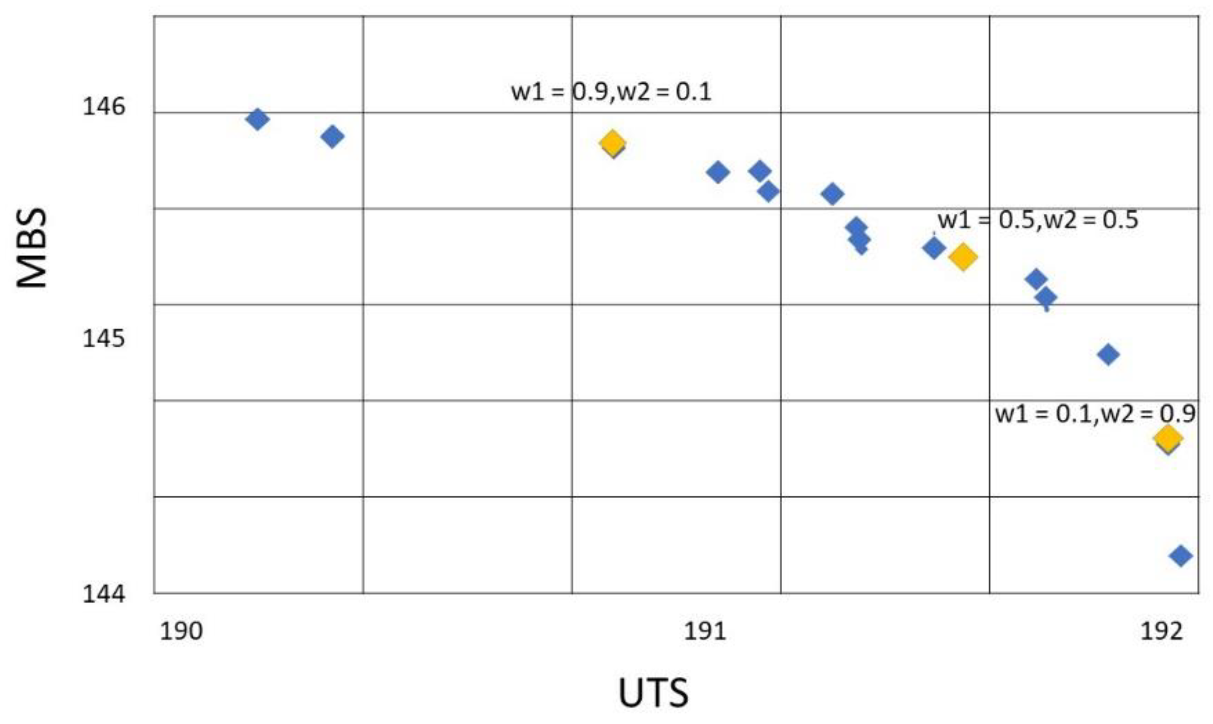
4.2. Results Using Multi-Objective Variable Neighborhood Strategy Adaptive Search (MOVaNSAS)

The proposed VaNSAS was coded in PyCharm (JetBrains Americas, Inc., Marlton, NJ, USA) using a PC with an Intel Core i7 3.70 GHz CPU and 8 GB DDR4 RAM. The objective function of the model was given by the D-optimal experimental design (Equations (21)–(24)) and we used VaNSAS to find the optimal solution to the problem subject of Equations (25)–(28). The ranges of the parameter values that can be applied using the D-optimal experimental design are shown in

Table 10. Pareto ratio of the proposed methods.

#No	#Iteration	MOGA		MODE		MOVaNSAS
(1)	(2)	#Pareto (3)	Ratio (3)/(2)	#Pareto (4)	Ratio (4)/(2)	#Pareto (5)	Ratio (5)/(2)
1	200	184	0.92	412	2.06	818	4.09
2	200	238	1.19	813	4.065	411	2.055
3	200	383	1.915	638	3.19	549	2.745
4	200	153	0.765	777	3.885	491	2.455
5	200	141	0.705	680	3.4	961	4.805
6	400	128	0.32	487	1.2175	991	2.4475
7	400	109	0.2725	473	1.1825	717	1.7925
8	400	88	0.22	586	1.465	869	2.1725
9	400	97	0.2425	507	1.2675	648	1.62
10	400	146	0.365	790	1.975	530	1.325
11	600	266	0.4433	677	1.1283	442	0.7366
12	600	138	0.23	500	0.8333	404	0.673
13	600	103	0.1716	803	1.3383	753	1.255
14	600	233	0.3883	463	0.7716	883	1.471
15	600	250	0.4166	789	1.315	527	0.8783
16	800	158	0.1975	496	0.62	896	1.12
17	800	100	0.125	414	0.5175	629	0.7862
18	800	260	0.325	553	0.6912	657	0.8212
19	800	509	0.6362	644	0.805	777	0.9712
20	800	141	0.1752	635	0.79375	920	1.15
21	1000	181	0.181	843	0.843	418	0.418
22	1000	226	0.226	583	0.583	491	0.491
23	1000	169	0.169	811	0.811	803	0.803
24	1000	162	0.162	738	0.738	662	0.662
25	1000	206	0.206	700	0.7	450	0.45
26	1200	88	0.073	685	0.5708	931	0.7758
27	1200	186	0.155	683	0.5691	672	0.56
28	1200	139	0.1158	754	0.6283	892	0.743
29	1200	391	0.3258	417	0.3475	975	0.8125
30	1200	154	0.1283	490	0.4083	878	0.7316
Average ratio			0.392		1.29		1.39

. The range of the ultimate tensile strength is not limited because it is the response of the input parameters that we aim to determine.

$$1100 \mathrm{rpm}\le S \le 2200 \mathrm{rpm},$$

(29)

$$80\frac{\mathrm{mm}}{\min }\le F \le 200\frac{\mathrm{mm}}{\min },$$

(30)

$$0 \mathrm{degrees}\le T \le 6 \mathrm{degrees}$$

(31)

In our experiment, the computational time was set to be the termination condition. It was set to 10 min for all proposed MOVaNSAS and compared methods (GA and DE). The Pareto fronts of all heuristics are shown in Figure 4 (MOGA), Figure 5 (MODE), and Figure 6 (MOVaNSAS).

Table 10 shows the compared performances of MODE, MOGA, and MOVaNSAS in finding the Pareto front. We tested the proposed methods by constructing the solution using a different number of iterations. All proposed methods used the same number of iterations and population, and the points in the Pareto front are counted and the ratio is calculated as $Ratio=\frac{Number of Points in Pareto Front}{Number of iteration}.$ The computational result is shown in Table 10. From the computational result, we found that MOVaNSAS gave the highest ratio, which means when we used equal iteration, MOVaNSAS gave the highest number of points in the Pareto front. The Pareto front in Table 10 was applied with TOPSIS to find the promising solution.

TOPSIS was applied to find the promising parameters using w1 and w2 = 0.5 (expertise suggestion). The results of TOPSIS for all methods are shown in

Table 11. The computational results of UTS and MBS of each heuristic.

Type of Rotational Direction/Tool Pin Profile	Output Values of Proposed Methods
	D-opt		MOGA		MODE		MOVaNSAS
	UTS	MBS	UTS	MBS	UTS	MBS	UTS	MBS
CW_Cylindrical	-	-	192.52	145.14	191.31	145.48	202.45	148.58
CW_Hexagon	-	-	172.71	144.96	177.31	142.16	201.65	147.25
CCW_Cylindrical	183.59	141.71	186.52	141.14	174.96	141.66	192.33	131.52
CCW_Hexagon	-	-	175.18	142.01	176.13	143.83	191.44	143.85

, and the level of parameters obtained from the promising solution is shown in

Table 12. The prediction result of optimal welding condition of each heuristic. The computational results of the ultimate tensile strength of each heuristic.

Method	Optimal Parameter					UTS	MBS
	Rotational Speed	Welding Speed	Tool Tilt	Pin Profile	Rotational Direction
D-optimal	1995.75	90.72	4.94	cylindrical	Counter clockwise	183.59	141.71
MODE	1534.11	84.28	0.502	cylindrical	clockwise	191.31	145.48
MOGA	1545.20	84.77	0.43	cylindrical	clockwise	192.52	145.14
MOVaNSAS	1469.44	80.35	1.01	cylindrical	clockwise	202.45	148.58

.

From the computational results shown in Table 11 and Table 12, the UTS and MBT of MOVaNSAS were 202.45 and 148.58 MPa, respectively. The UTS was better than MODE, MOGA, and D-opt by 5.58%, 5.15%, and 10.27%, respectively, and the MBS was better than MODE, MOGA, and D-opt by 2.23%, 2.13%, and 4.84%, respectively.

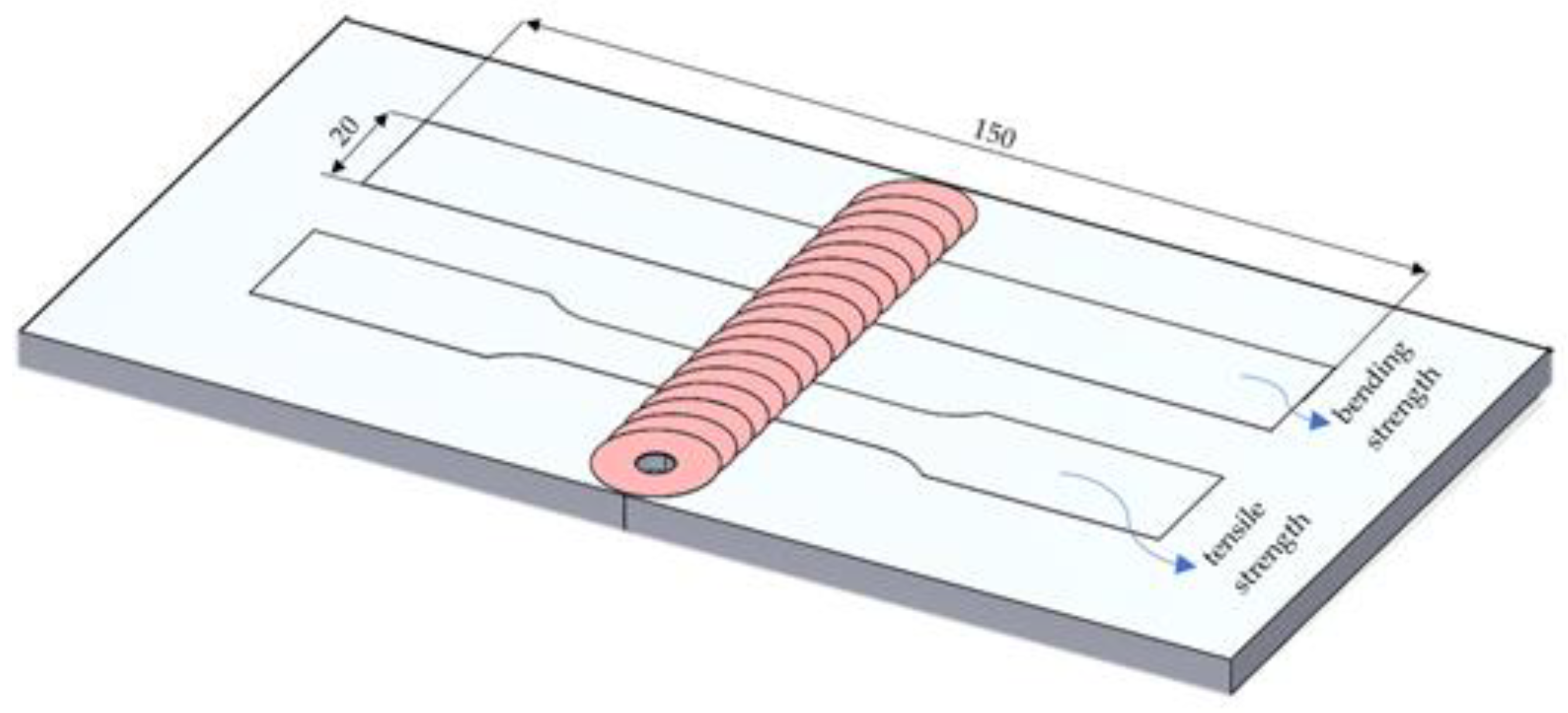
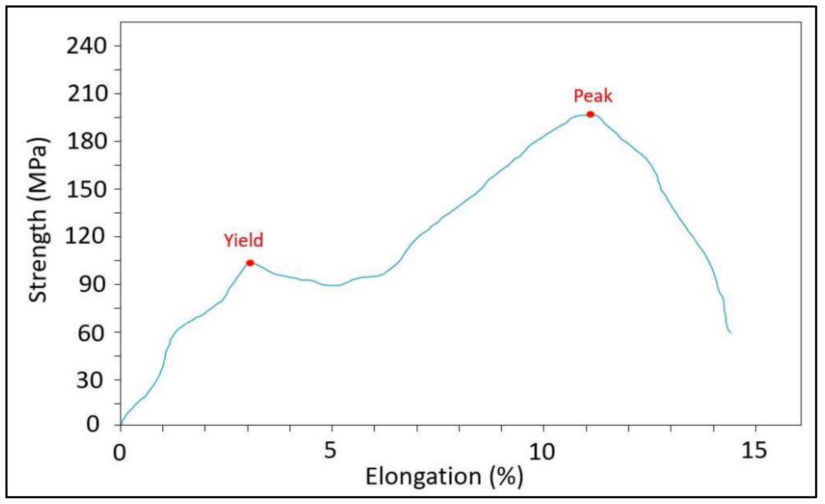
4.3. Verifying the Results by Testing Optimal Parameters with Actual Specimens

After we obtained the promising parameters from MOVaNSAS, as shown in Table 12, we performed a test and compared the results of confirmed experiments with the calculated MOVaNSAS results in order to check if the parameter values generated by VaNSAS could form a welded material with the UTS and MBS. Twelve replications were conducted, and the average ultimate tensile strength and average maximum bending strength were recorded, as shown in

Table 13. Comparison of the experimental and the MOVaNSAS results.

Variable Parameter	Unit	Result	UTS (MPa)			MBT (MPa)
			Confirmed Experiment	MOVaNSAS	% Difference	Confirmed Experiment	MOVaNSAS	% Difference
Rotational speed	rpm	1469.44	202.03 ± 0.251	202.45	0.208	148.10 ± 0.451	148.58	0.324
Welding speed	mm/min	80.35
Tool tilt	Deg	1.01
Pin profile	Cylindrical
Rotational direction	Clockwise

. In addition, the high performance of the weld line could be observed from the relationship between tensile strength and ductile property. The ductile property is considered from the elongation percentage by tensile testing. The elongation percentage or ductile value of the weld line shows a maximum elongation of 14.4% before damaging the weld line, as shown in Figure 7.

The difference in verifying the result and prediction value can be calculated by Equation (32):

$$\%diff= \frac{UTS/MBT{ }^{Exp}-UTS/MBT{ }^{\mathrm{MOVaNSAS}}}{UTS/MB{T}^{Exp}}\times 100\%$$

(32)

where $UTS/MBT{ }^{Exp}$ is the UTS or MBT generated by the experiment and UTS/MBT^MOVaNSAS is the UTS or MBT generated by MOVaNSAS. The average UTS and MBT obtained from our experiment were 0.208% and 0.324% better, respectively, than the original values. Next, we explain the microstructure of the material from the experiment specimens.

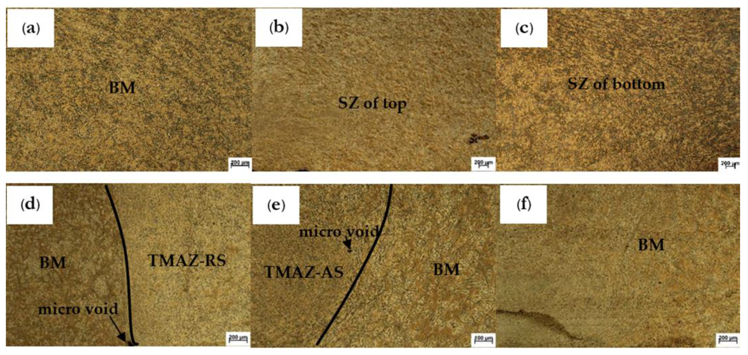
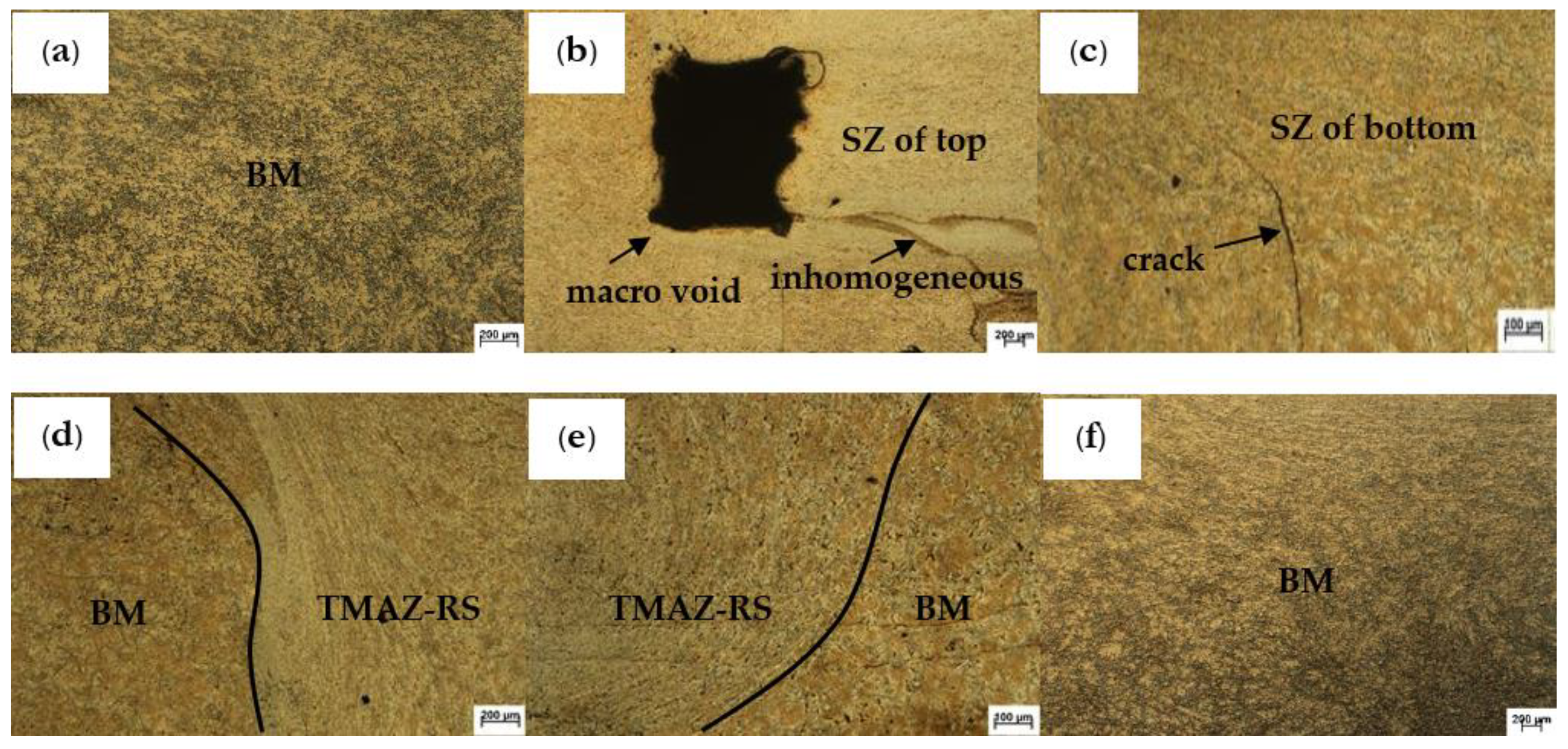
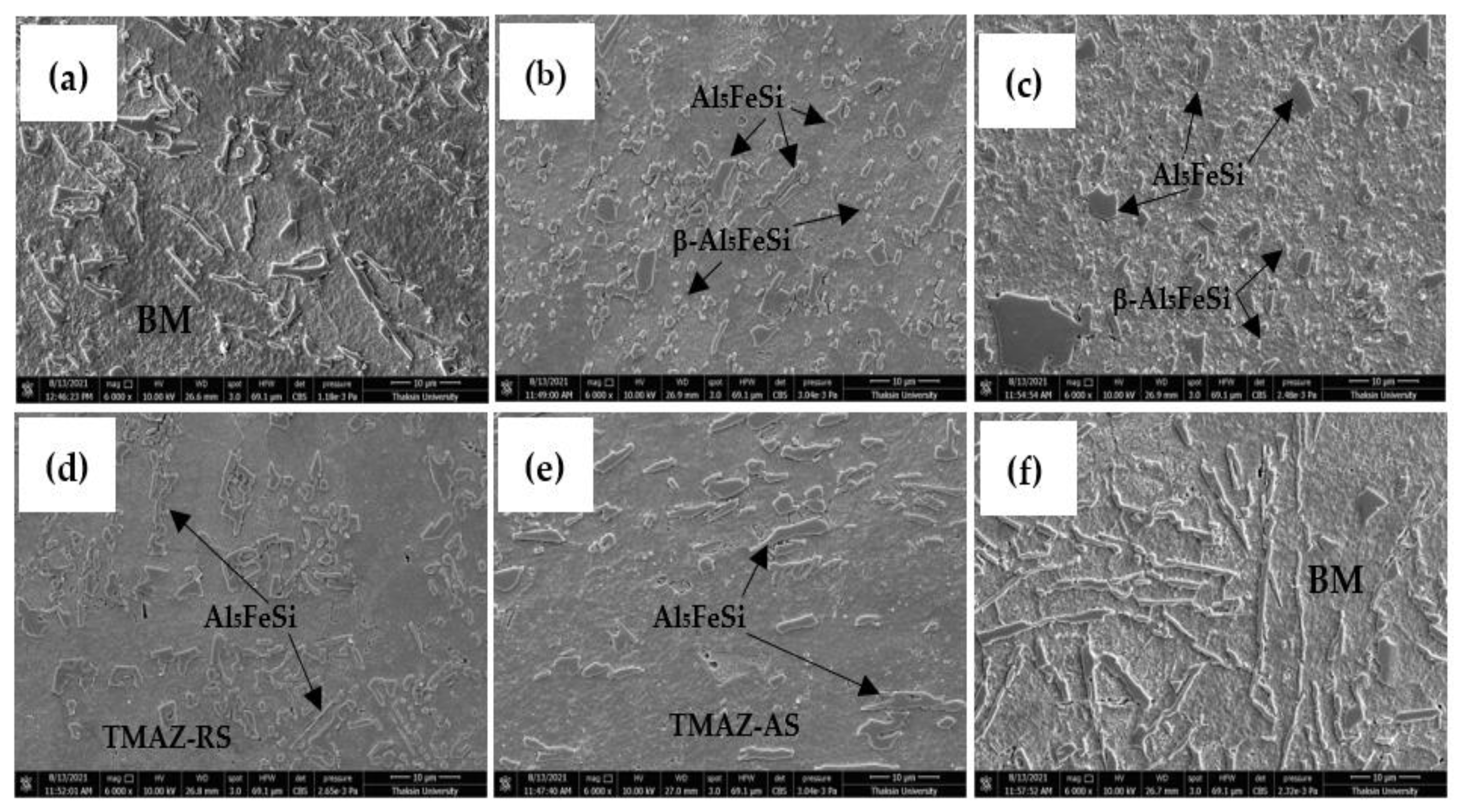
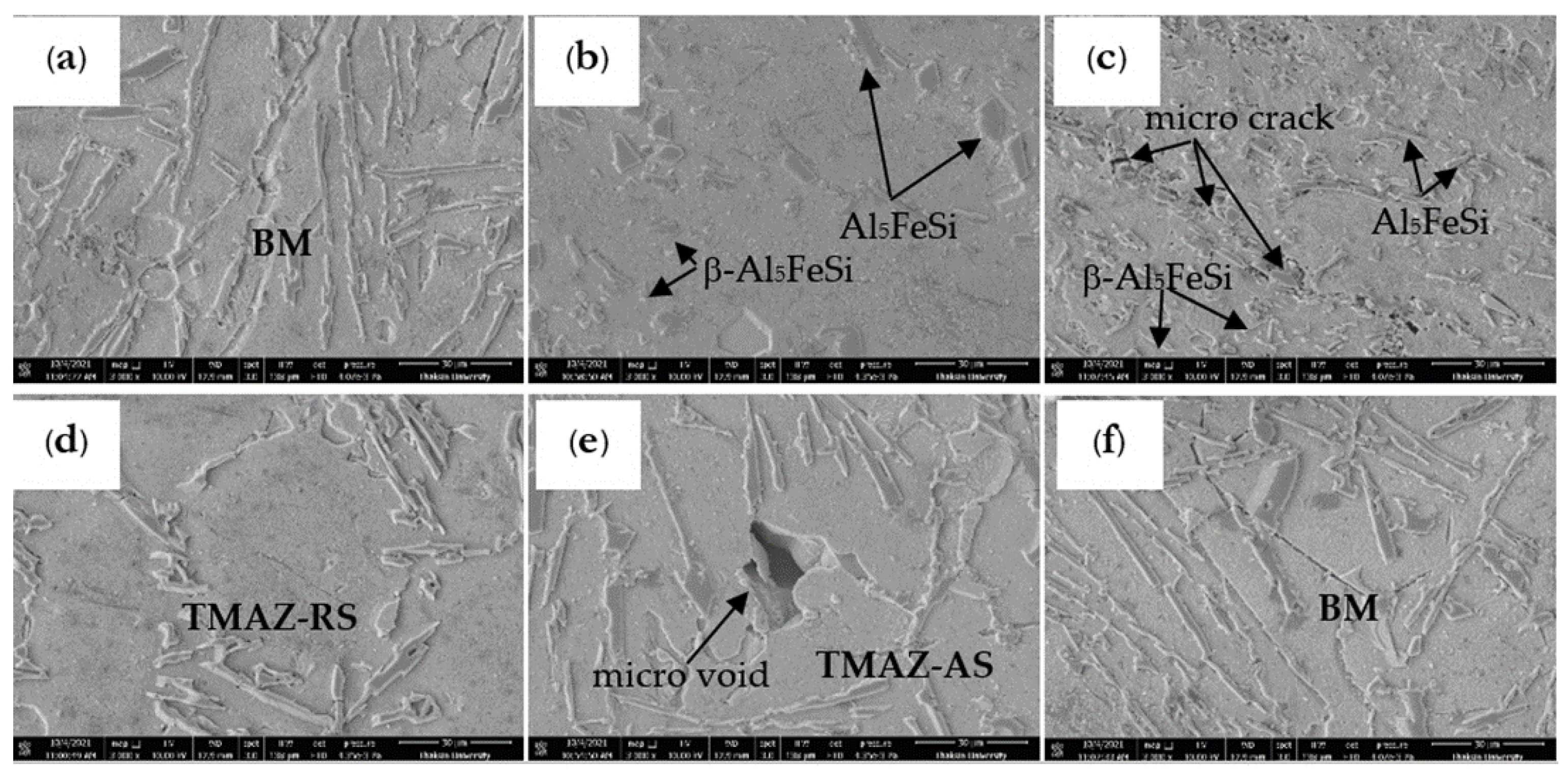
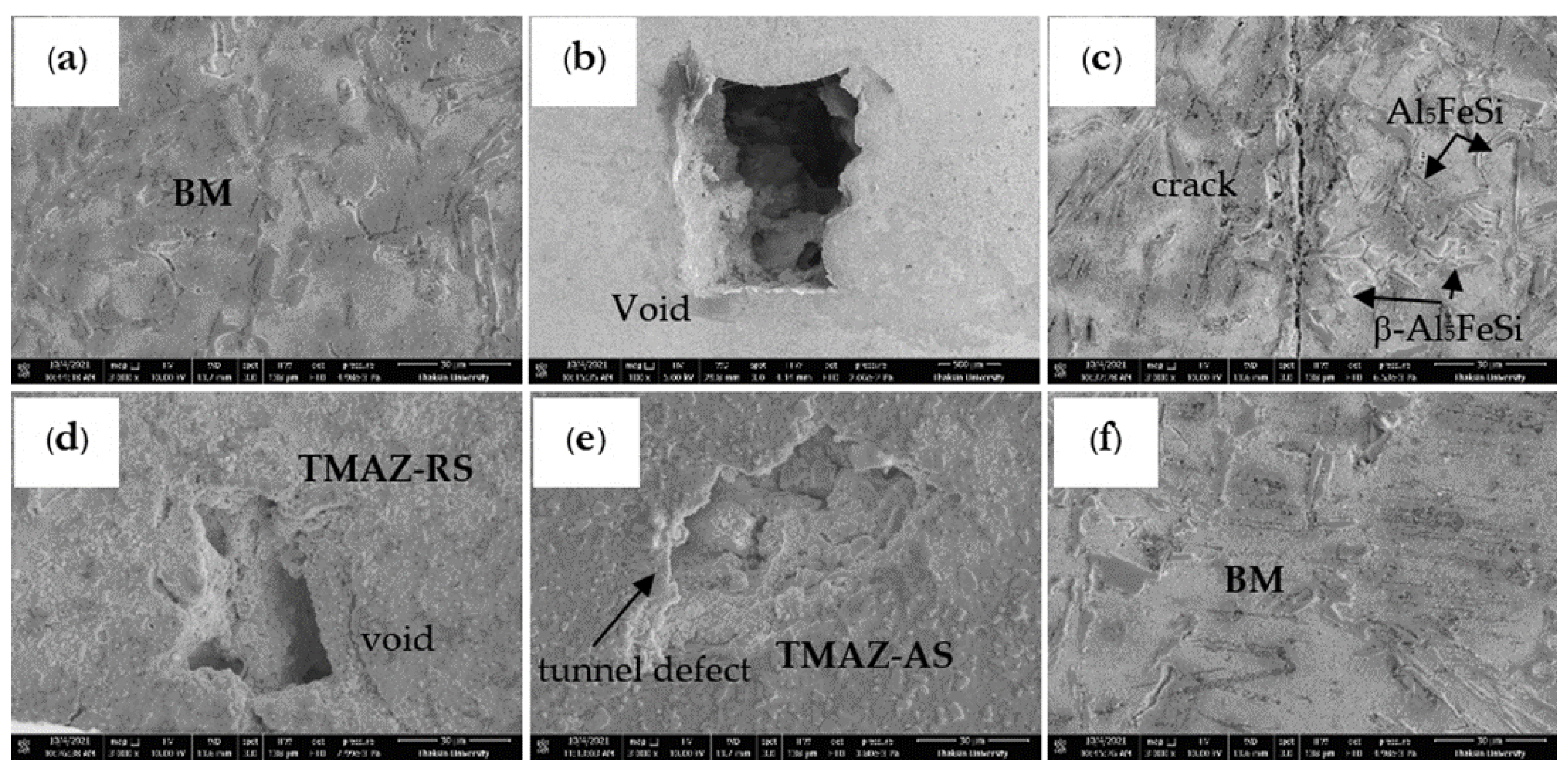
4.4. Microstructure Analysis

The defect formation and microstructure were analyzed by three approaches: optical microscope (OM), scanning electron microscope (SEM), and EDX-ray spectroscopy. For the welding, the optimized parameter conditions were rotation speed of 1469.44 rpm, welding speed of 80.35 mm/min, tilt angle of 1.01°, cylindrical tool, and clockwise direction, which resulted in no groove defects or discontinuity. The full weld seam of the welding parameters from MOVaNSAS shows the weld line without defects, as shown in Figure 8a, due to the optimal welding conditions of MOVaNSAS, including suitable relational parameters during tool rotation speed and welding speed at a ratio of 18.62. This relational ratio is not over a ratio of 50 and not over a heat level in FSW, showing smooth-surface weld joints without groove defects on the surface [8,74,75,76,77].

The microstructural result of the optimized welding parameters exhibited a changing structural deformation in the weld joint area that was transferred from the FSW process of SSM-ADC12 aluminum material. After FSW, the grain of the weld seam showed changes in the grain size from the base material to the welding zone, as shown in Figure 8b. The grain size in the welding zone is on average 10 µm, decreasing from the base material by 75%.

The weld line structure displayed a difference in deformation in the retreating side (RS) and advancing side (AS), as shown in Figure 9. The thermomechanical affected zone (TMAZ) affected tool stirring and heat in the process. The observed characteristics of the microstructure in the TMAZ-RS and TMAZ-AS were material deformations from the mechanical force of tool stirring and the heat expanding effect in welding. The tool stirring and heat effect in the welding process incurred material flow in the rotational direction and structural deformation. Therefore, the TMAZ-RS and TMAZ-AS areas exhibited differences in the microstructure of the base material that are shown in Figure 9d,e. Whereas the stir zone (SZ) showed a sound weld joint, the interweave material flow and homogeneous material mixing led to recrystallization and structural completeness without defects in the weld joint. The SZ structures of both the top and bottom zones are shown in Figure 9b,c. The base material (BM) area exhibited slight changes in grain growth because of the heat of the welding processes that generated high heat during joint welding, and the heat extended from the TMAZ to the BM area. Therefore, some microstructures in the BM changed in the intimate zone of the TMAZ without difficulty. Characteristics of nearby structures of the original material are displayed in Figure 9a,f.

The weld line of the optimized conditions from D-optimal showed a microdefect in the TMAZ (Figure 10d,e). The SZ displayed a fine grain, but inhomogeneous material in Figure 10b,c. The greater degree of the tool tilt angle caused the material to flow and mix in the weld seam. In addition, the TMAZ of both RS and AS exhibited material deformation and extended grain following the rotational direction that effectively increased the dislocation of equiaxed grains. Although increased dislocation density increased the weld line strength, the microvoid defect appearing in the structure was a problem of reduced tensile and bending strength. Therefore, the weld seam from the D-optimal prediction gave lower tensile and bending strength than the MOVaNSAS prediction. The microstructure of the best initial experiment showed a large void and a crack defect in the SZ (Figure 11b,c). The structure in the weld line is not homogenous and has a less fine grain than both structures of the D-optimal approach and the MOVaNSAS approach in the SZ. Moreover, the material deformation from stirring appears as large equiaxed grains in the TMAZ (see Figure 11d,e), which have a low density of grain dislocation. Therefore, this welding condition gave lower tensile and bending strength than the optimal condition of the D-optimal approach and MOVaNSAS.

The consideration of phase in structure was evaluated by SEM for each optimal welding parameter. The weld joint structure of the MOVaNSAS approach displayed an Al₅FeSi intermetallic compound phase in the SZ that appears to be split into large particle sizes and uniform distribution. The Al₅FeSi intermetallic compounds were separated by tool stirring and by bumping into the tool tilt angle. Regarding rotation speed and welding speed, a suitable ratio was useful in the material flow and uniform distribution of intermetallic particles. The particle size of the Al₅FeSi phase was smaller than 10 µm and had a spiky appearance that is shown in Figure 12b,c. The β-Al₅FeSi phase had smaller fine particles than the Al₅FeSi phase and uniform dispersion that produced a density of dislocation. Therefore, the density of the Al₅FeSi and β-Al₅FeSi phases could improve the mechanical properties of tensile and bending strength. In the same way, the TMAZ indicated that the Al₅FeSi phase had a long shape that was small, as well. The Al₅FeSi phase in the TMAZ showed a larger size than the Al₅FeSi phase in the SZ because of low heat energy and deformation of low material in the TMAZ (Figure 12d,e). Thus, the TMAZ areas were appearing as a weaker mechanical property than SZ. Moreover, the BM of the SSM-ADC12 aluminum alloy showed the largest Al₅FeSi phase, which was larger than the other zones in the structural weld joint, as seen in Figure 12a,f. The arrangement of the Al₅FeSi phase had a smooth and even distribution. The Al₅FeSi phase was rod-shaped and arranged along the grain boundary of the material.

The weld joint structure of the D-optimal approach exhibited lower β-Al₅FeSi intermetallic phase dispersion than the structure of the MOVaNSAS approach in the SZ. The Al₅FeSi intermetallic compounds exhibited large particles and low distribution when compared with the MOVaNSAS approach, as shown in Figure 13b,c. Moreover, the SZ area displayed microcracking and microvoids in the TMAZ of AS, which led to weakness in the weld line. The microstructure of the best initial experiment displayed the largest void defect and cracking in the SZ and TMAZ, as shown in Figure 14. In addition, the β-Al₅FeSi intermetallic phase was not uniformly dispersed, as observed in Figure 14b,c.

The concentration of the alloying elements in the SZ was evaluated by EDX-ray spectroscopy. The weld seam structure of the MOVaNSAS approach was checked for the elemental composition of the Al₅FeSi phase of new crystallization and intermetallic compound formation. The Al₅FeSi phase change in particle size and distribution of phase was influenced by the heat input and experimental parameters. The Al₅FeSi phase formed from the Mg₂Si phase because the Fe element separated the Mg₂Si phase formation, as shown in Figure 15.

The heat input during FSW was in the range of 330–520 °C. Thus, it was possible for the formation of the Al₈Fe₂Si and Al₄FeSi₂ phases, which had favorable solubility in solid solution at high temperature. It is worth noting that the O element occurred during welding, resulting in a new compound phase. The O element led to Al₂O₃ and SiO₂ phase formation, which were widely dispersed according to the analysis. The Al₂O₃ and SiO₂ phases were resistant to tensile and bending forces as well, but both phases were increasingly embedded in the material and reduced the prominence of mechanical properties such as elongation and ductile property. Therefore, a decrease in certain mechanical properties may lead to fracture of the weld seams.

5. Conclusions

With this research, we aimed at finding the optimal welding parameters to maximize the ultimate tensile and bending strength in FSW of SSM-ADC12. The optimal welding conditions for prediction with the MOVaNSAS algorithm were a rotation speed of 1469.44 rpm, welding speed of 80.35 mm/min, tilt angle of 1.01°, a cylindrical pin tool, and a clockwise rotational direction. This condition gave the highest UTS of 202.45 MPa, and MBS of 148.58 MPa. The optimal welding conditions were tested for accuracy and reliability by performing the experiment, and the result showed differences of 0.203% and 0.287% for UTS and MBS, respectively. MOVaNSAS predicted UTS better than MODE, MOGA, and D-opt by 5.58%, 5.15%, and 10.27%, respectively, while it predicted MBS better than MODE, MOGA, and D-opt by 2.23%, 2.13%, and 4.84%, respectively. From this result, we can confirm that MOVaNSAS is an effective algorithm to predict the optimal parameters of the target material. The weld line structure in the optimal welding parameters showed no defect or precipitation of the small intermetallic phases Al₅FeSi and β-Al₅FeSi with uniform distribution. The intermetallic phase uniform dispersion led to a phenomenon of a dislocation strength mechanism, which increased both the tensile and bending mechanical properties.

However, use of the weld joint will require several properties from usable milieu. Therefore, a weld seam should have several supplementary properties in the weld joint, especially impact resistance, which is one of the most important mechanical properties of the weld line.

References

1. Guo, H.; Hu, J.; Tsai, H.L. Formation of weld crater in GMAW of aluminum alloys. Int. J. Heat Mass Transf. 2009, 52, 5533–5546. [Google Scholar] [CrossRef]
2. Da Silva, C.L.M.; Scotti, A. The influence of double pulse on porosity formation in aluminum GMAW. J. Mater. Process. Technol. 2006, 171, 366–372. [Google Scholar] [CrossRef]
3. Fang, X.; Zhang, J. Effect of underfill defects on distortion and tensile properties of Ti-2Al-1.5Mn welded joint by pulsed laser beam welding. Int. J. Adv. Manuf. Technol. 2014, 74, 699–705. [Google Scholar] [CrossRef]
4. Bhujangrao, T.; Froustey, C.; Iriondo, E.; Veiga, F.; Darnis, P.; Mata, F.G. Review of Intermediate Strain Rate Testing Devices. Metals 2020, 10, 894. [Google Scholar] [CrossRef]
5. Thomas, W.M.; Johnson, K.I.; Wiesner, C.S. Friction stir welding—Recent developments in tool and process technologies. Adv. Eng. Mater. 2003, 5, 485–490. [Google Scholar] [CrossRef]
6. Thomas, W.M.; Nicholas, E.D. Friction stir welding for the transportation industries. Mater. Des. 1997, 18, 269–273. [Google Scholar] [CrossRef]
7. Threadgill, P.L.; Leonard, A.J.; Shercliff, H.R.; Withers, P.J. Friction stir welding of aluminium alloys. Pap. Presented Int. Mater. Rev. 2009, 54, 49–93. [Google Scholar] [CrossRef]
8. Lakshminarayanan, A.; Malarvizhi, S.; Balasubramanian, V. Developing friction stir welding window for AA2219 aluminium alloy. Trans. Nonferrous Met. Soc. China 2011, 21, 2339–2347. [Google Scholar] [CrossRef]
9. Guo, J.F.; Chen, H.C.; Sun, C.N.; Bi, G.; Sun, Z.; Wei, J. Friction stir welding of dissimilar materials between AA6061 and AA7075 Al alloys effects of process parameters. Mater. Des. 2014, 56, 185–192. [Google Scholar] [CrossRef]
10. Hoyos, E.; Escobar, S.; Backer, J.D.; Martin, J.; Palacio, M. Manufacturing Concept and Prototype for Train Component Using the FSW Process. J. Manuf. Mater. Process. 2021, 5, 19. [Google Scholar] [CrossRef]
11. Giraud, L.; Robe, H.; Claudin, C.; Desrayaud, C.; Bocher, P.; Feulvarch, E. Investigation into the dissimilar friction stir welding of AA7020-T651 and AA6060-T6. J. Mater. Process. Technol. 2016, 235, 220–230. [Google Scholar] [CrossRef]
12. Bisadi, H.; Tavakoli, A.; Sangsaraki, M.T.; Sangsaraki, K.T. The influences of rotational and welding speeds on microstructures and mechanical properties of friction stir weld Al5083 and commercially pure copper sheets lap joint. Mater. Des. 2013, 43, 80–88. [Google Scholar] [CrossRef]
13. Kadaganchi, R.; Gankidi, M.R.; Gokhale, H. Optimization of process parameters of aluminum alloy AA 2014-T6 friction stir welds by response surface methodology. Def. Technol. 2015, 11, 209–219. [Google Scholar] [CrossRef] [Green Version]
14. Khan, N.Z.; Khan, Z.A.; Siddiquee, A.N. Effect of shoulder diameter to pin diameter (D/d) ratio on tensile strength of friction stir welded 6063 aluminium alloy. Mater. Today: Proc. 2015, 2, 1450–1457. [Google Scholar] [CrossRef]
15. Liu, H.; Zhang, H.; Pan, Q.; Yu, L. Effect of friction stir welding parameters on microstructural characteristics and mechanical properties of 2219-T6 aluminum alloy joints. Int. J. Mater. Form. 2012, 5, 235–241. [Google Scholar] [CrossRef]
16. Elangovan, K.; Balasubramanian, V. Influences of tool pin profile and welding speed on the formation of friction stir processing zone in AA2219 aluminium alloy. J. Mater. Process. Technol. 2008, 200, 163–175. [Google Scholar] [CrossRef]
17. Maeda, M.; Liu, H.; Fujii, H.; Shibayanagi, T. Temperature field in the vicinity of fsw-tool during friction stir welding of aluminium alloys. Weld. World 2005, 49, 69–75. [Google Scholar] [CrossRef]
18. Ilangovan, M.; Boopathy, S.R.; Balasubramanian, V. Effect of tool pin profile on microstructure and tensile properties of friction stir welded dissimilar AA 6061eAA 5086 aluminium alloy joints. Def. Technol. 2015, 11, 174–184. [Google Scholar] [CrossRef] [Green Version]
19. RajKumar, V.; VenkateshKannan, M.; Sadeesh, P.; Arivazhagan, N.; Ramkumar, K.D. Studies on Effect of Tool Design and Welding Parameters on the Friction Stir Welding of Dissimilar Aluminium Alloys AA 5052–AA 6061. Procedia Eng. 2014, 75, 93–97. [Google Scholar] [CrossRef] [Green Version]
20. Meengam, C.; Sillapasa, K. Evaluation of Optimization Parameters of Semi-Solid Metal 6063 Aluminum Alloy from Friction Stir Welding Process Using Factorial Design Analysis. J. Manuf. Mater. Process. 2020, 4, 123. [Google Scholar] [CrossRef]
21. Koilraj, M.; Sundareswaran, V.; Vijayan, S.; Rao, S.R.K. Friction stir welding of dissimilar aluminum alloys AA2219 to AA5083 Optimization of process parameters using Taguchi technique. Mater. Des. 2012, 42, 1–7. [Google Scholar] [CrossRef]
22. Bayazid, S.M.; Farhangi, H.; Ghahramani, A. Investigation of Friction Stir Welding Parameters of 6063-7075 Aluminum Alloys by Taguchi Method. Procedia Mater. Sci. 2015, 11, 6–11. [Google Scholar] [CrossRef] [Green Version]
23. Palani, K.; Elanchezhian, C. Multi response Optimization of Friction stir welding process parameters in dissimilar alloys using Grey relational analysis. IOP Conf. Ser. Mater. Sci. Eng. 2018, 390, 1–9. [Google Scholar] [CrossRef]
24. Aydin, H.; Bayram, A.; Esme, U.; Kazancoglu, Y.; Guven, O. Application of Grey Relation Analysis (GRA) and Taguchi Method for the Parametric Optimization of Friction Stir Welding (FSW) Process. Mater. Technol. 2010, 44, 205–211. [Google Scholar]
25. Shanavas, S.; Dhas, J.E.R. Parametric optimization of friction stir welding parameters of marine grade aluminium alloy using response surface methodology. Trans. Nonferrous Met. Soc. China 2017, 27, 2334–2344. [Google Scholar] [CrossRef]
26. Srichok, T.; Pitakaso, R.; Sethanan, K.; Sirirak, W.; Kwangmuang, P. Combined Response Surface Method and Modified Differential Evolution for Parameter Optimization of Friction StirWelding. Processes 2020, 8, 1080. [Google Scholar] [CrossRef]
27. Teimouri, R.; Baseri, H. Forward and backward predictions of the friction stir welding parameters using fuzzy-artificial bee colony-imperialist competitive algorithm systems. J. Intell. Manuf. 2013, 26, 307–319. [Google Scholar] [CrossRef]
28. Shojaeefard, M.H.; Behnagh, R.A.; Akbari, M.; Givi, M.K.B.; Farhani, F. Modelling and Pareto optimization of mechanical properties of friction stir welded AA7075/AA5083 butt joints using neural network and particle swarm algorithm. Mater. Des. 2013, 44, 190–198. [Google Scholar] [CrossRef]
29. Wakchaure, K.N.; Thakur, A.G.; Gadakh, V.; Kumar, A. Multi-Objective Optimization of Friction Stir Welding of Aluminium Alloy 6082-T6 Using hybrid Taguchi-Grey Relation Analysis- ANN Method. Mater. Today: Proc. 2018, 5, 7150–7159. [Google Scholar] [CrossRef]
30. Hartl, R.; Praehofer, B.; Zaeh, M. Prediction of the surface quality of friction stir welds by the analysis of process data using Artificial Neural Networks. Proc. Inst. Mech. Eng. Part. L J. Mater. Des. Appl 2020, 234, 732–751. [Google Scholar] [CrossRef]
31. Cisko, A.R.; Jordon, J.B.; Amaro, R.L.; Allison, P.G.; Wlodarski, J.S.; McClelland, Z.B.; Garcia, L.; Rushing, T.W. A parametric investigation on friction stir welding of Al-Li 2099. Mater. Manuf. Process. 2020, 35, 1–8. [Google Scholar] [CrossRef]
32. Shaik, B.; Gowd, G.H.; Prasad, B.D. Investigations and optimization of friction stir welding process to improve microstructures of aluminum alloys. Cogent Eng. 2019, 6, 1–14. [Google Scholar] [CrossRef]
33. Aldalur, E.; Suárez, A.; Veiga, F. Metal transfer modes for Wire Arc Additive Manufacturing Al-Mg alloys: Influence of heat input in microstructure and porosity. J. Mater. Process. Technol. 2021, 297, 117271. [Google Scholar] [CrossRef]
34. Khodabakhshi, F.; Gerlich, A.P. On the correlation between indentation hardness and tensile strength in friction stir processed materials. Mater. Sci. Eng. A 2020, 789, 1–14. [Google Scholar] [CrossRef]
35. Chen, H.; Cai, L.-X. Theoretical Conversions of Different Hardness and Tensile Strength for Ductile Materials Based on Stress–Strain Curves. Metall. Mater. Trans. A 2018, 49, 1090–1101. [Google Scholar] [CrossRef]
36. Shojaeefard, M.H.; Akbari, M.; Asadi, P. Multi objective optimization of friction stir welding parameters using FEM and neural network. Int. J. Precis. Eng. Manuf. 2014, 15, 2351–2356. [Google Scholar] [CrossRef]
37. Senthil, S.M.; Parameshwaran, R.; Nathan, S.R.; Kumar, M.B.; Deepandurai, K. A multi-objective optimization of the friction stir welding process using RSM-based-desirability function approach for joining aluminum alloy 6063-T6 pipes. Struct. Multidiscip. Optim. 2020, 62, 1117–1133. [Google Scholar] [CrossRef]
38. Gupta, S.K.; Pandey, K.; Kumar, R. Multi-objective optimization of friction stir welding process parameters for joining of dissimilar AA5083/AA6063 aluminum alloys using hybrid approach. Proc. Inst. Mech. Eng. Part L J. Mater. Des. Appl. 2016, 232, 343–353. [Google Scholar] [CrossRef]
39. Sharma, N.; Khan, Z.A.; Siddiquee, A.N.; Wahid, M.A. Multi-response optimization of friction stir welding process parameters for dissimilar joining of Al6101 to pure copper using standard deviation based TOPSIS method. Proc. Inst. Mech. Eng. Part C J. Mech. Eng. Sci. 2019, 233, 6473–6482. [Google Scholar] [CrossRef]
40. Goyal, A.; Garg, R.K. Parametric optimization of friction stir welding process for marine grade aluminum alloy. Int. J. Struct. Integr. 2018, 10, 1–15. [Google Scholar] [CrossRef]
41. Babu, K.K.; Panneerselvam, K.; Sathiya, P.; Haq, A.N.; Sundarrajan, S.; Mastanaiah, P.; Murthy, C.V.S. Parameter optimization of friction stir welding of cryorolled AA2219 alloy using artificial neural network modeling with genetic algorithm. Int. J. Adv. Manuf. Technol. 2017, 94, 3117–3129. [Google Scholar] [CrossRef]
42. Tamjidy, M.; Baharudin, B.T.H.T.; Paslar, S.; Matori, K.A.; Sulaiman, S.; Fadaeifard, F. Multi-Objective Optimization of Friction Stir Welding Process Parameters of AA6061-T6 and AA7075-T6 Using a Biogeography Based Optimization Algorithm. Materials 2017, 10, 533. [Google Scholar] [CrossRef] [Green Version]
43. Kesharwani, R.K.; Panda, S.K.; Pal, S.K. Multi Objective Optimization of Friction Stir Welding Parameters for Joining of Two Dissimilar Thin Aluminum Sheets. Procedia Mater. Sci. 2014, 6, 178–187. [Google Scholar] [CrossRef] [Green Version]
44. Roshan, S.B.; Jooibari, M.B.; Teimouri, R.; Asgharzadeh-Ahmadi, G.; Falahati-Naghibi, M.; Sohrabpoor, H. Optimization of friction stir welding process of AA7075 aluminum alloy to achieve desirable mechanical properties using ANFIS models and simulated annealing algorithm. Int. J. Adv. Manuf. Technol. 2013, 69, 1803–1818. [Google Scholar] [CrossRef]
45. Jirasirilerd, G.; Pitakaso, R.; Sethanan, K.; Kaewman, S.; Sirirak, W.; Kosacka-Olejnik, M. Simple Assembly Line Balancing Problem Type 2 By Variable Neighborhood Strategy Adaptive Search: A Case Study Garment Industry. J. Open Innov. Technol. Mark. Complex. 2020, 6, 21. [Google Scholar] [CrossRef] [Green Version]
46. Theeraviriya, C.; Sirirak, W.; Praseeratasang, N. Location and Routing Planning Considering Electric Vehicles with Restricted Distance in Agriculture. World Electr. Veh. J. 2020, 11, 61. [Google Scholar] [CrossRef]
47. Theeraviriya, C.; Ruamboon, K.; Praseeratasang, N. Solving the multi-level location routing problem considering the environmental impact using a hybrid metaheuristic. Int. J. Eng. Bus. Manag. 2021, 13, 1–17. [Google Scholar] [CrossRef]
48. Kusoncum, C.; Sethanan, K.; Pitakaso, R.; Hartl, R.F. Heuristics with novel approaches for cyclical multiple parallel machine scheduling in sugarcane unloading systems. Int. J. Prod. Res. 2020, 59, 1–19. [Google Scholar] [CrossRef]
49. Khamsing, N.; Chindaprasert, K.; Pitakaso, R.; Sirirak, W.; Theeraviriya, C. Modified ALNS Algorithm for a Processing Application of Family Tourist Route Planning: A Case Study of Buriram in Thailand. Computation 2021, 9, 23. [Google Scholar] [CrossRef]
50. Pitakaso, R.; Sethanan, K.; Theeraviriya, C. Variable neighborhood strategy adaptive search for solving green 2-echelon location routing problem. Comput. Electron. Agric. 2020, 173, 1–12. [Google Scholar] [CrossRef]
51. Pitakaso, R.; Sethanan, K.; Jirasirilerd, G.; Golinska-Dawson, P. A novel variable neighborhood strategy adaptive search for SALBP-2 problem with a limit on the number of machine’s types. Ann. Oper. Res. 2021, 298, 1–25. [Google Scholar] [CrossRef]
52. Amir, H.L.; Salman, N. Effect of Welding Parameters on Microstructure, Thermal, and Mechanical Properties of Friction-Stir Welded Joints of AA7075-T6 Aluminum Alloy. Metall. Mater. Trans. A 2014, 45A, 2792–2807. [Google Scholar]
53. Ramesha, K.; Sudersanan, P.; Santhosh, N.; Sasidhar, J. Design and optimization of the process parameters for friction stir welding of dissimilar aluminium alloys. Eng. Appl. Sci. Res. 2021, 48, 257–267. [Google Scholar]
54. Tongne, A.; Desrayaud, C.; Jahazi, M.; Feulvarch, E. On material flow in Friction Stir Welded Al alloys. J. Mater. Process. Technol. 2017, 239, 284–296. [Google Scholar] [CrossRef]
55. Elyasi, M.; Derazkola, H.A.; Hosseinzadeh, M. Investigations of tool tilt angle on properties friction stir welding of A441 AISI to AA1100 aluminium. Proc. Inst. Mech. Eng. Part B J. Eng. Manuf. 2016, 230, 1–8. [Google Scholar] [CrossRef]
56. Meshram, S.D.; Reddy, G.M. Influence of Tool Tilt Angle on Material Flow and Defect Generation in Friction Stir Welding of AA2219. Def. Sci. J. 2018, 68, 512–518. [Google Scholar] [CrossRef]
57. Thimmaraju, P.K.; Arakanti, K.; Reddy, G.C.M. Influence of Tool Geometry on Material Flow Pattern in Friction Stir Welding Process. Int. J. Theor. Appl. Mech. 2017, 12, 445–458. [Google Scholar]
58. Zhang, Y.N.; Cao, X.; Larose, S.; Wanjara, P. Review of tools for friction stir welding and processing. Can. Metall. Q. 2012, 51, 250–261. [Google Scholar] [CrossRef]
59. Zhao, H.; Shen, Z.; Booth, M.; Wen, J.; Fu, L.; Gerlich, A. Calculation of welding tool pin width for friction stir welding of thin overlapping sheets. Int. J. Adv. Manuf. Technol. 2018, 98, 1721–1731. [Google Scholar] [CrossRef]
60. Grätzel, M.; Hasieber, M.; Löhn, T.; Bergmann, J. Reduction of friction stir welding setup loadability, process forces and weld seam width by tool scaling. Proc. IMechE Part L J. Mater. Des. Appl. 2020, 234, 1–10. [Google Scholar] [CrossRef]
61. Schmidt, H.; Hattel, J.; Wert, J. An analytical model for the heat generation in friction stir welding. Model. Simul. Mater. Sci. Eng. 2003, 12, 143–157. [Google Scholar] [CrossRef]
62. Malarvizhi, S.; Balasubramanian, V. Influences of tool shoulder diameter to plate thickness ratio (D/T) on stir zone formation and tensile properties of friction stir welded dissimilar joints of AA6061 aluminum–AZ31B magnesium alloys. Mater. Des. 2012, 40, 453–460. [Google Scholar] [CrossRef]
63. Zimmer, S.; Langlois, L.; Laye, J.; Goussain, J.-C.; Martin, P.; Bigot, R. Influence of processing parameters on the tool and workpiece mechanical interaction during friction stir welding. Int. J. Mater. Form. 2009, 2, 299–302. [Google Scholar] [CrossRef] [Green Version]
64. Ghaffarpour, M.; Aziz, A.; Hejazi, T.-H. Optimization of friction stir welding parameters using multiple response surface methodology. Proc. Inst. Mech. Eng. Part L J. Mater. Des. Appl. 2015, 231, 1–13. [Google Scholar] [CrossRef]
65. Siva, S.; Sampathkumar, S.; Sudha, J.; Tamilprabakaran, S. Optimization and characterization of friction stir welded NAB alloy using multi criteria decision making approach. Mater. Res. Express 2019, 6, 1–18. [Google Scholar] [CrossRef]
66. Chiteka, K. Friction Stir Welding/Processing Tool Materials and Selection. IJERT 2013, 2, 8–18. [Google Scholar]
67. Selvam, S.K.; Pillai, T.P. Analysis Of Heavy Alloy Tool In Friction Stir Welding. Int. J. ChemTech Res. 2013, 5, 1346–1358. [Google Scholar]
68. Kuram, E.; Ozcelik, B.; Bayramoglu, M.; Demirbas, E.; Simsek, B.T. Optimization of cutting fluids and cutting parameters during end milling by using D-optimal design of experiments. J. Clean. Prod. 2013, 42, 159–166. [Google Scholar] [CrossRef]
69. Jones, B.; Allen-Moyer, K.; Goos, P. A-optimal versus D-optimal design of screening experiments. J. Qual. Technol. 2020, 53, 1–15. [Google Scholar] [CrossRef]
70. Ba-Abbad, M.M.; Kadhum, A.A.H.; Mohamad, A.B.; Takriff, M.S.; Sopian, K. Optimization of process parameters using D-optimal design for synthesis of ZnO nanoparticles via sol–gel technique. J. Ind. Eng. Chem. 2013, 19, 99–105. [Google Scholar] [CrossRef]
71. Prasad, M.; Namala, K.K. Process Parameters Optimization in Friction Stir Welding by ANOVA. Mater. Today: Proc. 2018, 5, 4824–4831. [Google Scholar] [CrossRef]
72. Myers, R.H.; Montgomery, D.C.; Anderson-Cook, C. Process and product optimization using designed experiments. Response Surf. Methodol. 2002, 2, 328–335. [Google Scholar]
73. Hwang, C.-L.; Yoon, K. Methods for Multiple Attribute Decision Making. In Multiple Attribute Decision Making; Springer: Berlin/Heidelberg, Germany, 1981; pp. 58–191. [Google Scholar]
74. Karam, A.; Mahmoud, T.; Zakaria, H.; Khalifa, T. Friction stir welding of dissimilar A319 and A413 cast aluminum alloys. Arab. J. Sci. Eng. 2014, 39, 6363–6373. [Google Scholar] [CrossRef]
75. Zhang, Z.; Xiao, B.; Ma, Z. Effect of welding parameters on microstructure and mechanical properties of friction stir welded 2219Al-T6 joints. J. Mater. Sci. 2012, 47, 4075–4086. [Google Scholar] [CrossRef]
76. Ma, Y.E.; Xia, Z.; Jiang, R.; Li, W. Effect of welding parameters on mechanical and fatigue properties of friction stir welded 2198 T8 aluminum–lithium alloy joints. Eng. Fract. Mech. 2013, 114, 1–11. [Google Scholar] [CrossRef]
77. Doude, H.; Schneider, J.; Patton, B.; Stafford, S.; Waters, T.; Varner, C. Optimizing weld quality of a friction stir welded aluminum alloy. J. Mater. Process. Technol. 2015, 222, 188–196. [Google Scholar] [CrossRef]
Figure 1. An example of the prepared specimens.
Jmmp 05 00123 g001
Figure 2. UTS and MBS test machine.
Jmmp 05 00123 g002
Figure 3. (a) Predicted conditions of UTS, (b) predicted conditions of MBS.
Jmmp 05 00123 g003
Figure 4. Pareto front of GA.
Jmmp 05 00123 g004
Figure 5. Pareto front of DE.
Jmmp 05 00123 g005
Figure 6. Pareto front of MOVaNSAS.
Jmmp 05 00123 g006
Figure 7. Quality of the weld line based on the relationship between tensile strength and elongation percentage.
Jmmp 05 00123 g007
Figure 8. Weld seam of MOVaNSAS: (a) weld seam surface suggestion; (b) grain size comparison with base material and weld zone.
Jmmp 05 00123 g008
Figure 9. The microstructure photography evaluation by OM of optimal welding conditions of MOVaNSAS: (a,f) BM, (b,c) SZ, (e) TMAZ-AS, and (d) TMAZ-RS.
Jmmp 05 00123 g009
Figure 10. The microstructure photography evaluation by OM of optimal welding conditions of D-optimal: (a,f) BM, (b,c) SZ, (e) TMAZ-AS, and (d) TMAZ-RS.
Jmmp 05 00123 g010
Figure 11. The microstructure photography evaluation by OM of optimal welding conditions of initial experiment: (a,f) BM, (b,c) SZ, (e) TMAZ-AS, and (d) TMAZ-RS.
Jmmp 05 00123 g011
Figure 12. The characteristics of the Al5FeSi intermetallic compound evaluation by SEM (6000×) of the optimal welding conditions of MOVaNSAS: (a,f) BM, (b,c) SZ, (e) TMAZ-AS, and (d) TMAZ-RS.
Jmmp 05 00123 g012
Figure 13. The characteristics of the Al5FeSi intermetallic compound evaluation by SEM (6000×) of the optimal welding conditions of D-optimal: (a,f) BM, (b,c) SZ, (e) TMAZ-AS, and (d) TMAZ-RS.
Jmmp 05 00123 g013
Figure 14. The characteristics of the Al5FeSi intermetallic compound evaluation by SEM (6000×) of the best initial experiment: (a,f) BM, (b,c) SZ, (e) TMAZ-AS, and (d) TMAZ-RS.
Jmmp 05 00123 g014
Figure 15. The EDX-ray spectroscopy of alloying elements at rotation speed 1469.44 rpm, welding speed 80.35 mm/min, tilt angle 1.01°, cylindrical tool, and clockwise direction.
Jmmp 05 00123 g015