Radiometric Scale Transfer Using Bayesian Model Selection †

Longmont, Colorado, Max-Planck-Institut für Plasmaphysik, 85748 Garching, Germany
*
Author to whom correspondence should be addressed.
†
Presented at the 39th International Workshop on Bayesian Inference and Maximum Entropy Methods in Science and Engineering, Garching, Germany, 30 June–5 July 2019.
Proceedings 2019, 33(1), 32; https://doi.org/10.3390/proceedings2019033032
Published: 3 February 2020
(This article belongs to the Proceedings of The 39th International Workshop on Bayesian Inference and Maximum Entropy Methods in Science and Engineering)
Abstract
:The key input quantity to climate modelling and weather forecasts is the solar beam irradiance, i.e., the primary amount of energy provided by the sun. Despite its importance the absolute accuracy of the measurements are limited—which not only affects the modelling but also ground truth tests of satellite observations. Here we focus on the problem of improving instrument calibration based on dedicated measurements. A Bayesian approach reveals that the standard approach results in inferior results. An alternative approach method based on monomial based selection of regression functions, combined with model selection is shown to yield superior estimations for a wide range of conditions. The approach is illustrated on selected data and possible further enhancements are outlined.
1. Introduction
Broadband visible (0.295–3.5 microns) solar beam irradiance is measured using pyrheliometers. A concise history of solar beam irradiance measurements, beginning in the nineteenth century, is summarized in [1]. A pyrheliometer produces millivolt level output generated by a thermopile whose hot junctions are in contact with a black detector surface heated by incoming solar irradiance. The detector is situated behind a standardized view limiting aperture system with FOV (field of view) of five degrees. Thermopile voltage outputs must then be transformed into irradiance units of watts per square meter and this process requires a reference scale in irradiance units as well as a method to transform a raw voltage signal into an irradiance value from the reference scale. A history of radiometric reference scales in use during the twentieth century is discussed in [1,2,3,4]. The accuracy and precision of a radiometric reference scale transfer to operationally deployable pyrheliometers in use at the WMO regional level is the subject of this paper.
1.1. Current Practice
The World Meteorological Organization (WMO), since 1977, has sanctioned a reference scale for solar beam irradiance: the World Radiometric Reference (WRR) [5,6]. The WRR is maintained at the PMOD/WRC, (Physikalisch-Meteorologisches Observatorium Davos/World Radiation Center), located in Davos, Switzerland. At PMOD/WRC, a WSG (World Standard Group) of cavity radiometers calibrated by electrical substitution methods is used to create the WRR. At PMOD/WRC, the WSG has been in sustained use since the 1970s, and the WRR is defined as a weighted average of readings from the WSG [7].
Cavity type pyrheliometers are used as primary references for the WSG and in WMO regions. They are not used for operational monitoring sites due to their relatively high cost. Additionally, they are operated without a window to eliminate transmission and spectral effects on incoming solar irradiance so are vulnerable to ingestion of dust, rain, snow, insects etc. A standard field of view (FOV), 5 degrees, admits solar beam irradiance which enters a cavity shaped detector through a precision aperture whose area has been measured. The irradiance heats a detector surface in contact with a thermopile and an output signal on the order of millivolts is generated and recorded by an automated data acquisition system or by personnel manually recording readings from a voltmeter display. After a sequence of readings due to solar irradiance heating the detector, the cavity is blocked with a shutter mechanism and the detector is electrically heated to an output equivalent to the solar irradiance heating. The heater power is computed and the precision aperture allows the conversion into engineering units of watts per unit area. The cavity type radiometers are self calibrating, based on the ability of control circuitry to measure fundamental quantities: volts, ohms and amperes. The year over year sustained precision of ratios between cavity radiometers calibrated by electrical substitution is a reassuring achievement in accurate measurement of solar irradiance over the past forty years of the WRR.
The WSG at PMOD is routinely used to collect solar direct beam irradiance data throughout the year to ensure continuity of its group precision. At five year intervals, reference pyrheliometers and personnel from the seven worldwide WMO regions are invited to Davos Switzerland for an International Pyrheliometer Comparison (IPC). IPC-I, IPC-II and IPC-III were conducted in 1959, 1964 and 1970 respectively, and every five years since. The most recent, IPC-XII, was conducted in 2015, from 28 September to 16 October, and pyrheliometers from 15 Regional and 15 National Radiation Centers as well as 25 manufacturers and other institutions participated in the comparison and were represented by 111 individuals from 33 countries who operated 134 pyrheliometers of various configurations, design and manufacture [7].
During an IPC, clear sky periods occurring at Davos enable simultaneous measurements of solar beam irradiance by the WSG and each participating pyrheliometer, and a sufficient number of measurements are acquired for statistical analysis of the ratios of participating pyrheliometer irradiances to the WSG irradiances. A protocol for accepting or rejecting data points is adhered to [7] . After analysis, PMOD/WRC assigns a WRR factor to each pyrheliometer, which is its average ratio to the WRR during the IPC. Results for all pyrheliometers are summarized and published in a WMO publication [7]. In principle, this enables each IPC pyrheliometer to recreate the WRR as needed for reference scale transfer at the regional level. Self calibrating cavity type pyrheliometers are used as primary references for the WSG and in WMO regions. The righthand panel of Figure 1 illustrates precision achievable for a group of three participating cavity radiometers from the North American Region (WMO Region IV) in IPC-XII.
During IPC-XII , the self calibrating cavity type pyrheliometers exhibited standard deviations of their ratios to the WRR on the order of hundreds of parts per million, or less that 0.1 percent, as the three North American cavities show in Figure 1.
1.2. Implementing the WRR Within WMO Regions
Throughout the seven WMO world regions, routine solar beam measurements are typically made using pyrheliometers that must be able to withstand exposure to extreme environments in which they may be used. The environments range from the South Pole in Antarctica to mid latitude sites, maritime South Pacific locations, equatorial continental sites, high mountain sites (e.g., Mauna Loa Observatory in Hawaii) and the Arctic. This requires a windowed hermetically sealed housing with the same field of view as a cavity but without the ability of self calibration. Detectors are thermopile based as in cavity type pyrheliometers but are not capable of self calibration and these pyrheliometers will be referred to as working class pyrheliometers and are mounted on solar tracking devices which maintain continuous alignment to the sun. An additional requirement is they must be economically feasible for purchase by a global community of users in need of reliable and accurate measurements of solar irradiance as well as being able to withstand exposure to weather and climate extremes.
A standard field of view, depending on vintage and manufacturer of the instrument, admits solar beam irradiance which heats a detector surface in contact with thermopile and an output signal on the order of millivolts is generated and recorded by a data acquisition system. Conversion of the original millivolt level signals from a working class pyrheliometer into engineering units of watts per square meter requires that it be calibrated against a radiometric reference scale traceable to the WRR.
However, currently achievable precision demonstrated at recent IPCs through ratioing self calibrating cavities to a WSG/WRR is not realized for working class pyrheliometers. A group of three working class pyrheliometers from WMO Region VI were participants in IPC-XII. Figure 2 below illustrates precision achievable for a group of three participating cavity radiometers from the North American Region (WMO Region IV) in IPC-XII, and three working class pyrheliometers from a North American Region manufacturer currently used in European Region VI. The degradation of precision is considerable. The purpose of this paper is to present results of an alternative method to calibrate working class pyrheliometers. The goal is to achieve a reduction in the uncertainty of an assigned irradiance from the WRR scale to an individual working class pyrheliometer output voltage.
2. The Physical Model
2.1. Regional Calibration Procedure
Solar radiometry metrology has advanced considerably since 1970. Discussions of metrology of solar radiometry can be found in [9,10,11,12,13,14,15,16,17]. The advances in metrology of solar radiometry have been driven by the requirements of more accurate determination of the TSI, (total solar irradiance) measured by orbiting satellites equipped with self calibrating cavity radiometers. Ground based measurements have benefitted from these advances, and in particular, the cavity radiometers calibrated by electrical substitution.
IPC participants with self calibrating cavity radiometers are in position to reproduce the precision achievable at an IPC. For example, in Region IV (North America, Central America and the Caribbean), an annual ad hoc pyrheliometer comparison is conducted at NREL (National Renewable Energy Laboratory) in Golden Colorado. These NPC (NREL Pyrheliometer Comparison) events are conducted every fall during non-IPC years. A surrogate WSG, based on a group of participating cavities from the most recent IPC, is used to create a reference irradiance scale. NPC participants unable to attend a recent IPC, can compare their cavities to this surrogate WSG and realize a precision of ratios comparable to those achievable at an IPC. Figure 3 illustrates the precision of the same cavities displayed in Figure 2, but for their results from an NPC conducted in 2018 at NREL [18], three years after their most recent participation in IPC-XII. Cavities that participate in an NPC but not the most recent IPC are able to create their own surrogate WRR and establish traceability to the WSG/WRR in Davos.
A working class pyrheliometer at the regional level is usually calibrated by operating it side by side with a reference cavity traceable to the most recent IPC or NPC and calibrations can be performed on an as needed basis. Typically, a group of working class pyrheliometers are calibrated together using a WRR or NPC traceable cavity. A protocol similar to an IPC is used for collecting measurements of direct beam solar irradiance from the reference cavity and output voltages. Data are collected at chosen time intervals and the voltage readings from a pyrheliometer under test are ratioed to the concurrent reference cavity irradiance values. Unlike an IPC or NPC, the pyrheliometers under test are not self-calibrating. The ratios formed by dividing readings from the pyrheliometers under test by the irradiances measured with the cavity have units of microvolts per watt per square meter and are referred to as responsivities. These ratios are collected over time periods that can vary from hours to days and weeks, depending on frequency of clear sky conditions during the calibration period and the judgment of personnel performing the calibration. Orthodox statistical techniques are used to process the set of ratios from individual pyrheliometers and one ratio value is generated and assigned as its responsivity. The assigned ratio is the chosen model for transforming voltage readings from a working class pyrheliometer into irradiance values traceable to the surrogate WRR generated by the reference cavity. In various forms, depending on the history of pyrheliometer design, this has been the model for assigning a reference scale irradiance to a given output from a working class pyrheliometer and has been used for the past century. In contrast, a typical IPC lasts for three weeks and usually clear sky periods occur such that enough readings are recorded to confidently produce WRR correction factors for all participating instruments. Protocols for IPC comparisons impose strict constraints on when data is officially recorded for determination of WRR factors but the IPCs are only scheduled every five years. At the regional level, working class pyrheliometers are utilized in long term monitoring networks, renewable energy applications, efficiency monitoring of solar power generation sites, commercial calibration services and research institutions. These pyrheliometers may also be installed at remote field sites and operate unattended and continuously for months and years. Periodically they require recalibration and are replaced by a more recently calibrated unit. This is the reality of establishing and maintaining long term monitoring networks for measurement of solar radiation.
2.2. Standard Calibration Procedure
As outlined before the standard calibration procedure consists of assigning the responsivity (i.e., the conversion factor from the measured voltage v to the irradiance P). As shown in Figure 4 the assumption of a linear relation holds to a large extent.
However, closer inspection of the residuals (c.f. Figure 5 )reveals some remaining structure, thus indicating that the difference between data and model is not purely stochastic.
In the panels of Figure 5 different residuals are displayed. Panel (a) displays the difference between the data and the linear model for one of the data sets displayed in Figure 4. Panel (b) provides the residuum if instead of a model linear in the measured voltage a quadratic relationship is being assumed. The overall magnitude of the residuum in panel b is visibly smaller compared with panel a. However, if the residuum is plotted as function of the device temperature (panel (c)) again a non-stochastic behavior is evident. Instead, a bivariate regression function i.e., a sum of a quadratic function of the voltage and a quadratic function of the temperature appears to capture the data reasonably well: the resulting residuum shows no clear systematic. But of course this may not be the optimal regression function. In any case the results so far indicate that the evaluation of the pyrheliometers may benefit from a multivariate regression approach, considering also other factors besides the measured voltage. Based on the design of the devices at least two additional parameters could be of importance besides the voltage v: the temperature T , potentially affecting the electronics or the device geometry (by thermal expansion), thermopile temperature dependence and the cosine of the solar zenith angle c.
2.3. Multivariate Linear Regression
The preceding discussion results in three likely parameters for the model: . However, the functional form of f is unknown. Based on the experience of the change of the residuals using low order polynomials it appears reasonable to express the model function as a sum of multivariate monomials
where E is the expansion order of the model. As basis sets we consider the set of all monomials in these variables up to a total degree (the sum of all three exponents ) of 3, corresponding to 20 different basis functions, for example monomials like , or . Depending on the expansion order out of these 20 basis functions E are chosen and used for a multivariate linear regression to the data. This yields for a given expansion order possible models. Since a priori we neither know the most adequate expansion order E nor the best set of monomials for a given expansion order we compute the model evidence in the MAP approximation for all possible combinations up to , resulting in the comparison of more than different models. Our approach employs standard Bayesian model comparison as outlined e.g., in [19]. For the large number of models it is only possible because most of the necessary numerics to compute the evidence can be done analytically, as is shown next.
If we assume that and and negligible uncertainty in the voltage measurement the data are given by
and the likelihood for N independent measurements becomes
The notation simplifies if we introduce the vectors and and the matrices and in the argument of the exponential. Then
It is convenient to introduce new variables and in the exponent, resulting in
The maximum of the likelihood is achieved for
In the following, we assume that the inverse of the matrix exists. A necessary condition is , i.e., we have at least as many measurements as there are parameters. If the inverse matrix exists then
Since is quadratic in we can rewrite in Equation (4) as a complete square in plus a residue
This form is achieved via a Taylor expansion about . The second derivatives (Hessian) provide
The matrix on the right-hand-side also shows up in the maximum likelihood solution
The residue R in Equation (5) is the constant of the Taylor expansion, that can be transformed into
This general result can be cast in an advantageous form employing singular value decomposition [20] of the matrix :
The sizes of the matrices , , and are , , and respectively. The transposed matrix is simply
and the product becomes, using the unitarity of
The last equation is also known as the spectral decomposition of the real symmetric matrix . We assume that the singular values are strictly positive, in order that the inverse of exists. The virtue of the spectral decomposition is that it yields immediately the inverse as
It is easily verified that the matrix product of Equations (11),12 yields the identity matrix , which is a consequence of the left unitarity of . The maximum likelihood estimate is given by
where () are the column vectors of (). The maximum likelihood estimate is thereby expanded in the basis with expansion coefficients .
We now turn to the Bayesian estimation of [19]. The full information on the parameters is contained in the posterior distribution
from which we can determine for example the maximum posteriori (MAP) solution via
For a sufficient number of well determined data the likelihood is strongly peaked around its maximum , while the prior will be comparatively flat, in particular if it is chosen uninformative. A reliable approximate solution will then be obtained from
which is the maximum likelihood estimate. Similar arguments hold for posterior expectation values of any function
For general the integrals can only be performed numerically. Using the fact that the likelihood is generally precisely localized compared to the diffuse prior. This suggests, that we replace the prior by and take it out of the integrals
Now, since is a multivariate Gaussian in the expectation value and the covariance can easily be determined
We have derived a reasonable approximation for the normalization Z, also called the »prior predictive value« or the »evidence«. Z represents the probability for the data, given the assumed model. The question at hand in the present problem is of course whether the data require really a high expansion order E or are they also satisfactorily explained by some lower order . For these problems the full expression for Z is required including the prior factor. The remaining Gaussian integral in Equation (18) can be performed easily resulting in
The singular value decomposition of the argument of the exponential yields
and the evidence finally reads
The exponent in Equation (21) represents that part in the data that is due to noise or a different model.
It remains to assign a prior distribution to the linear parameters of the model. For simplicity we assign a normalized uniform prior for all components in the range and outside. Thus each additional parameter reduces the log-evidence by . More refined prior distributions based on Maximum Entropy concepts are possible [19] but have not been considered in this work. The standard deviation of the power measurements was assumed to be throughout—this is presumably too low but we did not want to mask systematic trends by assuming a too large noise level.
3. Results
The key results of this massive model comparison scanning over the expansion order and searching the best monomial combination for each expansion are displayed in Figure 6. The model evidence indicates that the data mandate an expansion order of around 8. Here also the improvement of the misfit with increasing number of parameters levels off. Inspection of the selected terms reveals that consistently - besides the powers of the measured voltage mixed terms of the form and were present in the best regression model. It is noteworthy that the key monomials were the same for all three investigated devices. The increased order of the regression function reduced the deviation between the data and the model by more than 20% without any indications of overfitting. For expansion orders above 10 the condition number of the design matrix exceeded , indicating that the available basis set becomes increasingly colinear and the fit less reliable. Therefore results obtained with were not considered further.
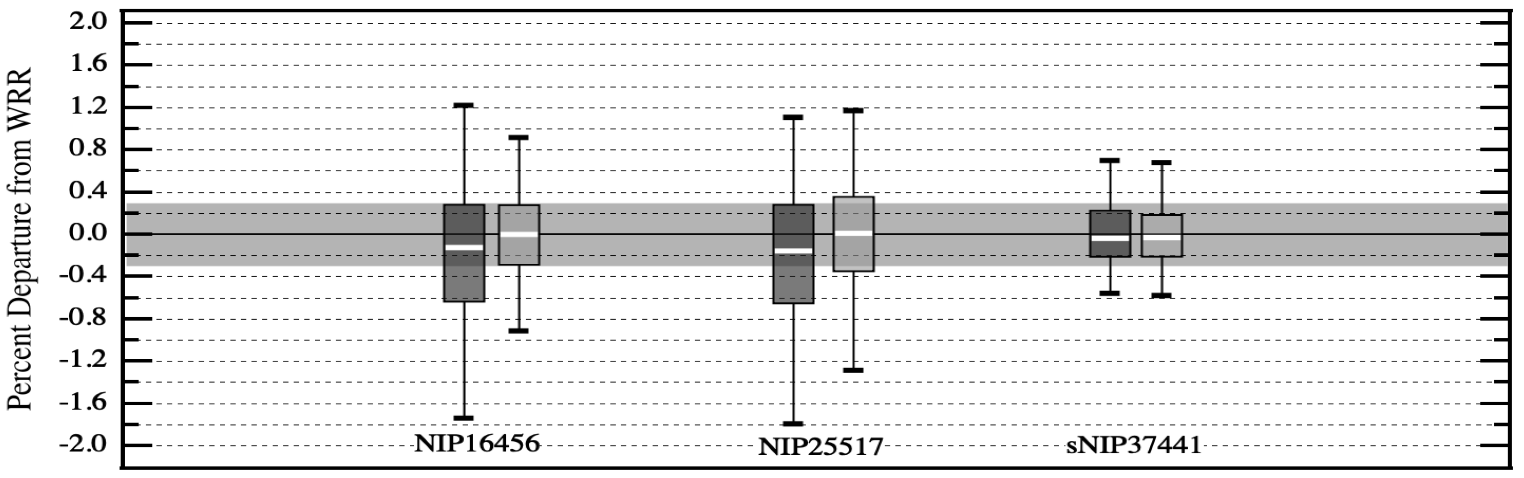
Based on these results the calibration of pyrheliometer should take into account the temperature and the angle of irradiance as well instead of relying on a single calibration factor. This can significantly improve the accuracy. This is illustrated in Figure 7. A data set was collected using a group of three working class pyrheliometers in use for decades at a WMO Region IV RRC (Regional Radiation Center) located at the NOAA/Earth Systems Research Laboratory in Boulder, Colorado. One minute averages of data sampled at one hertz over the time period from 16 May–12 August, 2013 were used to create a data set for analysis. Clear sky periods were chosen and no lower limits were imposed on irradiance values (An IPC only uses irradiance values above 700 watts/sq.m). All solar zenith angles were used for the analysis subject to a constraint that the skies were categorized as clear. A total of 14914 one minute averages were used in the analysis. The darker shaded box and whisker plots summarize residuals after subtracting the pyrheliometer irradiances computed using its assigned responsivity value from the surrogate WRR reference. The lighter shaded box plots summarize the residuals after fitting the three parameter linear model using 8 monomials. There is measurable reduction in the uncertainty.
4. Conclusion and Outlook
The precise estimation of solar irradiation is a key factor for climate modelling. The measurements are challenging due to a wide variety of measurement conditions, the need for stability on an absolute scale and the high precision requirements. The present results - based on an exhaustive Bayesian model comparison on more than different models- indicate that with relatively minor changes to the calibration protocol the achievable measurement accuracy can be significantly increased. It is highly beneficial to consider also the temperature and the angle of incidence for the calibration of the devices, improving the accuracy by more than 20% on the devices. Some further improvements appear possible: The data were analyzed as provided without any preprocessing. The residuals, however, display the presence of a small fraction of outliers which are not in agreement with the Gaussian likelihood used for the analysis. This may distort the estimate of the best fit parameters. Thus the application of a robust estimation method may improve the accuracy of the measurements even further. It could also be of interest to check if additional factors (besides temperature and angle) affect the device performance. And finally it may also be worthwhile - besides a self-consistent estimation of - to validate the estimated evidence values for the selected best fit models using thermodynamic integration or nested sampling as function of expansion order to check for a potential bias in the MAP based estimation of the evidence.
Author Contributions
D.W.N. performed the experiments and provided the data; U.v.T. analyzed the data and contributed analysis tools. The paper was written jointly.
Conflicts of Interest
The authors declare no conflict of interest.
References
- Fröhlich, C. History of Solar Radiometry and the World Radiometric Reference. Metrologia 1991, 28, 111–115. [Google Scholar] [CrossRef]
- Latimer, J. On the Angström and Smithsonian absolute pyrheliometric scales and the International Pyrheliometric Scale 1956. Tellus 1973, 15, 586–592. [Google Scholar]
- Hickey, J. Laboratory Methods of Experimental Radiometry Including Data Analysis. Adv. Geophys. 1970, 14, 227–267. [Google Scholar]
- Smithsonian Institution Radiation Biology Laboratory. In Proceedings of the Symposium on Solar Radiation Measurements and Instrumentation, Washington, DC, USA, 13–15 November 1973.
- Brusa, R.; Fröhlich, C. Realisation of the Absolute Scale of Total Irradiance; Technical Report; Swiss Meteorological Institute: Zürich, Switzerland, 1975. [Google Scholar]
- Fröhlich, C. World Radiometric Reference, Final Report; Technical Report WMO 490; World Meteorological Organization: Geneva, Switzerland, 1977. [Google Scholar]
- Finsterle, W. The International Pyrheliometer Comparison, Final Report; Technical Report WMO IOM 124; World Meteorological Organization: Davos, Switzerland, 2016. [Google Scholar]
- Nelson, D. The NOAA Climate Monitoring and Diagnostic Laboratory Solar Radiation Facility; Technical Report Technical Memorandum OAR CMDL-15; Climate Monitoring and Diagnostics Laboratory: Boulder, CO, USA, 2000. [Google Scholar]
- Kendall, J.; Burdahl, C. Two Blackbody Radiometers of High Accuracy. J. Appl. Opt. 1970, 9, 1082–1091. [Google Scholar] [CrossRef] [PubMed]
- Brusa, R.; Fröhlich, C. Absolute radiometers (PMO6) and their experimental characterisation. J. Appl. Opt. 1986, 25, 4173–4180. [Google Scholar] [CrossRef] [PubMed]
- Romero, J.; Fox, N.P.; Fröhlich, C. First compariosn of the solar and SI Radiometric Scale. Metrologia 1991, 28, 125–128. [Google Scholar] [CrossRef]
- Romero, J.; Fox, N.P.; Fröhlich, C. Improved Comparison of the World Radiometric Reference and the SI Radiometric Scale. Metrologia 1995, 32, 523–524. [Google Scholar] [CrossRef]
- Romero, J.; Fox, N.P.; Fröhlich, C. Maintenance of the World Radiometric Reference; Technical Report International Pyrheliometer Comparison IPCVIII: Working Report 188; Swiss Meteorological Organization: Zurich, Switzerland, 1996. [Google Scholar]
- Finsterle, W.; Blattner, P.; Moebus, S.; Rüedi, I.; Wehrli, C.; White, M.; Schmutz, W. Third comparison of the World Radiometric Reference and the SI radiometric scale. Metrologia 2008, 45, 377–381. [Google Scholar] [CrossRef]
- Fehlmann, A. Metrology of Solar Irradiance. Ph.D. Thesis, University of Zurich, Zurich, Switzerland, 2011. [Google Scholar]
- Kopp, G.; Fehlmann, A.; Finsterle, W.; Harber, D.; Heuerman, K.; Willson, R. Total solar irradiance data record accuracy and consistency improvements. Metrologia 2012, 49, S29–S33. [Google Scholar] [CrossRef]
- Suter, M. Advances in Solar Radiometry. Ph.D. Thesis, University of Zurich, Zurich, Switzerland, 2014. [Google Scholar]
- Reda, I.M.; Dooraghi, M.R.; Andreas, A.M.; Grobner, J.; Thomann, C. NREL Comparison Between Absolute Cavity Pyrgeometers and Pyrgeometers Traceable to World Infrared Standard Group and the InfraRed Integrating Sphere; Technical Report NREL/TP-1900-72633; National Renewable Energy Laboratory: Golden, CO, USA, 2018. [Google Scholar] [CrossRef]
- von der Linden, W.; Dose, V.; von Toussaint, U. Bayesian Probability Theory: Applications in the Physical Sciences; Cambridge University Press: Cambridge, UK, 2014. [Google Scholar] [CrossRef]
- Press, W.H.; Teukolsky, S.A.; Vetterling, W.T.; Flannery, B.P. Numerical Recipes 3rd Edition: The Art of Scientific Computing, 3rd ed.; Cambridge University Press: Cambridge, UK, 2007. [Google Scholar]
Figure 1.
Left panel [8] shows efforts to establish a radiometric scale during the 20th century. The shaded band marks the adoption of the WRR. Relative relationships of the scales with respect to the current WRR are shown. Right panel illustrates the results for three cavities from WMO Region IV (North American Region) which participated in IPC-XII in 2015. Box plot data: box midlines are medians, box lower and upper boundaries are at the 25th and 75th percentiles and the box whisker caps are at the 2nd and 98th percentiles. Shaded bands in both panels denote the accepted uncertainty in the WRR. The scale in righthand panel is expanded by a factor of 12 with respect to panel on left.
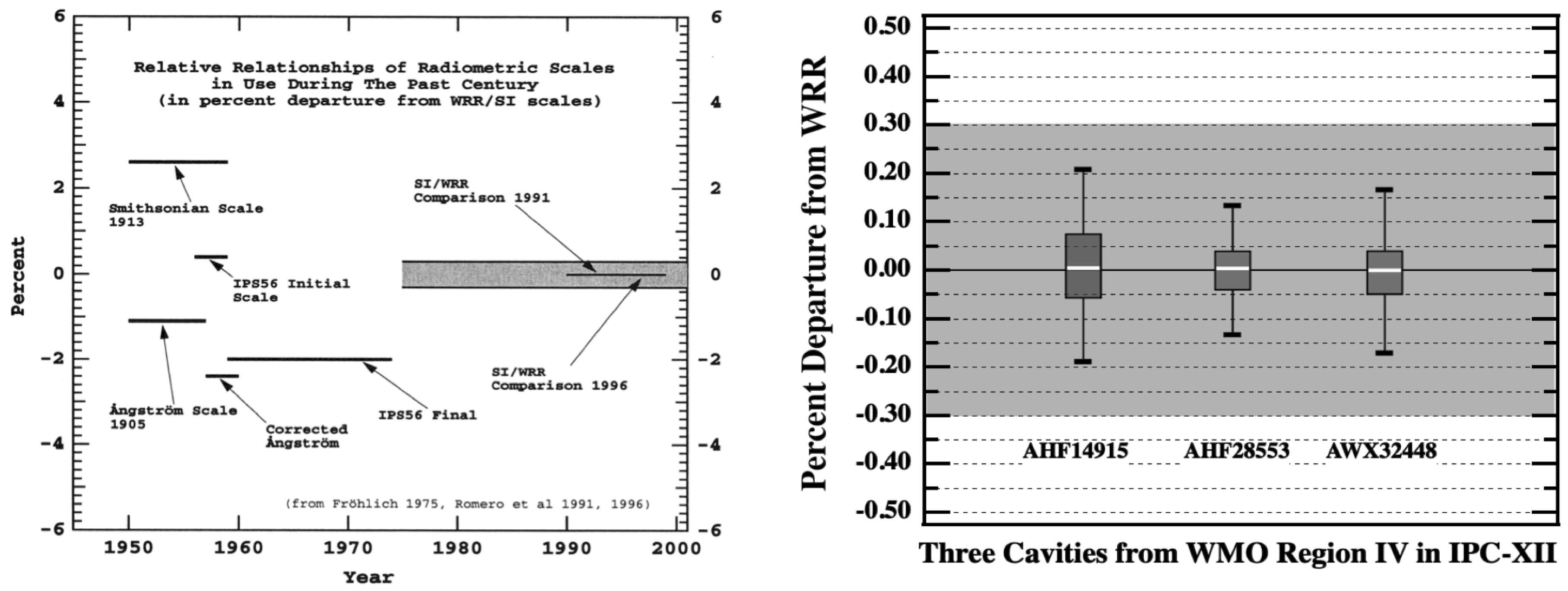
Figure 2.
Box and whisker plots from IPC-XII Results for three North American Region cavity type pyrheliometers and a group of three working class pyrheliometers typically used at monitoring sites in WMO regions. Whisker caps are at 2nd and 98th percentiles. Box boundaries at 25th and 75th percentiles and median. Shaded band is stated uncertainty of the WRR. Precision losses in WRR ratios can range from factors of ten up to forty [7].
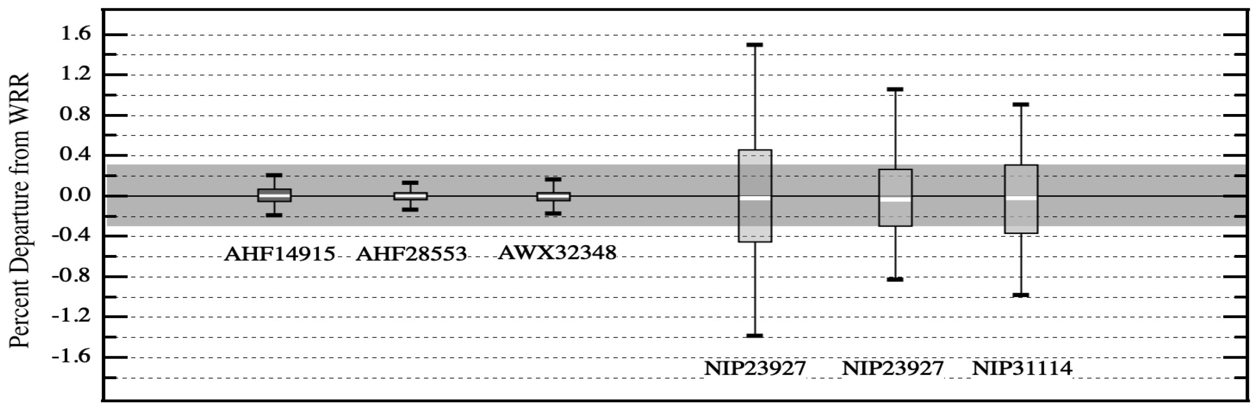
Figure 3.
Results for three North American Region cavity type pyrheliometers. Darker shaded box plot data: IPC-XII 2015. Lighter shaded box plot data: NPC-2018. The shaded band across the graph is the historical assigned uncertainty of the WRR. Box and whisker information is the same as in Figure 1 and Figure 2.
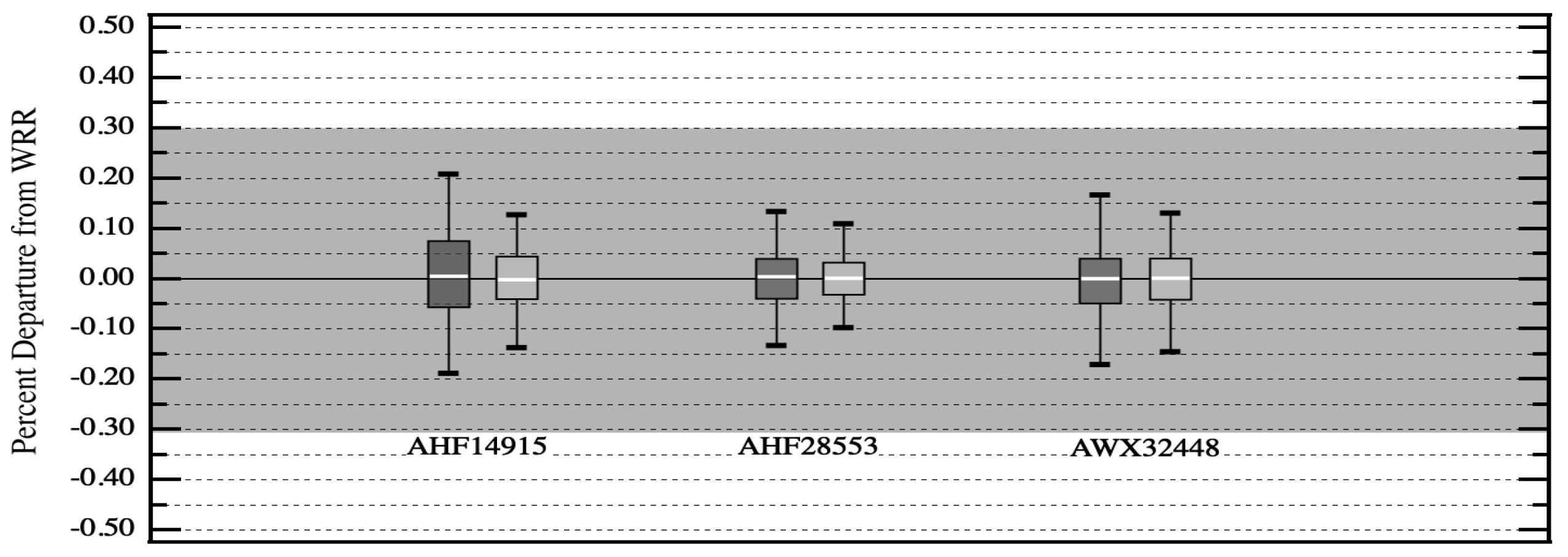
Figure 4.
Results for three working class pyrheliometers used to collect clear sky solar irradiance data from 16 May 2013 to 12 August 2013. Sampling rate was 1 hertz and data were processed into one minute averages. A total of 14914 data points are included in the data set. The solid lines are given by linear regression of to the measured data for each of the three devices.
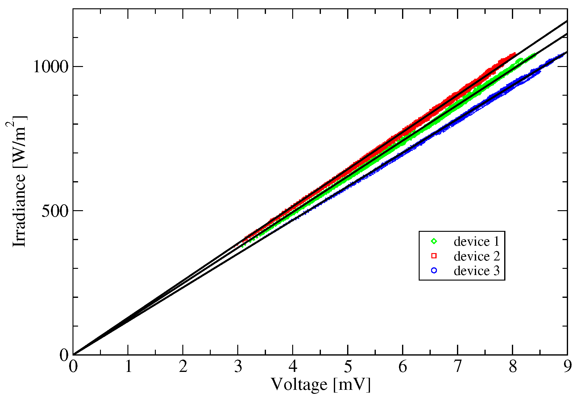
Figure 5.
Panel (a) displays the difference between the data and the linear model for one of the data sets displayed in Figure 4. Panel (b) provides the residuum if instead of a model linear in the measured voltage a quadratic relationship is being assumed. The overall magnitude of the residuum in panel (b) is visibly smaller compared with panel (a). However, if the residuum is plotted as function of the device temperature (panel (c)) again a non-stochastic behavior is evident. Instead, panel (d) displays a bivariate regression function i.e., a sum of a quadratic function of the voltage and a quadratic function of the temperature T appears to capture the data reasonably well. The resulting residuum shows no clear non-stochastic behavior.
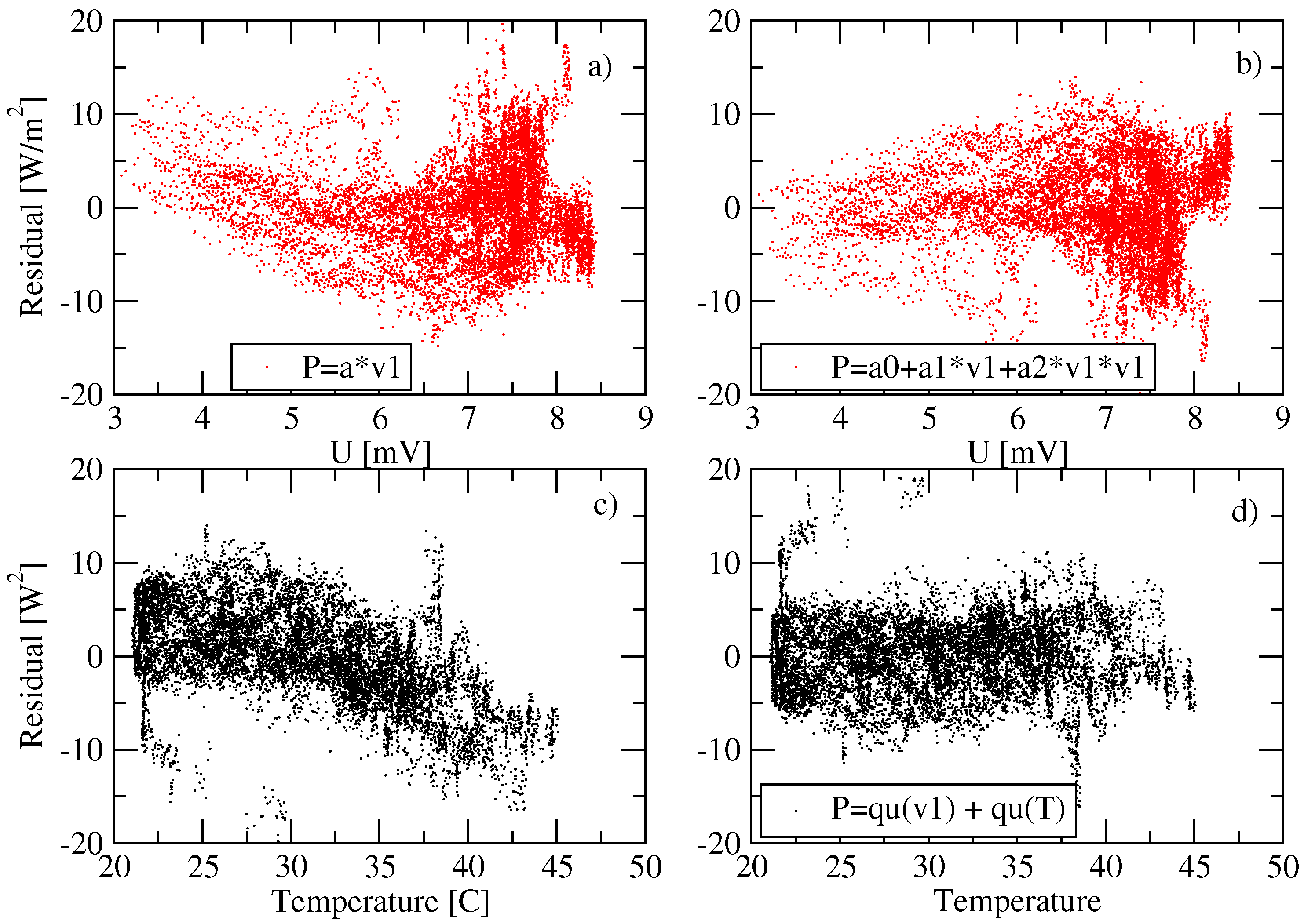
Figure 6.
Misfit and evidence as function of the number of parameters. For each number of parameters the corresponding best fit is provided. On the left hand ordinate the misfit (-value) between data and model is given. On the ordinate on the right hand side the logarithm of the model evidence is given. Higher values indicate a more probable model. As can be clearly seen from both misfit and model evidence the commonly used 1 parameter regression is inadequate. The evidence obtains nearly identical peak value maxima for 7 and 9 parameters where also the improvement for the -values levels off.
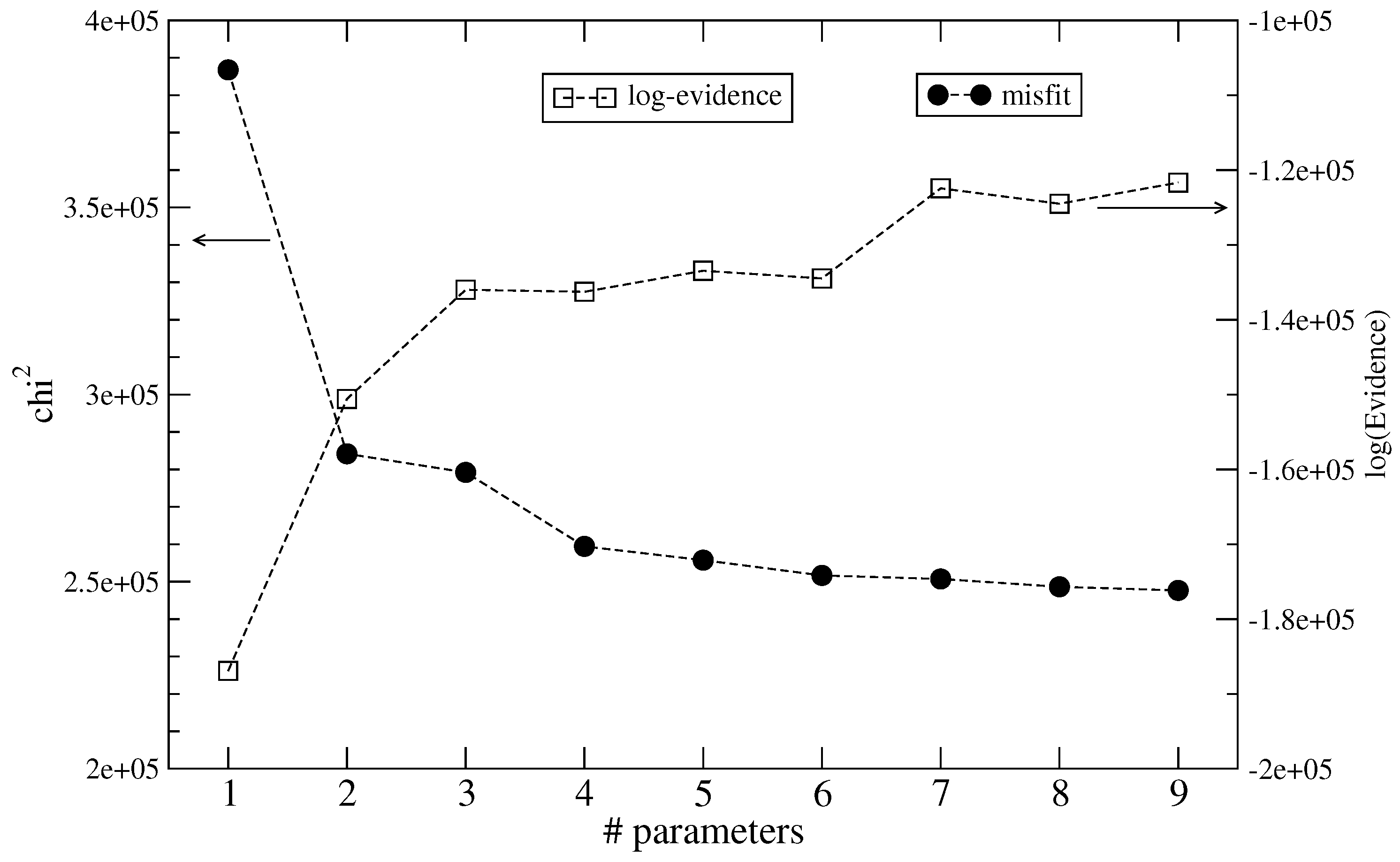
Figure 7.
Results for three working class pyrheliometers used to collect clear sky solar irradiance data from 16 May 2013 to 12 August 2013. Sampling rate was 1 hertz and data were processed into one minute averages. A total of 14914 data points are included in the data set. Solar zenith angle range: 16–84 degrees Irradiance range: 375–1050 watts per square meter. Darker shaded boxes are residual summaries of ratio responsivity scaling. The lighter shaded boxes are residual summaries of a linear model scaling of pyrheliometer outputs. Box and whisker information is the same as in Figure 1, Figure 2 and Figure 3.
© 2020 by the authors. Licensee MDPI, Basel, Switzerland. This article is an open access article distributed under the terms and conditions of the Creative Commons Attribution (CC BY) license (http://creativecommons.org/licenses/by/4.0/).
Share and Cite
MDPI and ACS Style
Nelson, D.W.; Toussaint, U.v. Radiometric Scale Transfer Using Bayesian Model Selection. Proceedings 2019, 33, 32. https://doi.org/10.3390/proceedings2019033032
AMA Style
Nelson DW, Toussaint Uv. Radiometric Scale Transfer Using Bayesian Model Selection. Proceedings. 2019; 33(1):32. https://doi.org/10.3390/proceedings2019033032
Chicago/Turabian StyleNelson, Donald W., and Udo von Toussaint. 2019. "Radiometric Scale Transfer Using Bayesian Model Selection" Proceedings 33, no. 1: 32. https://doi.org/10.3390/proceedings2019033032