Improving Energy Savings of a Library Building through Mixed Mode Hybrid Ventilation †


Abstract
:1. Introduction
2. Methodology
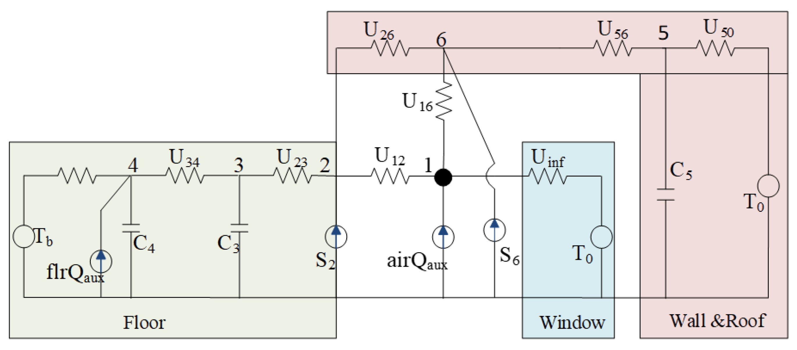
Thermal Network
- Ai: area of surface i (m2);
- hc,i: convective heat transfer coefficient of surface i (Wm−2K−1);
- σ: Stefan-Boltzmann constant (Wm−2K−4);
- Fi,j*: radiative exchange factor between surfaces i and j;
- Tm: mean surface temperature (°C);
- Ui,j: thermal conductance between nodes i and j (WK−1)
- Qi: heat at node i (due to internal heat gain, solar heat gain or auxiliary heat) (W)
- kp: proportional control
- Tsp: set-point temperature (°C)
- Ti: temperature at node i (°C)
- Ci: thermal capacitance of node i (JK−1)
- Δt: simulation time step (s)
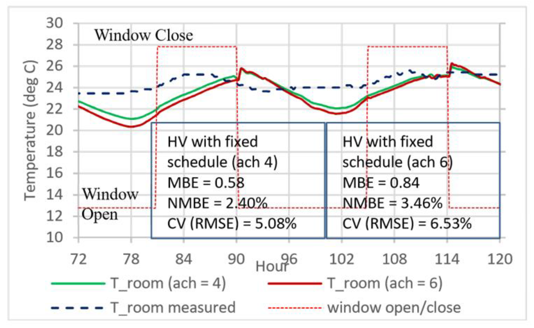
3. Model Verification
4. Simulation Strategies
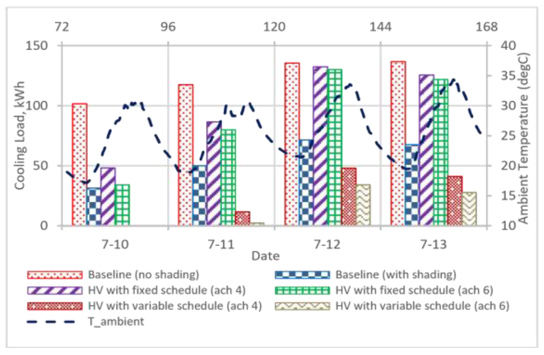
5. Results and Discussion
6. Conclusions
Author Contributions
Acknowledgments
Conflicts of Interest
References
- Hu, J.; Karava, P. Model predictive control strategies for buildings with mixed-mode cooling. Build. Environ. 2014, 71, 233–244. [Google Scholar] [CrossRef]
- Brager, G.; Borgeson, S.; Lee, Y. Summary Report: Control Strategies for Mixed-Mode Buildings; Technical Report for UC Berkeley; Center for the Built Environment: Berkeley, CA, USA, 2007. [Google Scholar]
- May-Ostendorp, P.; Henze, G.P.; Corbin, C.D.; Rajagopalan, B.; Felsmann, C. Model-predictive control of mixed-mode buildings with rule extraction. Build. Environ. 2011, 46, 428–437. [Google Scholar] [CrossRef]
- Dermardiros, V.; Athienitis, A.K.; Bucking, S. Energy performance, comfort and lessons learned from an instituitional building designed for net-zero energy. ASHRAE Trans. 2019, 125, 682–695. [Google Scholar]
- Athienitis, A.K. Building thermal analysis. In Electronic MathCAD Book; MathSoft Inc.: Boston, MA, USA, 1994. [Google Scholar]
- Derakhtenjani, A.S.; Athienitis, A.K. A study of the effect of model resolution in analysis of building thermal dynamics. In Proceedings of the 15th IBPSA Conference, San Francisco, CA, USA, 7–9 August 2017; p. 16221633. [Google Scholar]
- Athienitis, A.K.; Stylianou, M.; Shou, J. A methodology for building thermal dynamics studies and control applications. ASHRAE Trans. 1990, 96, 839–848. [Google Scholar]
- Cheng, H. Evaluating the Performance of Natural Ventilation in Buildings Through Simulation and On-Site Monitoring. Master’s Thesis, Massachusetts Institute of Technology, Cambridge, MA, USA, 2011. [Google Scholar]


| No. | Description |
|---|---|
| Node #1 | Room Air |
| Node #2 | Interior surface of the radiant floor |
| Nodes #3 & #4 | Inside radiant floor (discretized into two control volumes, C3 and C4) |
| Node #5 | Inside walls and roof (considered as one control volume, C5) |
| Node #6 | Node at the interior surface of walls and roof (considered as one node) |
| U12, U16 | Convective conductance between air node and interior surfaces |
| U26 | Radiative conductance between interior surfaces |
| U23, U34, U56 | Conductive conductance of surfaces due to thermal mass |
| Uinf | Conductance due to infiltration through windows |
| T0, Tb | Ambient and basement temperature |
| Tsp_air, Tsp_floor | Set-point temperature of room air and radiant floor |
| S2, S6 | 70% and 30% of total solar gain absorbed by the floor and the remaining surfaces |
| AirQaux, FlrQaux | Auxiliary heating/cooling source for room air and radiant floor |
| Cooling Mode | Set-Point Temperature Tsp | Motorized Window (Open/Closed) | |
|---|---|---|---|
| Baseline (no shading) | 100% mechanical cooling | Tsp_air = 24 °C Tsp_floor = 23 °C | CLOSED |
| Baseline (shading 11.00 a.m.–4.00 p.m.) | 100% mechanical cooling | Tsp_air = 24 °C Tsp_floor = 23 °C | CLOSED |
| HV with fixed schedules (4 ach) | Mixedmode cooling | Tsp_air = 24 °C Tsp_floor = 23 °C | CLOSED (9.00 a.m. to 6.00 p.m.); Otherwise OPEN |
| HV with fixed schedules (6 ach) | Mixedmode cooling | Tsp_air = 24 °C Tsp_floor = 23 °C | CLOSE (9.00 a.m. to 6.00 p.m.); Otherwise OPEN |
| HV with variable schedules (4 ach) | Mixedmode cooling | Tsp = 24 °C (8.00 a.m. to 4.00 p.m.) Tsp = 26 °C (remaining hr) | OPEN (Tamb ≈ 15 °C to 25 °C) |
| HV with variable schedules (6 ach) | Mixedmode cooling | Tsp = 24 °C (8.00 a.m. to 4.00 p.m.) Tsp = 26 °C (remaining hr) | OPEN (Tamb ≈ 15 °C to 25 °C) |
Disclaimer/Publisher’s Note: The statements, opinions and data contained in all publications are solely those of the individual author(s) and contributor(s) and not of MDPI and/or the editor(s). MDPI and/or the editor(s) disclaim responsibility for any injury to people or property resulting from any ideas, methods, instructions or products referred to in the content. |
© 2019 by the authors. Licensee MDPI, Basel, Switzerland. This article is an open access article distributed under the terms and conditions of the Creative Commons Attribution (CC BY) license (https://creativecommons.org/licenses/by/4.0/).
Share and Cite
Sultana, S.; Athientis, A.K.; Zmeureanu, R.G. Improving Energy Savings of a Library Building through Mixed Mode Hybrid Ventilation. Proceedings 2019, 23, 3. https://doi.org/10.3390/proceedings2019023003
Sultana S, Athientis AK, Zmeureanu RG. Improving Energy Savings of a Library Building through Mixed Mode Hybrid Ventilation. Proceedings. 2019; 23(1):3. https://doi.org/10.3390/proceedings2019023003
Chicago/Turabian StyleSultana, Sormin, Andreas K. Athientis, and Radu G. Zmeureanu. 2019. "Improving Energy Savings of a Library Building through Mixed Mode Hybrid Ventilation" Proceedings 23, no. 1: 3. https://doi.org/10.3390/proceedings2019023003
APA StyleSultana, S., Athientis, A. K., & Zmeureanu, R. G. (2019). Improving Energy Savings of a Library Building through Mixed Mode Hybrid Ventilation. Proceedings, 23(1), 3. https://doi.org/10.3390/proceedings2019023003