Early Detection of Damages Based on Comprehensive Theory of Deformation and Fracture ^†

Abstract

Numerical studies have been conducted based on the recently published Deformation Field Theory. Effects of pulling rates on displacement waves and volume expansion waves are analyzed in a finite element model (FEM) of a solid experiencing a uni-axial tensile load. Without relying on empirical data, the model’s numerical results demonstrate empirically known concepts that a fracture occurs more easily when the pulling rate is high, and the direction of external load is reversed.

1. Introduction

The majority of conventional fracture mechanics analyses begin with a crack-tip already introduced in the model or specimen [1,2]. In strength of materials, stress strain curves are designed mostly from empirical methods often associated with a specific strain rate. Neither approach predicts where and when a fracture will occur in a solid, until a crack appears. However, Deformation Field Theory [3,4] provides a physics based theoretical framework that describes all stages of deformation comprehensively. Within this same theoretical foundation, Deformation Field Theory derives field equations that describe the local deformation behavior as wave dynamics. Thus, we can describe deformation in solids, in terms of wave dynamics of deformation fields. When studying deformation as waves propagating through materials, we can provide a thorough analysis of the translational and rotational dynamics a solid is experiencing.

In this study we use Deformation Field Theory to model the effect of pulling rates on the deformation behavior of a specimen. Empirically it is well known that the pulling rate alters the ductile-brittle transition behavior of steel [5,6]. We propose that when a solid is experiencing a uni-axial tensile load at a strain rate, such as $1\times {10}^{-3}$ s⁻¹, a faster pulling rate causes the material to undergo more concentrated volume expansion. From the Deformation Field Theory perspective, the deformation wave velocity, of a solid experiencing plastic deformation, does not depend on the pulling rate. Consequently, if the pulling rate is slow the material has time to redistribute the stress via wave propagation. Conversely, if the pulling rate is fast the material does not have time to redistribute the stress via wave propagation, leading to fracture more easily.

We developed a finite element model (FEM) of a solid experiencing a uni-axial tensile load, studying three pulling cases; intermediate ($1\times {10}^{-3}$ s⁻¹ in strain rate) and comparatively fast and slow. Using the field equations of Deformation Field Theory, we derived an equation of motion, expressed it in the form of a wave equation, and solved it as a two-dimensional partial differential equation, over the area of the modeled specimen. We introduced a new parameter, $\alpha$, to describe the degree of plastic deformation [7]. Without using empirical data acquired from stress strain analysis, our model can demonstrate deformation concepts already known in a phenomenological sense. Specifically, fast pulling tends to tear solid objects more easily and often a fracture occurs when the direction of the applied force is reversed.

2. Field theory of Deformation and Fracture

2.1. Field Equations

Details of the present field theory can be found elsewhere [3,4]. In short, this theory describes all stages of deformation based on two postulates. The first postulate is that at any stage of deformation it is possible to find local regions in solids where the deformation obeys the law of liner elasticity (Hooke’s law). Those local regions are called the deformation structural elements. The second postulate is that nonlinear dynamics in the plastic regime can be formulated through a compensation field that logically connects deformation structural elements so that Hooke’s law can be satisfied at the global level. The irreversibility in the plastic regime is described through energy dissipative interaction between the deformation structural element and the compensation field. Fracture is characterized as the final stage of deformation where the compensation field is unable to connect deformation structural elements, and therefore the solid is no longer a continuum medium.

Hooke’s law is an orientation preserving law [8] as the elastic force and resultant displacement are parallel to each other. Therefore, in order to describe deformation with Hooke’s law at the global level, it is necessary to align all deformation structural elements in the same direction. The role of the compensation field is to make this orientation recovering alignment. This effect is conveniently expressed as a vector potential. With this formalism, solids under deformation can be viewed as being made up with a number of elastic entities connected with the vector potential.

The present field theory identifies Lagrangian associated with the local elastic energy and potential energy associated with the vector potential. By applying the Lagrangian principle, the theory derives the following set of field equations.

$$\nabla ·\overrightarrow{v}=-j^0,$$

(1)

$$\nabla \times \overrightarrow{v}=\frac{\partial \overrightarrow{\omega }}{\partial t},$$

(2)

$$\nabla \times \overrightarrow{\omega }=-\frac{1}{c^2}\frac{\partial \overrightarrow{v}}{\partial t}-\overrightarrow{j}.,$$

(3)

$$\nabla ·\overrightarrow{\omega }=0.$$

(4)

Apparently, the above field equations yield wave solutions. This is the source of the wave dynamics of deformation fields. In the field equations, $\overrightarrow{v}$ is the temporal derivative of displacement $\overrightarrow{\xi }$ at a given point in the global coordinate system ($\overrightarrow{v}=\overrightarrow{\dot{\xi }}$), $\overrightarrow{\omega }$ is the rotation ($\overrightarrow{\omega }=\nabla \times \overrightarrow{\xi }$), and $c$ is the wave velocity. $j^0$ and $\overrightarrow{j}$ are the quantities that describe temporal and spatial interaction of the local elastic dynamics with the compensation field. Equation (3) can be put in the following form, which explicitly indicates that this equation is in fact the equation of motion for the unit volume whose mass is $\rho$.

$$\rho \frac{{\partial }^2\overrightarrow{\xi }}{\partial t^2}=-G\left(\nabla \times \overrightarrow{\omega }\right)-G\overrightarrow{j}.$$

(5)

In the form of Equation (5), $G\left(\nabla \times \overrightarrow{\omega }\right)$ and $G\overrightarrow{j}$ can be interpreted as representing shear and longitudinal resistant forces that the solid exerts in response to the external load. Each regime of deformation can be characterized by a specific form of the resistant force as indicated in

Table 1. Resistive force for each regime of deformation.

Deformation Regime	Resistive Force Expression
Linear elastic	$\nabla \left(\lambda +G\right)\left(\nabla ·\overrightarrow{\xi }\right)$
Elasto-plastic 1	$-G\left(\nabla \times \overrightarrow{\omega }\right)-{\sigma }_0\rho \left(\nabla ·\overrightarrow{v}\right)\overrightarrow{v}+\nabla \left(\lambda +G\right)\left(\nabla ·\overrightarrow{\xi }\right)$
Elasto-plastic 2	$-G\left(\nabla \times \overrightarrow{\omega }\right)-{\sigma }_0\rho \left(\nabla ·\overrightarrow{v}\right)\overrightarrow{v}$
Pre-fracture 1	$E\left(\frac{{\partial }^4{\xi }_s}{\partial x_s{}^4}\right)d{x}_s{}^2-{\sigma }_0\rho v_s\frac{\partial v_s}{\partial x_s}$

¹ The first term comes from a higher order term of the Lagrangian. $E$ is the Young’s modulus.

, and briefly described as follows.

• Linear elastic regime

For this regime, material rotation $\overrightarrow{\omega }$ represents rigid-body rotation. In other words, the entire object is represented by the same $\overrightarrow{\omega }$ vector, hence, $\nabla \times \overrightarrow{\omega }=0$. The elastic force is proportional to the volume expansion via the Lamé’s parameters $\lambda$ and $G$.

2.

Elasto-plastic regime 1

In this regime, the number and size of defects become significant, making different parts of the object undergo different rotations. Consequently, $\nabla \times \overrightarrow{\omega }\ne 0$. In addition, these defects move causing friction against surrounding atoms. This energy dissipative force is expressed via a material constant, ${\sigma }_0$, as ${\sigma }_0\rho \left(\nabla ·\overrightarrow{v}\right)\overrightarrow{v}$. The solid is still under the influence of elastic force, $\nabla \left(\lambda +G\right)\left(\nabla ·\overrightarrow{\xi }\right)$.

3.

Elasto-plastic regime 2

When deformation advances to the next level, the number and size of defects become so high that the solid is no longer under the influence of elastic force, $\nabla \left(\lambda +G\right)\left(\nabla ·\overrightarrow{\xi }\right)$. However, it is still influenced by rotational elastic force, $G\left(\nabla \times \overrightarrow{\omega }\right)$.

4.

Pre-fracture regime

When deformation develops further, the shear stress becomes so significant that a so-called shear band appears at the location of maximum shear stress [3]. At this stage, $\nabla \times \overrightarrow{\omega }$ becomes uni-directional . The elastic force term is due to a higher order term of the Lagrangian, representing elastic energy. Note that the equation of motion yields solitary waves in this regime.

2.2. Wave Equations

From Table 1, the equation of motion (5) for Elasto-plastic 1 regime can be put as follows.

$$\frac{{\partial }^2\overrightarrow{\xi }}{\partial t^2}+{\sigma }_0\left(\nabla ·\overrightarrow{v}\right)\frac{\partial \overrightarrow{\xi }}{\partial t}=-\frac{G}{\rho }\left(\nabla \times \omega \right)+\frac{\lambda +G}{\rho }\nabla \left(\nabla ·\overrightarrow{\xi }\right).$$

(6)

Similarly, the equation of motion for Elasto-plastic 2 becomes

$$\frac{{\partial }^2\overrightarrow{\xi }}{\partial t^2}+{\sigma }_0\left(\nabla ·\overrightarrow{v}\right)\frac{\partial \overrightarrow{\xi }}{\partial t}=-\frac{G}{\rho }\left(\nabla \times \overrightarrow{\omega }\right).$$

(7)

The last term of Equation (6) indicates that as deformation develops from Elasto-plastic 1 to Elasto-plastic 2, the coefficient of the linear elastic force term changes from $\lambda +G$ to 0. This indicates that the degree of plastic deformation cab be expressed by parameter $\alpha$ defined as follows.

$$\frac{{\partial }^2\overrightarrow{\xi }}{\partial t^2}+{\sigma }_0\left(\nabla ·\overrightarrow{v}\right)\frac{\partial \overrightarrow{\xi }}{\partial t}=-\frac{G}{\rho }\left(\nabla \times \omega \right)+\alpha \frac{G}{\rho }\nabla \left(\nabla ·\overrightarrow{\xi }\right).$$

(8)

Here, $\alpha$ changes from $\alpha =\left(\lambda +G\right)/G$ for Elasto-plastic 1 to $\alpha =0$ for Elasto-plastic 2.

With the identity $\nabla \times \overrightarrow{\omega }=\nabla \left(\nabla ·\overrightarrow{\xi }\right)-{\nabla }^2\overrightarrow{\xi }$, $\overrightarrow{\omega }$ can be eliminated from Equation (8) as follows.

$$\frac{{\partial }^2\overrightarrow{\xi }}{\partial t^2}+{\sigma }_0\left(\nabla ·\overrightarrow{v}\right)\frac{\partial \overrightarrow{\xi }}{\partial t}=\frac{G}{\rho }{\nabla }^2\overrightarrow{\xi }-\frac{G}{\rho }\nabla \left(\nabla ·\overrightarrow{\xi }\right)+\alpha \frac{G}{\rho }\nabla \left(\nabla ·\overrightarrow{\xi }\right)=\frac{G}{\rho }{\nabla }^2\overrightarrow{\xi }+\left(\alpha -1\right)\frac{G}{\rho }\nabla \left(\nabla ·\overrightarrow{\xi }\right).$$

(9)

3. Modeling

3.1. Partial Differential Equation

In the present study, the above equation of motion is solved as a FEM of two-dimensional, partial differential equation. Equation (9) can be viewed as a wave equation of the following form.

$$\frac{{\partial }^2\overrightarrow{\xi }}{\partial t^2}+{\sigma }_0\left(\nabla ·\overrightarrow{v}\right)\frac{\partial \overrightarrow{\xi }}{\partial t}-\frac{G}{\rho }{\nabla }^2\overrightarrow{\xi }=\left(\alpha -1\right)\frac{G}{\rho }\nabla \left(\nabla ·\overrightarrow{\xi }\right).$$

(10)

Here ${\sigma }_0\left(\nabla ·\overrightarrow{v}\right)$ can be viewed as a damping coefficient, $G/\rho$ as the square of the wave velocity, and $\left(\alpha -1\right)\left(G/\rho \right)\nabla \left(\nabla ·\overrightarrow{\xi }\right)$ as the source term. Based on the argument made above, the transition from Elasto-plastic 1 to Elasto-plastic 2 in association with the change in $\alpha$ can be viewed as the corresponding change in the coefficient of the source term.

For Elasto-plastic 1, $\alpha G=\lambda +G$. According to continuum mechanics, $\lambda$ and $G$ are related via Poisson’s ratio, $\nu$, as $\lambda /G=2\nu /\left(1-2\nu \right)$. With a typical value $\nu =0.3$, the coefficient of the source term in Equation (10) becomes $\alpha -1=\lambda /G=1.5$. For Elasto-plastic 2, $\alpha =0$ makes the coefficient $\alpha -1=-1$. With these two coefficients, wave Equation (10) can be solved with boundary conditions.

3.2. Boundary Condition

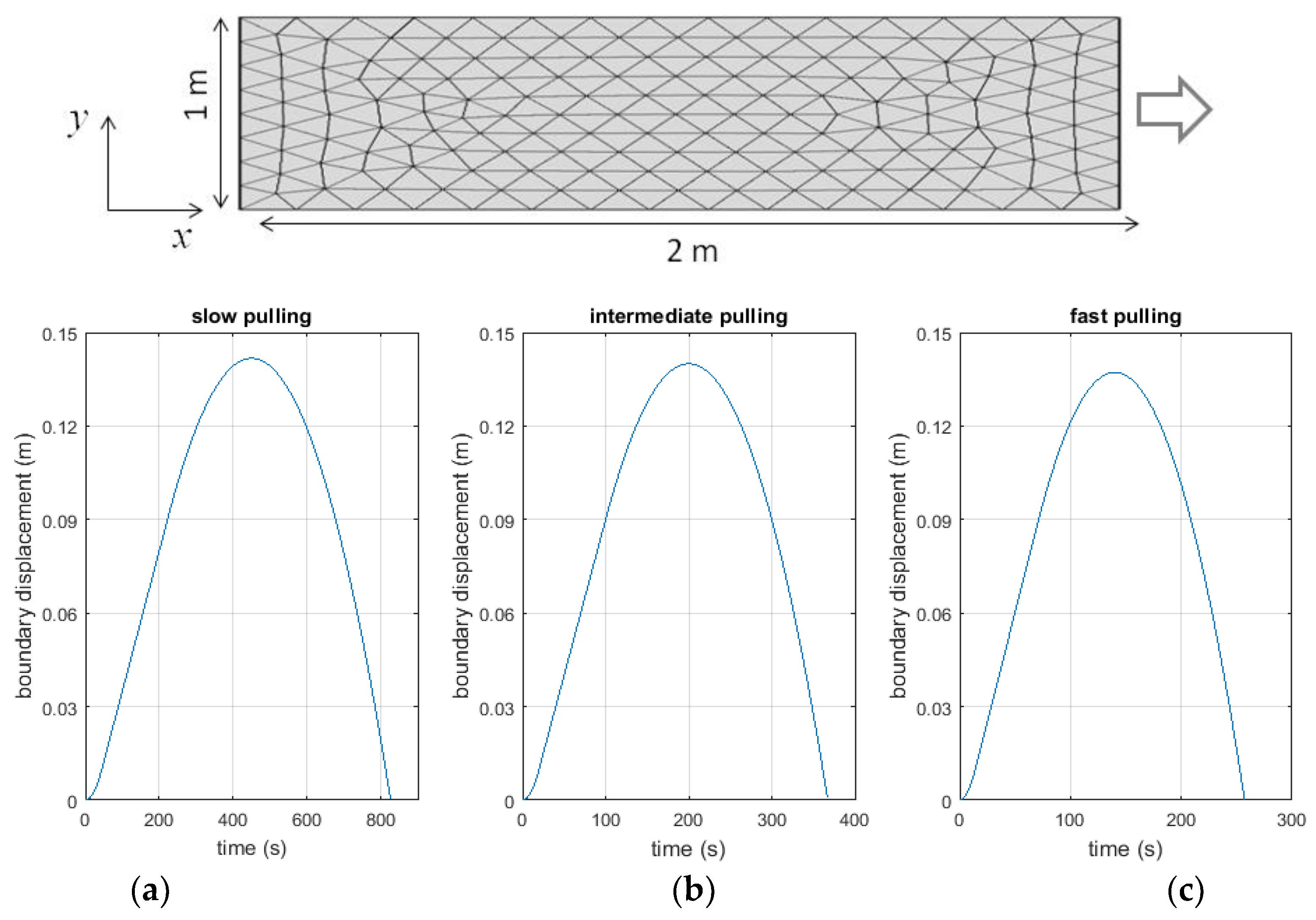
The upper illustration in Figure 1 shows the specimen with the mesh used for our FEM analysis. The left end of the planar specimen is fixed both vertically and horizontally. The right end is pulled by a tensile machine with zero vertical freedom. The top and bottom ends are assumed to be free. The lower plots in Figure 1 show the three boundary conditions used for the right end.

4. Results and Discussions

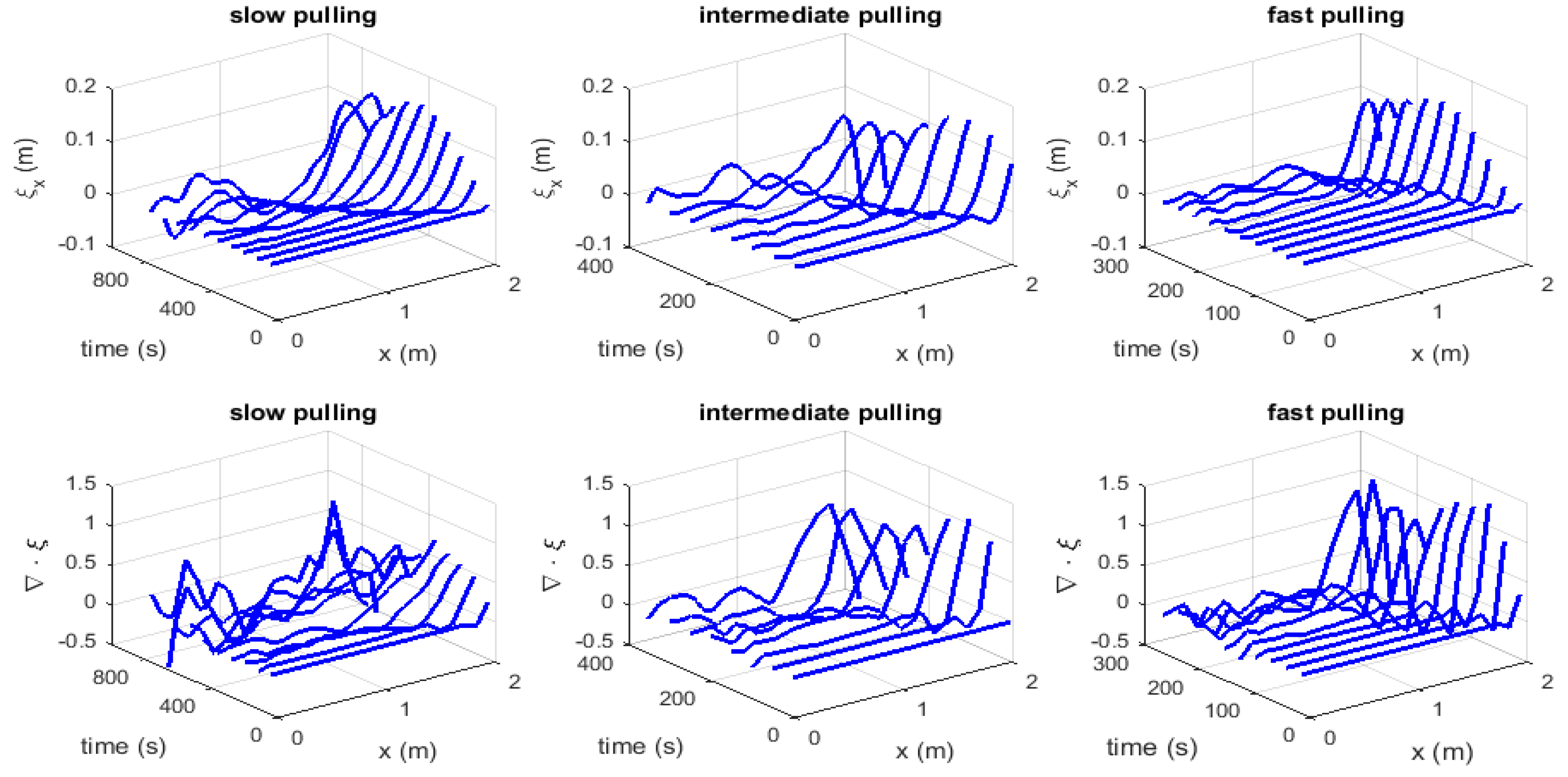
In the present study, the focus is on the effect of pulling rate on the wave behaviors for Elasto-plastic 2 ($\alpha =0$ in Equation (10)). Figure 2 shows the computed ${\xi }_x$ (the displacement component in line of the external pulling load) waves and $\nabla ·\overrightarrow{\xi }$ (volume expansion) waves for the slow (left column), intermediate (middle column) and fast (right column) pulling rates. The top graphs are the ${\xi }_x$-waves and the bottom graphs are the $\nabla ·\overrightarrow{\xi }$-waves.

The following observations can be made.

• The effect of pulling rate is more prominent in the volume expansion waves than the displacement waves. This indicates that the volume expansion part of $\nabla \times \overrightarrow{\omega }=\nabla \left(\nabla ·\overrightarrow{\xi }\right)-{\nabla }^2\overrightarrow{\xi }$ is more sensitive to the pulling rate.
• The effect of pulling rate is more prominent in the second half (the descending half of Figure 2) than the first half (the ascending half of Figure 1). Fracture is induced by strain concentration. This observation indicates that fracture occurs when the direction of the applied force is reversed. It also indicates that the deformation dynamics is more influential to strain concentration than the average strain. Notice that the pulling is symmetric in time so that the average strain is symmetric in the ascending and descending halves.
• The fast pulling case indicates more concentrated volume expansion. This can be interpreted as follows. When pulled slowly, the solid has time to redistribute the volume expansion. Conversely, when pulled fast, at a certain peak in ${\xi }_x$ or $\nabla \overrightarrow{ \xi }$ is more prominent than the others. In other words, the solid tends to have strain concentration more easily when pulled faster. This and Observation 2 are consistent with our intuition that when we try to break a solid object we tend to apply a force in one direction and reverse the direction fast.

The above observations indicate the interaction between the deformation waves and the end of the solid that the uni-axial tensile load is applied. Figure 3 shows the motion of the largest peak of the ${\xi }_x$-wave as a function of time. It is clearly seen that the wave’s motion deviates from linearity more clearly when pulled slowly and in the descending part of the pulling action. Notice that the wave Equation (10) uses a constant wave velocity ($\sqrt{G/\rho }$). Therefore, without the interaction with the pulling at the boundary, the motion of the peak should be constant. The dashed line in the middle plot of Figure 3 indicates the constant velocity.

5. Conclusions

The present study demonstrates, via wave dynamics of deformation, empirically known concepts that it is more likely fast pulling leads to a fracture and that a fracture tends to occur when the direction of the applied load changes. Although the current FEM does not model the pre-fracture regime (Table 1), it is possible to argue that the prominent peak observed in the fast pulling case transforms to a solitary wave. Deformation Field Theory predicts that a fracture occurs when and where a solitary wave stops travelling. Modeling of the transition from a continuous wave to a solitary wave and of the mechanism that makes a solitary wave stationary are two most important subjects of our future study.

References

- Anderson, T.L. Fracture Mechanics: Fundamentals and Applications, 4th ed.; CRC Press: New York, USA, 2017. [Google Scholar]
- Barsom, J.M.; Rolfe, S.T. Fracture and Fatigue Control in Structures: Applications of Fracture Mechanics, 3rd ed.; ASTM: West Conshohocken, PA, USA, 1999. [Google Scholar]
- Yoshida, S. Deformation and Fracture of Solid-State Materials: Field Theoretical Approach and Engineering Applications, 1st ed.; Springer: New York, NY, USA, 2015. [Google Scholar]
- Yoshida, S. Comprehensive description of deformation of solids as wave dynamics. Math. Mech. Complex Syst. 2015, 3, 243–272. [Google Scholar] [CrossRef]
- Barsom, J.M.; Rolfe, S.T. Effects of Temperature, Loading Rates, and Constraint. In Fracture and Fatigue Control in Structures, Applications of Fracture Mechanics, 3rd ed.; ASTM: West Conshohocken, PA, USA, 1999; pp. 95–117. [Google Scholar]
- Armstrong, R.W.; Walley, S.M. High strain rate properties of metals and alloys. Int. Mater. Rev. 2008, 53, 105–128. [Google Scholar] [CrossRef]
- Yoshida, S.; Sadeqi, S. Wave dynamics of deformation and fracture. AIP Conf. Proc. 2017, 1895, 040005. [Google Scholar] [CrossRef]
- Marsden, J.E.; Hughes, T.J.R. Mathematical Foundations of Elasticity; Prentice-Hall: Englewood Cliffs, NJ, USA, 1983. [Google Scholar]
Figure 1.
The specimen and three pulling rates used in FEM: (a) slow; (b) intermediate and (c) fast.
Figure 2.
–waves (top three plots) and –waves (bottom three plots) observed at three pulling rates: slow (left); intermediate (middle) and fast pulling rates (right).
Figure 3.
Peak location of –waves v.s. time: (a) slow; (b) intermediate and (c) fast pulling rates.