From Linear Programming Model to Mixed Integer Linear Programming Model for the Simultaneous Optimisation of Water Allocation and Reservoir Location in River Systems ^†

Abstract

The allocation of water flowing through a river-with-reservoirs system to optimally meet spatially distributed and temporally variable demands can be conceived as a Network Flow Optimisation (NFO) problem and addressed by Linear Programming (LP). In this paper we present an extension of the strategic NFO-LP model to simultaneously optimise the allocation of water and the location of one or more reservoirs. The applicability of the MILP model has been illustrated by applying it to a hypothetical river network configuration consisting of seven candidate reservoir nodes and seven demand nodes, and by comparing the outcome (water levels in selected reservoir, penalties) with the values obtained by the original LP-model for the same network with six reservoirs present.

1. Introduction

The availability of surface water is the engine of socio-economic development in many parts of the world. However, in basins like the one of the Zambezi river in central southern Africa and the Omo-Turkana river in Ethiopia and Kenya, the current and future claims for water by the hydropower, the agricultural, livestock and fisheries, the mining and industrial, the domestic and the nature conservation sectors are such that not all demands can be met. As a result, there is an urgent need for tools that help allocating the limited water resources through space and time in a transparent, fair and cost-efficient way. Whereas process-based combined hydrological and hydraulic modelling is the established approach to study this extended Water-Energy-Food nexus and assess the impact of human interventions and changing boundary conditions, such approach is not fit for optimization of the water allocation.

To address the management of water in a river system, it can be considered as a topological network of nodes and segments and its management as a Network Flow Optimisation Problem (NFO) [1]. In previous work [2], a generic Linear Mathematical Programming model (LP) has been presented for optimizing the allocation of the water available in the nodes (reservoirs) and segments (network reaches) to a set of spatially distributed water users of which the demand for water can vary in time [1,2]. The objective function in this LP-model consists of three cost terms which relate to penalties for not meeting the demands of the demand nodes, for the occurrence of excess flow and hence floods in the network segments and for undercutting the minimal allowed volume in the reservoirs [2]. However, the questions remain: (i) where to locate one or more new reservoirs? and (ii) which storage capacity should these new reservoirs have ? To address question (i), the LP-model has been extended towards a Mixed Integer Linear Programming Model (MILP) that is capable of determining the locations (i.e., nodes) in the network where the construction of additional reservoirs of a predefined capacity would further improve the allocation of water. To address question (ii), it is planned to further work creating several use cases in order to test the performance of the models.

This paper summarises the results of a set of hypothetical use cases in which the LP and MILP-model have been applied.

2. Background

The optimal allocation of water from a river-with-reservoir(s) system to multiple spatially distributed users characterized by demands which vary in time is a long term research and operational challenge.

Water allocation problems are typically modelled with the help of computational software such as WEAP [3], WaterWare [4], MODSIM [5] and RiverWare [6]. Those tools must receive a set of constraints, priorities, and demands and the allocation is mainly based on the priorities. Commonly, allocation tools require limited inputs as well as computational costs, allowing users to adjust parameters immediately to improve the results. However, in order to perform optimisation, other conditions must be included such as operating policies, decision steps, etc.

Labadie [7] published a comprehensive review in optimization of reservoir system management and operations. Besides Network Flow Optimization models (NFO), this author lists the following methods (1) Implicit stochastic optimization, (2) Linear programming models, (3) Nonlinear programming models, (4) Discrete dynamic programming models, (5) Explicit stochastic optimization, (6) Real-time control with forecasting and (7) Heuristic programming models. According to Horne et al. [8], the main approaches for optimizing the water resources allocation are mathematical modelling and more precisely Linear programming and Mixed Integer Linear Programming. With regard to NFO, Chou et al. [9], presented a method to establish the objective function based in LP for simulating river–reservoir system operations and associated water allocation. Their model was created and validated for the water allocation in the Feitsui and Shihmen reservoirs in northern Taiwan.

3. Materials and Methods

3.1. From River System to Network Configuration

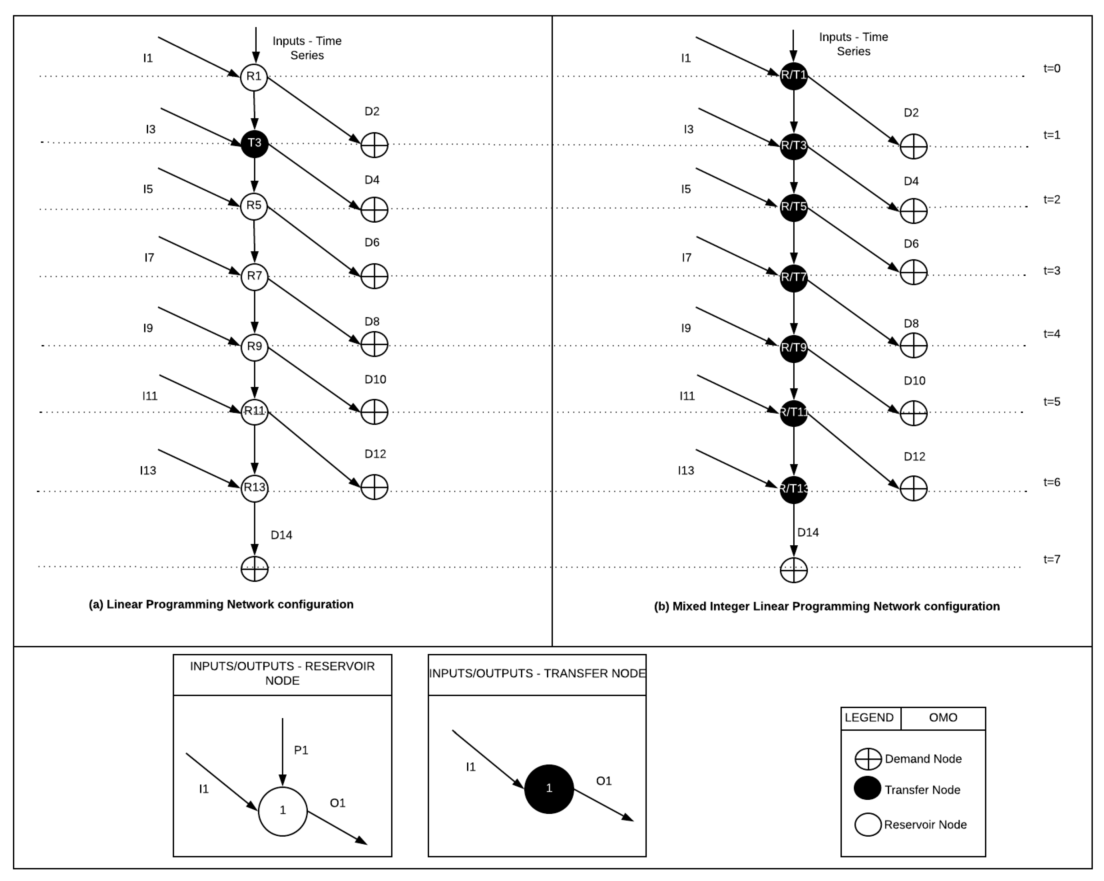
In general, as a first step the river system under study must be translated into a network configuration (Figure 1). There, 3 node types are distinguished: reservoir nodes (R), transfer nodes (T) and demand nodes (D) (Figure 2). A reservoir node represents the infrastructure to store water; a transfer node represents the downstream segment through which water flows; and a demand node represents the place where water is needed.

The magnitude of the flow through a network segment is encoded by the variable X. Different types of network segments are defined:

• X_i,n: input flow i (e.g., rivers, rainfall, runoff) reaching transfer node T_n;
• X_n,n+1: water flow between transfer node T_n and the consecutive transfer node T_n+1;
• X_n,r: water flow from transfer node T_n to reservoir node R_r;
• X_r,n: water flow from reservoir node R_r to transfer node T_n;
• X_n,d: water flow from transfer node T_n to demand node D_d.

Using these variables, all kinds of river segments can be defined and mimicked. In addition, the time that takes water to flow from one node to another has been identified as time step (t).

The specific, hypothetical network configuration studied in this paper is composed of 6 reservoir nodes, 1 transfer node and 7 demand nodes. Nodes are connected by segments that allow the transfer of water from one node to the next. The left panel (a) in Figure 1 is representing the network configuration of the LP model while the right panel (b) is representing the configuration of the MILP model. It is also noticeable that a transfer node is becoming a “candidate reservoirs” within the MILP network configuration.

3.2. Generic Optimisation Model

3.2.1. Linear Programming Model

The generic LP model [2 addresses a river system as a network configuration, described above, for optimizing the allocation of the water available in the nodes and segments to a set of spatially distributed water users of which the demand for water can vary in time. A complete description of this LP model can be found in [2]. However, a brief description of its main components is given in the following. The objective function consists of three terms. The first one pertains to the costs connected to the occurrence of floods along the river segments; in node n during the time step t. The second is related with the water demand (d) whereby not meeting the demand is associated with a penalty value. The third one expresses the penalties associated with the undercutting of the minimum allowed water volume in a reservoir (r).

$$\mathrm{minimize}{{\displaystyle \sum }}_{\mathrm{n}}{{\displaystyle \sum }}_{\mathrm{t}}\left({\mathrm{Q}}_{\mathrm{n}}\ast {\mathrm{T}}_{\mathrm{n},\mathrm{t}}^{+}\right)+{{\displaystyle \sum }}_{\mathrm{n}}{{\displaystyle \sum }}_{\mathrm{d}}{{\displaystyle \sum }}_{\mathrm{t}}\left({\mathrm{P}}_{\mathrm{n}}\ast {\mathrm{S}}_{\mathrm{n},\mathrm{d},\mathrm{t}}^{-}\right)+{{\displaystyle \sum }}_{\mathrm{r}}{{\displaystyle \sum }}_{\mathrm{t}}\left({\mathrm{U}}_{\mathrm{r}}\ast {\mathrm{SH}}_{\mathrm{r},\mathrm{t}}^{-}\right)$$

(1)

Furthermore, the LP model includes flow balance constraints in order to guarantee the balance between the inputs and outputs of water in a node considering water losses due to evaporation, infiltration, etc.) and the maximum and minimum capacity of reservoirs and river segments.

To ensure continuity of the water flow the LP model takes into account the maximal fraction of water that can leave a transfer node per time step, the minimal fraction of water that must be retained in the node per time step. As well as the water velocity causing a delay depending on the water speed.

3.2.2. Mixed Integer Linear Programming Model

For the MILP-model, transfer nodes (“candidate reservoirs”) are present in the network configuration (Figure 1b) are considered as potential locations for building a new reservoir with a predefined capacity (

Table 1. Characteristics of the ‘existing’ reservoirs included in the LP model.

Node	Initial Value [m3]	Minimum Capacity [m3]	Maximum Capacity [m3]
Reservoir 1 (R1)	15,000	10,000.00	300,000.00
Reservoir 5 (R5)	14,000	10,000.00	500,000.00
Reservoir 7 (R7)	15,000	10,000.00	450,000.00
Reservoir 9 (R9)	13,000	10,000.00	470,000.00
Reservoir 11 (R11)	16,000	10,000.00	350,000.00
Reservoir 13 (R13)	14,000	10,000.00	420,000.00

). The model is set up to determine those locations that keep the sum of costs related to not meeting demands, floods, water shortage in the reservoirs and the building and management the reservoirs to a minimum. Hence, the objective function of the previous LP model [2] must be extended with the building and management cost term (${\mathrm{BC}}_{\mathrm{n}}$) for every possible reservoir (${\mathrm{Y}}_{\mathrm{n}}$). ${\mathrm{Y}}_{\mathrm{n}}$ is a binary variable indicating whether location n has or has not been selected.

Objective function

$$\mathrm{minimize}{{\displaystyle \sum }}_{\mathrm{n}}{{\displaystyle \sum }}_{\mathrm{t}}\left({\mathrm{Q}}_{\mathrm{n}}\ast {\mathrm{T}}_{\mathrm{n},\mathrm{t}}^{+}\right)+{{\displaystyle \sum }}_{\mathrm{n}}{{\displaystyle \sum }}_{\mathrm{d}}{{\displaystyle \sum }}_{\mathrm{t}}\left({\mathrm{P}}_{\mathrm{n}}\ast {\mathrm{S}}_{\mathrm{n},\mathrm{d},\mathrm{t}}^{-}\right)+{{\displaystyle \sum }}_{\mathrm{n}}\left({\mathrm{BC}}_{\mathrm{n}}\ast {\mathrm{Y}}_{\mathrm{n}}\right)+{{\displaystyle \sum }}_{\mathrm{r}}{{\displaystyle \sum }}_{\mathrm{t}}\left({\mathrm{U}}_{\mathrm{r}}\ast {\mathrm{SH}}_{\mathrm{r},\mathrm{t}}^{-}\right)$$

(2)

In order to consider a candidate reservoir for selection, its characteristics such as maximum and minimum capacities must be taken into account (Table 1). This is done by updating the reservoir capacity constraints from the LP-model according to Equations (3)–(5). To specify the minimum number of the reservoirs allowed, Equation (6) has been added. No changes are required in the flow balance constraints, capacity constraints, limitation constraints, continuation constraints or time delay constraints as formulated for the LP-model [1,2].

Capacity constraints

Reservoir(s)

$${\mathrm{V}}_{\mathrm{r}}^{\mathrm{t}}-{\mathrm{OF}}_{\mathrm{r}}^{\mathrm{t}+}-{\mathrm{R}}_{\mathrm{r}\max }^{\mathrm{t}}={\mathrm{M}}_{\mathrm{r}}\ast \left(1-{\mathrm{Y}}_{\mathrm{r}}\right)$$

(3)

$$-{\mathrm{V}}_{\mathrm{r}}^{\mathrm{t}}\le -{\mathrm{R}}_{\mathrm{r}\min }^{\mathrm{t}}+\left({\mathrm{M}}_{\mathrm{r}}\ast \left(1-{\mathrm{Y}}_{\mathrm{r}}\right)\right)$$

(4)

$${\mathrm{OF}}_{\mathrm{r}}^{\mathrm{t}+}\le {\mathrm{M}}_{\mathrm{r}}\ast \left(1-{\mathrm{Y}}_{\mathrm{r}}\right)$$

(5)

Number of reservoirs

$${{\displaystyle \sum }}_{\mathrm{i}}{\mathrm{Y}}_{\mathrm{i}}^{}\ge 1$$

(6)

4. Results and Discussion

In order to verify both models (LP and MILP) and compare their outcome, the following assumptions have been defined for the network configurations of Figure 1a (LP) and Figure 1b (MILP): (a) Artificial time series of water inflow reflecting a biseasonal (dry-wet) year for three years (2014–2016) (Figure 3); (b) Loss function ($\propto$) is equal to 10%; (c) Time delays ($\mathsf{\delta }$) are equal to 10%; (d) Between 1% ($\mathsf{\gamma }$) and 20% ($\mathsf{\beta }$) of water must remain in a transfer node; (e) The time required to transfer water from one node to the next node is one day (24 h time step); (f) The maximum capacity of each river segment equals 8000 m³.

Table 1 shows the predefined characteristics of the 6 “existing” reservoirs. An initial value is given and also maximum and minimum capacity. All this values are hypothetical. While

Table 2. Water demand per node and penalty of not meeting demand in LP and MILP models.

Node	Demand [m3 per Time Step]	Penalty [euros per m3]
D2 (node 2)	200	2
D4 (node 4)	200	3
D6 (node 6)	200	2
D8 (node 8)	200	3
D10 (node 10)	200	2
D12 (node 12)	200	1
D14 (node 14)	200	3

clearly show is that all demand nodes have the same constant water demand of 200 m³ per day while the penalty for not meeting this demand is constant in time but variable between nodes.

4.1. Linear Programming Model

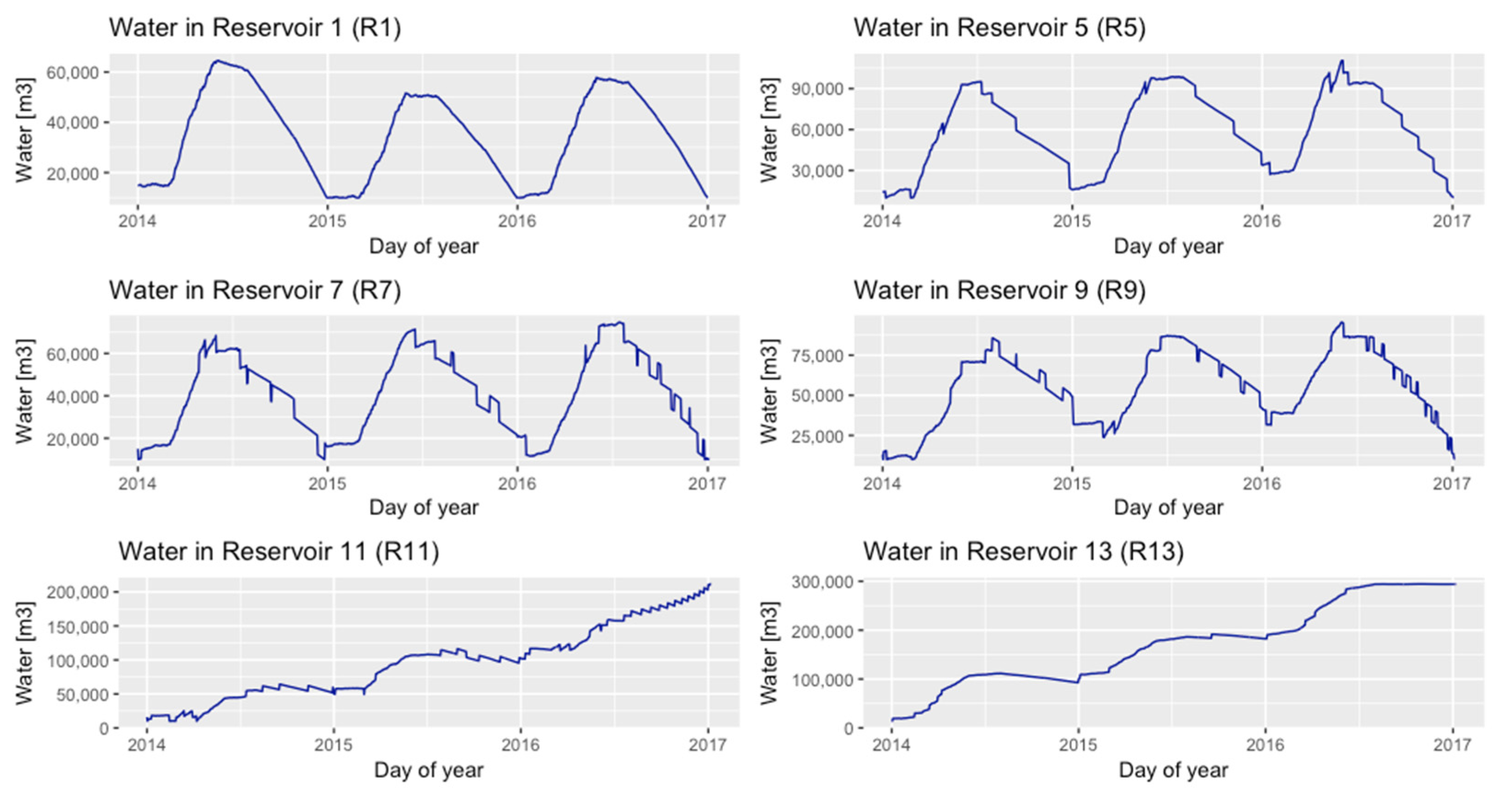
Figure 4 shows the fluctuation of the water volume present in each reservoir. The volume in reservoirs 1, 5, 7 and 9 fluctuates along with the dry and wet seasons. In contrast, reservoir 11 and 13 are constantly increasing their water levels. A slight decrease or steady-state is listed during the dry season. This filling-up process is occurring due to the limitation constraints (maximum and minimum capacities) introduced in the river segments. Besides, from Figure 4, it is noticeable the pattern of the filling-up and filling-down process is directly related with the inputs pattern.

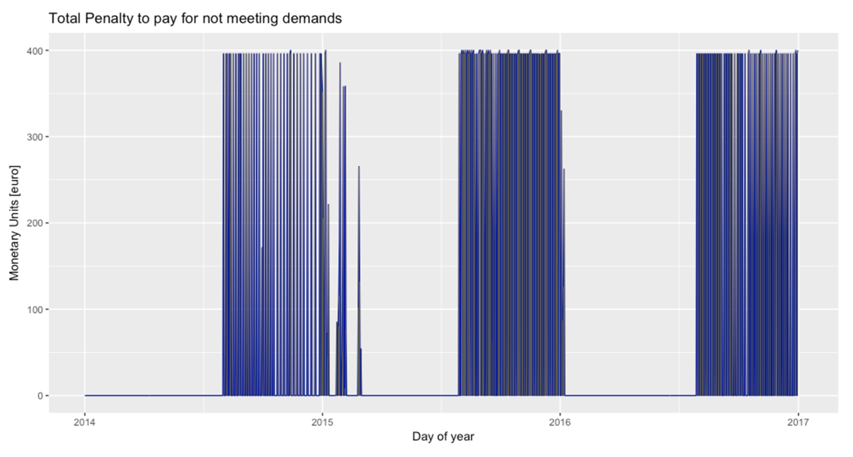
Figure 5 shows the penalty costs for the entire period (2014–2016). Penalties for not meeting the demands are applicable during the dry periods since in these periods, not enough water can be allocated to all nodes specially in 2, 4, 6, 8 and 10. Floods are avoided at all times so that no penalties apply. The summary of the total penalties is given in

Table 3. Penalty values for the LP-case.

Costs [euros]	Value [euros]
(a) Total penalty for not meeting demands	80,079.44
(b) Total penalty for flooding	0.00
(c) Total penalty for not reach the minimum in reervoirs	0.00
Total (a) + (b) + (c)	80,079.44

.

4.2. Mixed Integer Linear Programming Model

In this MILP-exercise, the main objective is to determine which of the node(s) (reservoir/transfer) must be turned into a reservoir given their predefined characteristics (i.e., location, initial water level, minimum and maximum capacity) in order to minimize the sum of penalties for not meeting demands, for occurrence of floods, for not respecting the minimally required water volume in the reservoirs and the building and management costs for the entire period. The data in Table 2 and

Table 4. Characteristics of the potential reservoirs considered in MILP model.

Node	Initial Value [m3]	Minimum Capacity [m3]	Maximum Capacity [m3]	Construction and Management Costs [euros]
Reservoir 1	0	10,000.00	300,000.00	500,000.00
Reservoir 3	0	10,000.00	400,000.00	450,000.00
Reservoir 5	0	10,000.00	500,000.00	550,000.00
Reservoir 7	0	10,000.00	450,000.00	430,000.00
Reservoir 9	0	10,000.00	470,000.00	510,000.00
Reservoir 11	0	10,000.00	350,000.00	470,000.00
Reservoir 13	0	10,000.00	420,000.00	490,000.00

, were used in this respect.

Figure 6 shows the water levels in the single selected reservoir (R11) throughout the entire period. The initialization value for each reservoir was set to 0 in order to model the initialization process (filling up) of the reservoir. In order to satisfy water demands, water coming from extra inputs were used as well as water from the reservoir. It is noticeable that the filling process is mainly occurring during the wet period (first half of each period). In this uses case some floods are present since the total sum of water necessary to satisfy demands exceed the maximum segment capacity (8000 m³).

Figure 5, includes a chart, related with the penalties for not meeting demands. In this case, the maximum penalty value is in the second half of the period coinciding with dry period. In this particular case, floods are occurring upstream the reservoir, this in order to meet all demands before the reservoir.

Table 5. Total values to pay as penalties and costs.

Costs [euros]	Value [euros]
(a) Total penalty to pay for not meeting demands	950,226.4
(b) Total penalty to pay for flooding	38.62
Total (a) + (b)	950,265.02
(c) Total Management costs	470,000.00
(d) Total penalty for not reach the minimum in reservoirs	0.00
Total value to pay (a) + (b) + (c) + (d)	1,420,265.02

, shows three types of payments associated with the model. (i) penalty costs for not meeting demands; (ii) penalty costs for flooding and (iii) costs related with management and building costs (per reservoir per the entire period). Besides, a chart of the first two components (i) and (ii) is shown in Figure 7.

5. Discussion

In order to compare the performance of the models, it is necessary to understand that the LP-model is using a configuration based on existing reservoirs with an initial water level different from zero while the MILP-model tries to draw the scenario where there are no fixed reservoirs only a set of “candidate” reservoirs with no water stored. Additionally, in the MILP models a management and construction cost is included to take into account the normal cost of building a new infrastructure, which is not the case in the LP-model. As future work, it is recommendable to associate a management cost to all existing reservoirs within the LP-model in order to create a more realistic use case. Besides, it is necessary to perform a sensitivity analysis to determine which of the parameters is the most sensitive. Moreover, the next step to undertake is to move this approach to a real study area use case.

6. Conclusions

By means of a hypothetical use case we show that a NFO-LP model, meant to optimally allocate river flow to demands which are distributed in space and variable in time, can be extended with binary variables that indicate the absence or presence of a reservoir of predefined capacity for a set of network nodes. The resulting MILP is capable of determining the single or multiple optimal reservoirs from a candidate reservoir set while simultaneously maximizing the demand satisfaction, minimizing excess water in the network segments and minimizing water shortage in the reservoirs. Provided that sufficient and sufficiently long time series of meteorological and/or discharge data are available, we believe that the MILP presents scope for strategic, reconnaissance and feasibility studies of dam projects in real world river systems characterized by seasonal flow dynamics and by competition among the water users.