Positively and Negatively Round Turbulent Buoyant Jets into Homogeneous Calm Ambient ^†

Abstract

A mathematical model has been employed to determine the characteristics of Boussinesq round buoyant jets which are injected horizontally or at an angle to horizontal, into a homogeneous, calm ambient. The solution of a system of three conservation first order nonlinear differential equations was obtained with a 4th Runge-Kutta scheme, using an entrainment coefficient which is related to the local Richardson number of the flow. Two types of positively and negatively buoyant jets were investigated (i) those where the buoyancy is a function of salinity henceforth called saline jets, and (ii) those where the buoyancy is a function of the temperature difference between jet and ambient fluid, henceforth called thermal jets.

1. Introduction

Round buoyant jets have been investigated over the past seven decades both, experimentally and numerically. There are only a few analytical solutions related mainly to vertical positively buoyant jets [1,2,3]. In numerical investigations the scientists use the entrainment equations of mass, momentum and buoyancy conservation which they integrate in one dimension, and compare the findings with earlier experiments. One of the issues for the integration of the entrainment equations is the appropriate selection of the entrainment coefficient to be used. Entrainment coefficients of vertical jets and plumes are quite different, therefore when used in a numerical algorithm they must be chosen properly. List in [4] has proposed two functions relating the entrainment coefficient in vertical buoyant jets to the local Richardson number. When the flow is jet-like (the momentum is dominant) the equations provide from jet growth asymptotically the jet entrainment coefficient, while when the buoyancy is dominant (plume-like flow) they provide the plume one. We must note that jet and plume entrainment coefficients used in the computations must be a priori defined.

Papanicolaou [1] has derived an analytical solution for vertical buoyant jets where the entrainment coefficient is a result of the solution that is based on the property of a constant buoyant jet expansion coefficient. In this paper a mathematical model has been developed to simulate the flow of round buoyant jets in a calm, uniform ambient fluid. The buoyant jets simulated are positively and negatively saline jets (buoyancy is a function of salinity difference between jet and ambient), or thermal jets (buoyancy is a function of temperature difference between jet and ambient. The results of the calculations were compared to existing (if available) experimental findings, in order to test the model’s validity. Furthermore, the model offers the opportunity to determine the flow characteristics along the buoyant jet trajectory, which could be quite difficult to obtain from experiments. The model can be used for research purposes as well as for engineering design. Companies which discharge treated liquid waste into an aquatic ambient can use this model in order to optimize the distribution system, as to minimize the negative impact of the treated liquid waste into the ambient. Also, researchers can use this model in the design of their experiment, e.g. to determine the dimensions of a dispersion tank.

2. Mathematical Model for Round Buoyant Jets

We consider a round vertical buoyant jet of density ρ_o out of a circular nozzle of diameter D with uniform exit velocity W, which discharges into a tank of finite volume filled with quiescent ambient fluid of uniform density ρ_a. The initial volume, specific (per unit mass) momentum and buoyancy fluxes are

Q_o = (πD²/4)W, and

(1)

M_o = Q_oW,

(2)

B_o = [(ρ_α − ρ_ο)/ρ_ο]gQ_o = g_ο0027 Q_o,

(3)

Following [4] we can define two length scales based upon the initial kinematic buoyant jet characteristics as $l_{\mathrm{Q}}={\mathrm{Q}}_{\mathrm{o}}/{\mathrm{M}}_{\mathrm{o}}^{1/2}$ and $l_{\mathrm{M}}={\mathrm{M}}_{\mathrm{o}}^{3/2}/{\mathrm{B}}_{\mathrm{o}}^{1/2}$, the ratio of which is the initial buoyant jet Richardson number ${\mathrm{R}}_{\mathrm{o}}={\mathrm{Q}}_{\mathrm{o}}{\mathrm{B}}_{\mathrm{o}}^{1/2}/{\mathrm{M}}_{\mathrm{o}}^{5/4}$.

The top-hat (uniform time-averaged velocity and density difference) equations of motion of round buoyant jets that discharge into calm ambient of uniform density according to Papakonstantis [5] are:

dq/ds = 2(πm)^1/2α,

(4)

dm/ds = (qβ/m)sinθ,

(5)

dθ/ds = (qβ/m²)cosθ,

(6)

dβ/ds = 0,

(7)

dx/ds = cosθ,

(8)

dz/ds = sinθ,

(9)

where s is the trajectory distance from the source, b, w and g’ the local jet width, average velocity and phenomenal gravity respectively, q = πb²w is the local volume flux, m = πb²w² and β = πb²wg’ are the local specific momentum and buoyancy fluxes respectively, x and y are the coordinates of s, θ is the local angle of the trajectory with respect to horizontal and α is the local entrainment coefficient. The local entrainment coefficient in a vertical buoyant jet is a function of [1]

Ri² = q²β/m^5/2

(10)

the local Richardson number squared, and it is written as

α = C_p{1 + Ri²/(2C_p)}/(2π^1/2),

(11)

where C_p = q/(m^1/2z) is the buoyant jet width parameter defined by [2] and evaluated from experiments by [6] to be a constant equal to 0.27. The initial buoyant jet parameters at the source are the volume flux Q_o, the specific momentum and buoyancy fluxes M_o and B_o respectively. The jet virtual origin where the computations start from is located at distance s_o from the source such as C_p = Q_o/(M_o^1/2s_o) that gives s_o = 3.28D when C_p = 0.27. Note that in negatively buoyant jets Ri² is negative and therefore the entrainment coefficient evaluated from Equation (11) may take negative values for large Ri, which has no physical meaning. Thus, when α < 0 in our computations we consider it to be equal to zero because otherwise the computed local volume flux is reduced, a process that thermodynamically speaking is contrary to the irreversible mixing process.

In saline jets the initial jet density is a function of the salinity and temperature. We assume that jet and ambient fluid temperatures are equal, therefore the initial buoyancy flux is conserved. The system of Equations (4)–(9) is solved with initial conditions s_o = 3.28D, q(s_o) = Q_o, m(s_o) = M_o, β(s_o) = Β_ο, θ(s_o) = θ_ο, x(s_o) = s_ocosθ_ο = X_o, and z(s_o) = s_osinθ_ο = Z_o.

In thermal jets the density is a function of the temperature difference between the jet and ambient fluid, therefore since the thermal expansion coefficient of water is variable, the jet specific buoyancy flux is variable (not conserved) with distance from the origin. The system of Equations (4)–(9) is solved with initial conditions s_o = 3.28D, q(s_o) = Q_o, m(s_o) = M_o, β(s_o) = Β_ο = {(ρ(T_a) − ρ(T_o))/ρ(T_o)}gQ_o, θ(s_o) = θ_ο, x(s_o) = s_ocosθ_ο = X_o, and z(s_o) = s_osinθ_ο = Z_o. In a thermal jet the heat flux is constant and we are using it to adjust the density difference between jet and ambient fluid as follows. The density of water as a function of temperature is

ρ = 999.9399 + 4.216485/10²Τ − 7.097451/10³Τ² + 3.509571/10⁵Τ³ − 9.9037785/10⁸Τ⁴

(12)

Using heat flux equation

q(T − Τ_α) = Q_o(T_o − T_α),

(13)

with q(s) known, we compute T(s) and from Equation (12) we compute the density ρ(s) so that the local buoyancy flux has changed to β(s) = {(ρ_a − ρ(s))/ρ(s)}gq(s) to be the new buoyancy flux for the next computational step.

The system of Equations (4)–(9) under initial conditions above was solved using a 4th order Runge-Kutta routine in Matlab^® environment.

3. Results

3.1. Positively Buoyant Saline Jets

In Figure 1 the results of our computations are presented and compared with earlier experiments [7] regarding the trajectory of round, positively buoyant saline jets that are discharged at different angles with respect to horizontal. Apparently our computations and measurements are found to be congruent. As far as the dilution is concerned in horizontal, round buoyant jets, the computed average dilution S = Δρ_ο/Δρ(s) normalized by the initial densimetric Froude number of the flow is plotted in Figure 2 versus z/l_M and compared to earlier experiments [8,9,10]. The average dilution computed by the model has been divided by a factor of 1.5 and converted to the mean dilution at the axis of the jet. It is evident that the model deviates from the measurements which we must note that are quite old.

3.2. Positively Buoyant Heated Jets (T_o > T_α)

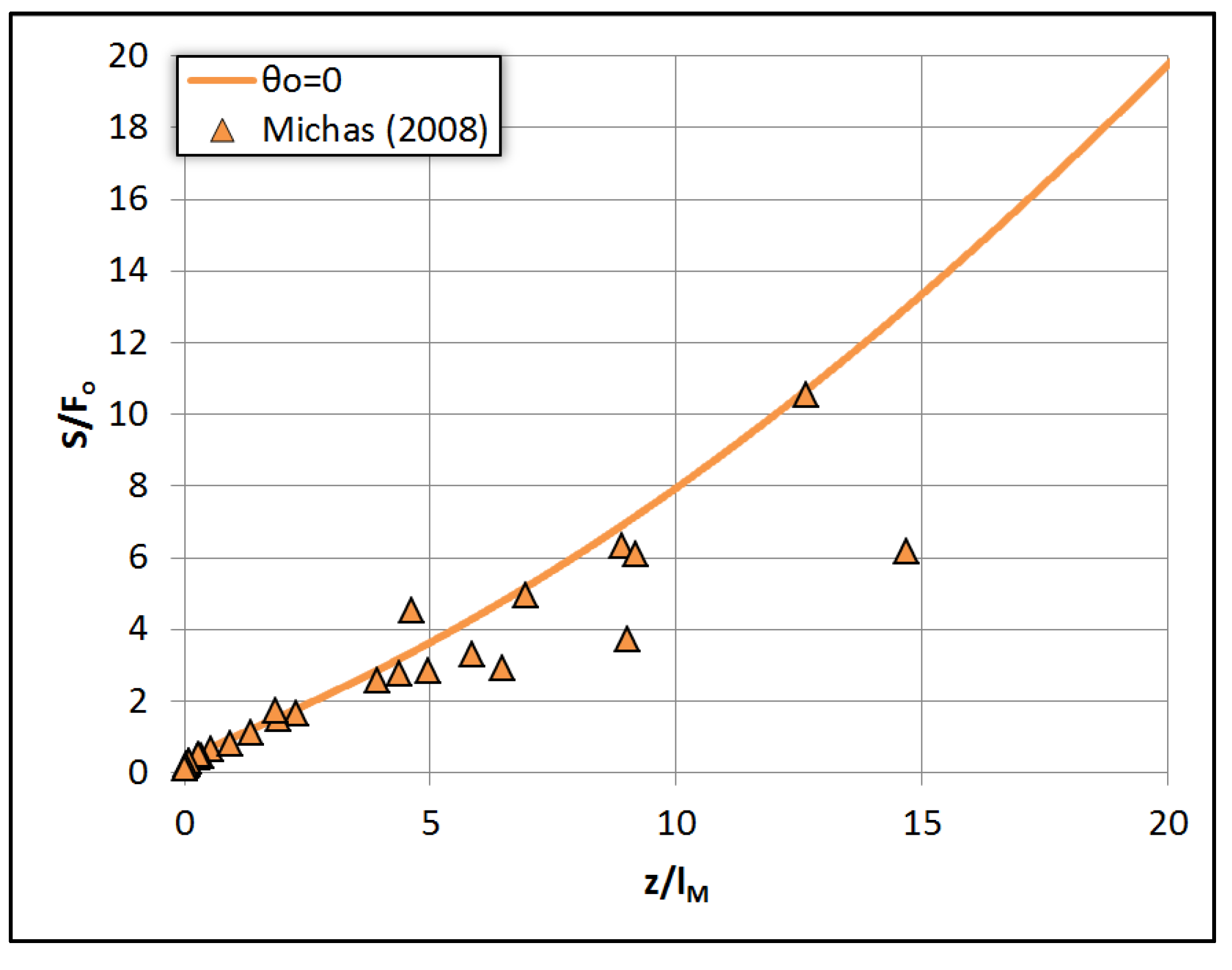
The normalized temperature difference between jet and ambient S = ΔΤ_ο/ΔΤ(s) divided by the initial Froude number (S/F_o) is plotted in Figure 3 against the normalized distance from the source s/l_M for positively buoyant (the jet being hotter than the ambient) heated jets. In Figure 4 experimental results [11] regarding the dilution of heated positively buoyant jets are compared to the results of the model. However, because the model calculates the average dilution and the experimental results are for the time-averaged dilution at the jet axis, the model results were divided by the value 1.4, so as to refer to the axis. It is evident that the model compares well with the experimental results.

3.3. Negatively Buoyant Saline Jets

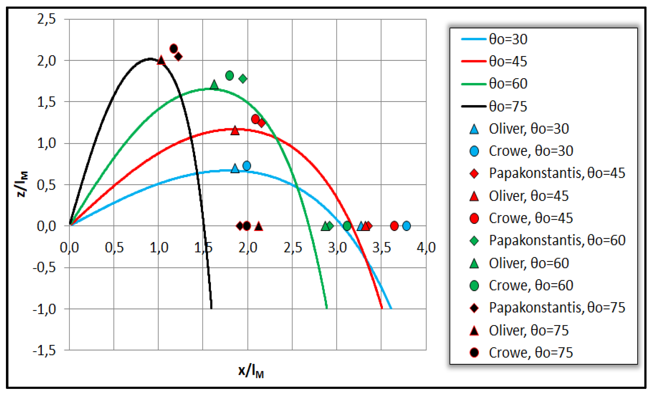
In Figure 5 the dimensionless trajectory of negatively buoyant saline jets is plotted with initial injection angles θ_o = 30–75°, initial Froude number F_o = 100 and density difference between jet and ambient Δρ = 25 kg/m³, and compared to experiments [5,12,13]. It is evident that the model results regarding the terminal trajectory height are near those measured by [5,12,13], while the return point horizontal distance of jet trajectory (at jet nozzle elevation) is underestimated.

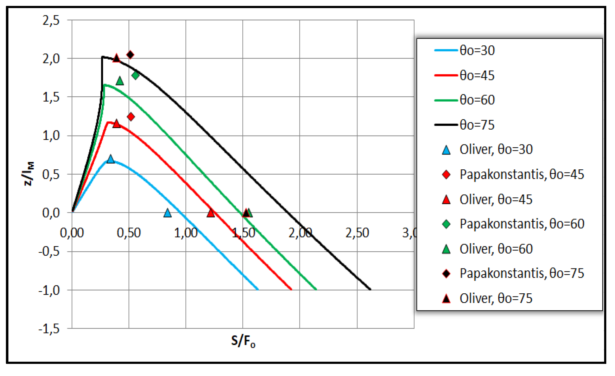
In Figure 6 the results from computations regarding the axial dilution of negatively saline jets are presented and compared to earlier experiments. The model obtains the average dilution, therefore the results are divided by the value 1.4, in order to convert the average dilution to mean dilution at the jet axis. It is evident that the model predictions regarding the axial dilution S_m and S_r at maximum elevation and return point respectively for injection angles θ_o = 30–60° compare well with Oliver’s data, while the axial dilution S_r deviates for θ_ο = 75°. Compared to Papakonstantis’ [5] measurements, our model predictions are on the lower side.

3.4. Negatively Buoyant Heated Jets (T_o > T_α)

The normalized trajectories of negatively buoyant heated jets with injection angles to horizontal θ_o = −30° to –75°, initial Froude number F_o = 100, and initial jet and ambient temperatures T_o = 30 °C and T_α = 20 °C respectively are plotted in Figure 7, where the experimental results of Vrachiolidis [14] regarding the maximum trajectory penetration depth and return distance are plotted for comparison. It is evident that the model compares well only with the results regarding injection angle θ_ο = 45°, while it overestimates all other parameters if compared to experiments. This may be due to the fact that [14] has used the shadowgraph method to determine the trajectory instead of measurements.

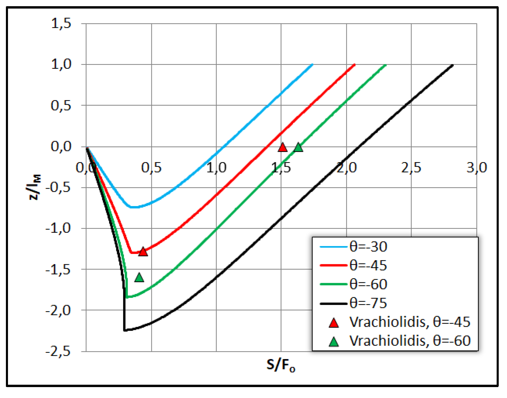
In Figure 8 the normalized dilution S/F_o has been plotted against the normalized elevation z/l_M along with centerline dilution measurements by [14]. The model obtains the average dilution and therefore the results have been divided by the value 1.4, to convert the average dilution to mean centerline dilution. It is obvious that the model predictions compare well with experiments regarding the axial dilution S_m and S_r at maximum elevation and return point of the trajectory respectively for angle θ_o = −45°, and the normalized dilution S_r for θ_ο = −60°.

3.5. Comparison of Positively Buoyant Saline, Hot and Cold Water Turbulent Jets

In the following paragraphs we are going to compare the results regarding jets which are positively buoyant and more specifically (i) fresh water jets into saline water pointing upwards, or saline jets in fresh water pointing downwards, (ii) hot water jets pointing upwards into cold water, and (iii) cold water jets into hotter water pointing downwards. The differences between the three types of jets are (a) saltwater jets maintain their initial buoyancy, (b) hot water jets in cold water have the initial buoyancy reduced with elevation and (c) cold water jets in hot water have the initial buoyancy increased with elevation, the last two being affected by the thermal expansion coefficient of water. In the figures that follow green color corresponds to parameters related to saline jets, red color corresponds to hot water jets injected into cold water and blue to cold water jets into hot water.

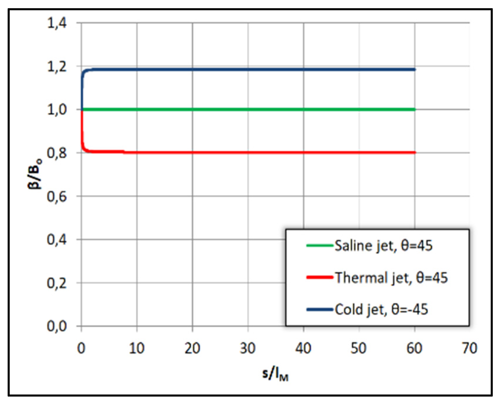
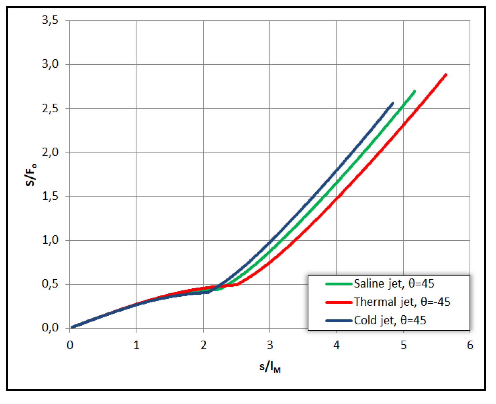
In Figure 9, Figure 10 and Figure 11 below we present the results from the computations of three positively buoyant jets in dimensionless form with the following initial characteristics (i) fresh water jet into saltwater with Δρ_ο = 25 kg/m³ at θ_ο = 45° and F_o = 100, (ii) hot water jet at T_o = 30 °C into cold ambient with temperature T_α = 20 °C, at θ_ο = 45° and F_o = 100, and (iii) cold water jet at T_o = 20 °C into hot water ambient with T_α = 30 °C, at θ_ο = −45° and F_o = 100. All three normalized trajectories are plotted upwards for comparison in Figure 9, where we observe that the saltwater trajectory stands in the middle of hot water one that goes further than the cold water trajectory. The same arrangement is evident in Figure 10 where the normalized dilution of the saline jet is greater than that of hot water jet into cold water but lower than that of cold water jet into hot water. In Figure 11 we have plotted the normalized local specific buoyancy flux β(s)/Β_ο versus the dimensionless distance s/l_M. It is evident that the heated jet buoyancy flux is reduced with distance from the origin, while it increases in the cold water jet and is constant in saline jets. The consequences are shown in Figure 9 and Figure 10 where we observe that cold water jets mix faster than saline jets which mix faster than the hot water ones.

3.6. Comparison of Negatively Buoyant Saline, Hot and Cold Water Turbulent Jets

In Figure 12, Figure 13 and Figure 14 below we present the results from the computations of three negatively buoyant jets in dimensionless form with the following initial characteristics (i) saltwater jet into fresh water with Δρ_ο = 25 kg/m³ at θ_ο = 45° and F_o = 100, (ii) hot water jet at T_o = 30 °C into cold ambient with temperature T_α = 20 °C, at θ_ο = −45° and F_o = 100, and (iii) cold water jet at T_o = 20 °C into hot water ambient with T_α = 30 °C, at θ_ο = 45° and F_o = 100. All three normalized trajectories are plotted upwards for comparison in Figure 12, where we observe that the saltwater trajectory stands in the middle of hot water one that goes higher than the cold water trajectory.

The same arrangement is evident in Figure 13 where the normalized dilution of the saline jet is greater than that of hot water jet into cold water but lower than that of cold water jet into hot water. In Figure 14 we have plotted the normalized local specific buoyancy flux β(s)/Β_ο versus the dimensionless distance s/l_M. Again, it is evident that the heated jet buoyancy flux is reduced with distance from the origin, while it increases in the cold water jet and is constant in saline jets. The consequences are shown in Figure 12 and Figure 13 where we observe that cold water jets mix faster than saline jets which mix faster than the hot water ones.

4. Conclusions

In the present paper which is based on the Diploma Thesis [15] of the first author, we have studied positively and negatively buoyant round turbulent jets in an unbounded homogeneous ambient fluid using a one-dimensional model based on conservation equations of mass, momentum and buoyancy fluxes. We have applied the set of conservation equations proposed by Papakonstantis [5], where we have made only one assumption, that the entrainment coefficient is a function of the local Richardson number of the flow [1], and it is always equal or greater than zero. The value of entrainment coefficient has not been predetermined as it is the usual practice in such flow modeling. The most important conclusions drawn from the previous sections are following.

In positively buoyant jets as the angle of inclination increases, the trajectory becomes shorter and approaches the vertical faster. The results from the calculations are congruent to earlier experiments regarding the trajectory [7] and mean (time-averaged) dilution along jet axis [8,9,10].

Cold water buoyant jets into hot water ambient have shorter trajectories and higher dilutions than saline jets, which have shorter trajectories and higher dilutions than hot water jets into cold ambient, regardless of the direction of buoyancy (positive or negative). This is probably due to the fact that the initial buoyancy of saline jets is conserved, while that of heated jets into cold water is reduced and that of cold water into hot water ambient increases, regardless of the direction of the flow. Therefore, one may conclude that increase in the specific buoyancy flux reduces the jet trajectory by increasing the dilution regardless of the flow direction.

The model predictions in negatively buoyant jets at an angle to horizontal are congruent to laboratory experiments regarding the maximum elevation of the trajectory, the horizontal distance from the nozzle where the maximum occurs and the average dilution there. They compare well with experiments regarding the return point of the trajectory at the elevation of injection and dilution for injection angles up to 60°, but they deviate from experiments for injection angle of 75° at the distance and average dilution. Regarding the heated negatively buoyant jets the model results compare well with experiments regarding the terminal height of the trajectory, the horizontal location of terminal height, the return point distance, as well as the axial dilution there.

References

- Papanicolaou, P.N. Analytical Solutions in Vertical Buoyant Jets. In Proceedings of the 11th HSTAM International Congress on Mechanics, Athens, Greece, 27-30 May 2016. [Google Scholar]
- List, E.J.; Imberger, J. Turbulent entrainment in buoyant jets and plumes. J. Hydraul. Div. 1973, 99, 1461–1474. [Google Scholar] [CrossRef]
- Yannopoulos, P.C. An improved integral model for plane and round turbulent buoyant jets. J. Fluid Mech. 2006, 547, 267–296. [Google Scholar] [CrossRef]
- Fischer, H.B.; List, E.J.; Koh, R.C.Y.; Imberger, J.; Brooks, N.H. Mixing in Inland and Coastal Waters; Academic Press. Elsevier: New York, NY, USA, 1979. [Google Scholar]
- Papakonstantis, I.G. Turbulent Round Negatively Buoyant Jets at an Angle in a Calm Homogeneous Ambient. Ph.D. Thesis, School of Civil Engineering, NTUA, Athens, Greece, 2009. (In Greek). [Google Scholar]
- Papanicolaou, P.N.; List, J.E. Investigations of round vertical turbulent buoyant jets. J. Fluid Mech. 1988, 195, 341–391. [Google Scholar] [CrossRef]
- Kikkert, G.A.; Davidson, M.J.; Nokes, R.I. Inclined negatively buoyant discharges. ASCE J. Hydraul. Eng. 2007, 133, 545–554. [Google Scholar] [CrossRef]
- Cederwall, K. The Initial Mixing on Jet Disposal into a Recipient. Chalmers University of Technology, Goteborg, Sweden, 1963. (In Swedish). [Google Scholar]
- Cederwall, K. Hydraulics of Marine Waste Water Disposal. Ph.D. Thesis, Hydraulic Division Rep. No. 42. Chalmers Institute of Technology, Göteborg, Sweden, 1968. [Google Scholar]
- Hansen, J.; Schroder, H. Horizontal Jet Dilution Studies by Use of Radioactive Isotopes; Acta Polytechnica Scandinavia, Civil Engineering and Building Construction Series 49; Danish Academy of Technical Sciences: Copenhagen, Denmark, 1968. [Google Scholar]
- Michas, S.N. Experimental Investigation of Horizontal Round and Non-Axisymmetric Buoyant Jets in a Uniform Calm Ambient. Ph.D. Thesis, Hydromechanics and Environmental Engineering Laboratory, Department of Civil Engineering, University of Thessaly, Filellinon, Volos, Greece, 2008. (In Greek). [Google Scholar]
- Oliver, C.J. Near Field Mixing of Negatively Buoyant Jets. Ph.D. Thesis, University of Canterbury, Christchurch, New Zealand, 2012. [Google Scholar]
- Crowe, A.T. Inclined Negatively Buoyant Jets and Boundary Interaction. Ph.D. Thesis, University of Canterbury, Christchurch, New Zealand, 2013. [Google Scholar]
- Vrachiolidis, A. Negatively Buoyant Heated Turbulent Jets at an Angle. Diploma Thesis, School of Civil Engineering, National Technical University of Athens, Greece, 2016. (In Greek). [Google Scholar]
- Fragkou, A. Turbulent Round Positively and Negatively Buoyant Jets in a Homogeneous Calm Ambient. Diploma Thesis, School of Civil Engineering, National Technical University of Athens, Greece, 2017. (In Greek). [Google Scholar]
Figure 1.
Comparison between model and experimental results regarding the trajectory of positively buoyant saline jets.
Figure 2.
Comparison between model and experimental results regarding the axial dilution S/Fo of positively buoyant saline jets.
Figure 3.
Dimensionless average dilution S/Fo as a function of s/lM of positively buoyant heated jets for θο = 45°, Fo = 100, To = 20–60 °C, Τα = 10–20 °C.
Figure 4.
Comparison between model and experimental results [11] regarding the axial dilution S/Fo of positively buoyant heated jets.
Figure 5.
Comparison between model and experimental results regarding the trajectory of negatively buoyant saline jets.
Figure 6.
Comparison between model predictions and experiments regarding the axial dilution at the terminal height Sm/Fo and return point Sr/Fo of negatively buoyant saline jets.
Figure 7.
Comparison between model and experiments [14] regarding the normalized trajectory of negatively buoyant heated jets.
Figure 8.
Comparison between model and experiments regarding the axial dilution Sm/Fo at terminal height and Sr/Fo at the return point of negatively buoyant heated jets.
Figure 9.
Normalized positively buoyant jet trajectory at θο = 45°.
Figure 10.
Normalized positively buoyant jet dilution S/Fo at θο = 45°.
Figure 11.
Normalized buoyancy flux β/Βο of positively buoyant jet at θο = 45°.
Figure 12.
Comparison between negatively buoyant jets regarding their trajectory.
Figure 13.
Comparison between negatively buoyant jets regarding their average dilution S/Fo.
Figure 14.
Comparison between negatively buoyant jets regarding their buoyant power β/Βο.
Publisher’s Note: MDPI stays neutral with regard to jurisdictional claims in published maps and institutional affiliations. |
© 2018 by the authors. Licensee MDPI, Basel, Switzerland. This article is an open access article distributed under the terms and conditions of the Creative Commons Attribution (CC BY) license (https://creativecommons.org/licenses/by/4.0/).
Share and Cite
MDPI and ACS Style
Fragkou, A.; Papanicolaou, P. Positively and Negatively Round Turbulent Buoyant Jets into Homogeneous Calm Ambient. Proceedings 2018, 2, 572. https://doi.org/10.3390/proceedings2110572
AMA Style
Fragkou A, Papanicolaou P. Positively and Negatively Round Turbulent Buoyant Jets into Homogeneous Calm Ambient. Proceedings. 2018; 2(11):572. https://doi.org/10.3390/proceedings2110572
Chicago/Turabian StyleFragkou, Anastasia, and Panos Papanicolaou. 2018. "Positively and Negatively Round Turbulent Buoyant Jets into Homogeneous Calm Ambient" Proceedings 2, no. 11: 572. https://doi.org/10.3390/proceedings2110572