Adaptive Neural Control for a Class of Random Fractional-Order Multi-Agent Systems with Markov Jump Parameters and Full State Constraints

Abstract

Based on an adaptive neural control scheme, this paper investigates the consensus problem of random Markov jump multi-agent systems with full state constraints. Each agent is described by the fractional-order random nonlinear uncertain system driven by random differential equations, where the random noise is the second-order stationary stochastic process. First, in order to deal with the unknown functions with Markov jump parameters, a radial basis function neural network (RBFNN) structure is introduced to achieve approximation. Second, for the purpose of keeping the agents’ states from violating the constraint boundary, the tan-type barrier Lyapunov function is employed. By using the stochastic stability theory and adopting the backstepping technique, a novel adaptive neural control design method is presented. Furthermore, to cope with the differential explosion problem in the design course, the extended state observer (ESO) is developed instead of neural network (NN) approximation or command filtering techniques. Finally, the exponentially noise-to-state stability in the mean square is analyzed rigorously by the Lyapunov method, which guarantees the consensus of the considered multi-agent systems and all the agents’ outputs are bounded in probability. Two simulation examples are provided to verify the effectiveness of the suggested control strategy.

1. Introduction

Over the past two decades, collaborative control of multi-agent systems (MASs) has received increasing attention due to its wide range of applications in the fields of unmanned aerial vehicle formation, intelligent robotics, and sensor networks [1,2,3]. MASs are collections of multiple agents, the essence of which is to transform large and complex systems into easily manageable systems that communicate and coordinate with each other [4]. Particularly, as a fundamental research area in collaborative control, the consensus problem focuses on investigating whether agents with different initial states can achieve an agreement under the designed control protocols [5,6]. Existing research on the multi-agent consensus problem is distributed across various system models, where each agent system can be described by first- [7,8], second- [9,10], high-order dynamics [11,12] or a fractional-order dynamics model [13]. It is worth noting that the study of fractional-order multi-agent systems (FOMASs) have recently received increasing attention due to their ability to accurately describe the dynamical properties of physical systems.

For the actual applications, it is worth considering that practical engineering systems are subject to sudden environmental changes and random changes in structure or parameters during operation. Due to the ability to effectively model these complex situations, Markov jump systems [14] have stimulated research interest among scholars and yielded many useful results. Ref. [15] discussed the stochastic stability of linear Markov jump systems with time delay. Ref. [16] studied feedback control of continuous-time linear Markov jump systems with singular regimes. Up to now, it is clear that most existing studies of Markov jump systems tend to use stochastic differential equations (SDEs) with white noise [17,18]. However, dynamical models based on SDEs driven by Wiener processes are not applicable to many practical situations. It is pointed out in [19,20] that Wiener processes are non-differential almost everywhere, and ideal white noise with infinite bandwidth cannot occur in the real world. Therefore, it is reasonable to describe Markov jump systems by random differential equations (RDEs), which contain second-order moment random noises [21,22]. Utilizing the improved backstepping method, an adaptive tracking controller is proposed for the random pure-feedback nonlinear Markov switching systems in [21]. A backstepping controller is developed to deal with the tracking control problem for the random nonlinear Markov switching systems in [22].

Furthermore, due to the good nonlinear approximation ability, the NN technique and fuzzy logic systems (FLSs) are becoming more widely used, respectively [23,24,25]. Combined with the backstepping approach, many adaptive control strategies have been applied to Markov jump nonlinear systems. For example, in [26], an adaptive fuzzy tracking controller is designed for a class of strict feedback Markov jump systems with multi-source uncertainty. In [27], a neural network-based adaptive controller is designed for high-order nonlinear stochastic switching systems containing Markov jump parameters. In [28], a fractional power-based adaptive command filtering backstepping algorithm is designed, taking into account the Markov jump structure. Note that the relevant results obtained apply only to the single systems with Markov jump parameters. Particularly, with regard to Markov jump MASs, various control strategies have been proposed to deal with the consensus problem of Markov jump MASs, such as event-triggered control [29,30], output feedback control [31], and robust control [32]. For high-order nonlinear Markov jump MASs, how to achieve target control through the adaptive neural control method needs to be further explored. In addition, how to address the differential explosion problem that obtains during the backstepping design of high-order systems while ensuring the stability of the system is also a challenge research area. In [33], NNs are used to globally approximate the nonlinear functions and the derivatives of the virtual control laws. In [34], the command filter is introduced into the control system to obtain the derivatives of the virtual control function. However, as an easier computational and parametric estimation method, devising the ESO to deal with the differential explosion problem is potentially promising.

All of the above studies are based on integer-order Markov jump MASs; actually, the adaptive control methods are also often applied to fractional-order systems to achieve a wide range of control objectives [34,35,36]. Introducing fractional-order Markov jump MASs and then developing an adaptive strategy for such systems has remained unaddressed so far. Moreover, in engineering practice, constraints on the system state are necessary to avoid a wide range of vibrations and to obtain smooth control performance. The barrier Lyapunov function (BLF) [37] is usually constructed and widely used to keep the state variables within constraints. The common BLFs, such as log-type BLF [38] and integral-type BLF [39], always fail in the case of infinite constraint requirements. To solve this problem, tan-type BLF (TBLF) is proposed [40]. Regardless of whether the state has constraint requirements or not, the system still works properly. So how to design the tracking controller for fractional-order Markov jump MASs with state constraints is meaningful.

Based on previous analysis, this paper aims to investigating the consensus tracking problem of FOMASs with Markov jump parameters. Considering the disturbances of Markov jump factors, the adaptive RBFNN and ESO estimation methods are finally integrated in the context of the backstepping technique. An adaptive neural controller based on TBLF is designed to ensure that all signals in the closed-loop system are bounded under Markov jump signals and that state constraints are not violated. Compared with previous research, the main contributions of this paper are as follows.

(1)

In contrast to the consensus studies for MASs [41,42], to enhance the system performance, we take a novel fractional-order state-constrained multi-agent system with Markov jump parameters driven by random differential equations into account, in which the random noise is the second-order stationary stochastic process.

(2)

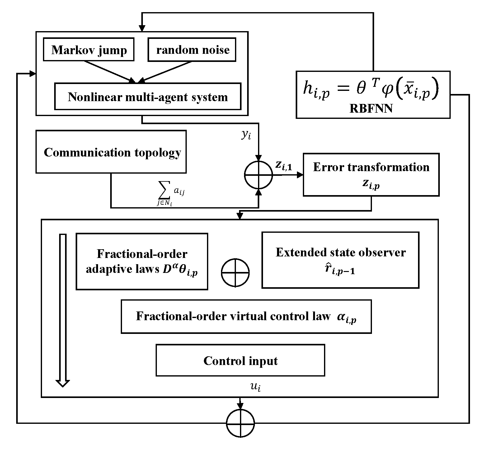
Unlike [27], for a class of state-constrained FOMASs with Markov jump structures, this paper proposes the approximation tracking method of adaptive neural control, combining NNs and the backstepping technique together to achieve the consensus control target and ensure the system’s noise-to-state stability.

(3)

Different from [33,34], in which the NN technique and the command filtering method are adopted to handle the derivatives of the virtual control laws, respectively, in this paper, to cope with the differential explosion problem in the design course, the ESO estimation method is developed.

The remainder of this study is constructed as follows. Section 2 gives the preliminaries and formulation of this paper, such as the basic theory of fractional multi-agent and Markov jump systems. In Section 3, an adaptive backstepping control scheme and the stability analysis are presented. In Section 4, the obtained theoretical results are verified by two examples. Section 5 gives the conclusions. The abbreviations used in this article are summarized in the Abbreviations.

2. Problem Formulation and Preliminaries

2.1. Fractional Calculus

The Caputo fractional derivative [43] is defined as

$$\begin{array}{c}\hfill {}_0{}^{C}D_t^{\alpha }f\left(t\right)=\frac{1}{\Gamma \left(\nu -\alpha \right)}{\int }_0^t\frac{f^{\left(\nu \right)}\left(\tau \right)}{{\left(t-\tau \right)}^{1+\alpha -\nu }}d\tau \end{array}$$

(1)

where $\nu \in N$ and $\nu -1<\alpha \le \nu$, $\Gamma \left(z\right)={\int }_0^{\infty }{t}^{z-1}{e}^{-t}dt$ is the Gamma function. In this paper, we examine the fractional order within the range of [0, 1].

Lemma 1 

([44]). For real numbers $\alpha ,v$ and κ satisfying $\alpha \in \left(0,1\right)$

$$\begin{array}{c}\hfill \frac{\pi \alpha }{2}<v<min\left\{\pi ,\pi \alpha \right\}\end{array}$$

(2)

and for all integers $\nu \ge 1$, we obtain

$$\begin{array}{c}\hfill E_{\alpha ,\kappa }\left(\varsigma \right)=-\sum _{j=1}^{\infty }\frac{1}{\Gamma \left(\kappa -\alpha j\right)}+o\left(\frac{1}{{\left|\varsigma \right|}^{\nu +1}}\right)\end{array}$$

(3)

when $\left|\varsigma \right|\to \infty ,v\le \left|arg\left(\varsigma \right)\right|\le \pi$.

Lemma 2 

([44]). If v satisfies the condition of Lemma 1, the inequality relation holds:

$$\begin{array}{c}\hfill \left|E_{\alpha ,\kappa }\left(\varsigma \right)\right|\le \frac{\mu }{1+\left|\varsigma \right|}\end{array}$$

(4)

where $\alpha \in \left(0,2\right)$ and κ is an arbitrary real number, $\mu >0$, $\upsilon \le \left|arg\left(\varsigma \right)\right|\le \pi$, and $\left|\varsigma \right|\ge 0$.

2.2. Graph Theory

This paper employes a connected undirected $W=\left(v,\delta ,\overline{A}\right)$ where $v=\left\{n_1,\dots ,n_N\right\}$ and $\overline{A}=\left\{a_{ij}\right\}\in {\mathbb{R}}^{N\times N}$ is the adjacency matrix. For agent i, define the edge set as $\delta =\left\{\left(n_i,n_j\right)\right\}\in v\times v$ and the neighbor set as $N_i=\left\{j\left|\left(n_i,n_j\right)\in \delta \right.\right\}$.

For matrix $\overline{A}=\left\{a_{ij}\right\}$, $a_{ij}$ is represented as if $\left(n_i,n_j\right)\notin \delta$, $a_{ij}=0$; otherwise, $a_{ij}\ne 0$, and it is supposed that $a_{ii}=0$. We utilize $Q=diag\left(q_1,\dots ,q_N\right)$ as the diagonal matrix where $q_i={\sum }_{j\in n=N_i}{a}_{ij}$ and define the Laplacian matrix as $L=\left[l_{ij}\right]=Q-\overline{A}\in {\mathbb{R}}^{N\times N}$, in which $l_{ii}={\sum }_{j=1}^N{a}_{ij}$ and $l_{ij}=-a_{ij}$ for $i\ne j$.

2.3. Random Nonlinear Markov Jump Multi-Agent System

The random nonlinear FOMASs with Markov jump parameters is considered as follows:

$$\begin{array}{c}\hfill \left\{\begin{array}{c}{D}^{\alpha }{x}_{i,1}=x_{i,2}+h_{i,1}({\overline{x}}_{i,1},t,r\left(t\right))+g_{i,1}({\overline{x}}_{i,1},t,r\left(t\right)){\xi }_{i,1}\left(t\right)\hfill \\ D^{\alpha }{x}_{i,p}=x_{i,p+1}+h_{i,p}({\overline{x}}_{i,p},t,r\left(t\right))+g_{i,p}({\overline{x}}_{i,p},t,r\left(t\right)){\xi }_{i,p}\left(t\right),p=2,\cdots ,n-1\hfill \\ D^{\alpha }{x}_{i,n}=u_i+h_{i,n}({\overline{x}}_{i,n},t,r\left(t\right))+g_{i,n}({\overline{x}}_{i,n},t,r\left(t\right)){\xi }_{i,n}\left(t\right)\hfill \\ y_i=x_{i,1}\hfill \end{array}\right.\end{array}$$

(5)

in which $y_i$ is the system output and $h_{i,p}\left(·\right)$ are unknown nonlinear functions. $u_i$ represents the control input. Design the system state vectors ${\overline{x}}_{i,p}={(x_{i,1},\cdots ,x_{i,p})}^T\in {\mathbb{R}}^p$. The stochastic process $\xi \left(t\right)$ is defined on the complete probability space $\left(\Omega ,{\mathcal{F}}_t,\mathrm{P}\right)$, where ${\mathcal{F}}_t\left(t\ge t_0\right)$ satisfies the usual conditions. $r\left(t\right)$ is a right continuous homogeneous irreducible Markov process with values in a finite mode space $S=\left\{1,2,\dots ,M\right\}$ and the matrix $P={\left(p_{km}\right)}_{M\times M}$.

$$P_{km}\left(\Delta \right)=P_{km}\left\{r(t+\Delta )=m\left|r\right(t)=k\right\}=\left\{\begin{array}{c}{p}_{km}\Delta +o\left(\Delta \right),k\ne m\hfill \\ 1+p_{kk}\Delta +o\left(\Delta \right),k=m\hfill \end{array}\right.$$

(6)

where $p_{kk}=-{\sum }_{m=1,m\ne k}^M{p}_{km}$, $p_{km}\ge 0$ denotes the transition rate from k to m.

Definition 1. 

For $V\left(x\left(t\right),r\left(t\right)\right)\in C\left({\mathbb{R}}_{+}\times \mathbb{R}\times S;{\mathbb{R}}_{+}\right)$, similar to [45], we introduce the infinitesimal generator by

$$\mathcal{L}V\left(x,t,k\right)=V_t\left(x,t,k\right)+V_x\left(x,t,k\right)\dot{x}\left(t\right)+\Pi V$$

(7)

where $V_t\left(x,t,k\right)=\frac{\partial V}{\partial t}$, $V_x\left(x,t,k\right)=\frac{\partial V}{\partial x}$, $\Pi V={\displaystyle \sum _{m=1}^M}{q}_{km}V\left(x,t,m\right),k\in S$.

According to Definition 1, considering that the FOMAS is designed in this paper, we present

$$\mathcal{L}V\left(x,t,k\right)=D_t^{\alpha }V\left(x,t,k\right)+V_x\left(x,t,k\right)D^{\alpha }x\left(t\right)+\Pi V.$$

(8)

Assumption 1. 

Due to continuous and ${\mathcal{F}}_t-$ adapted characteristics of the random process ${\xi }_t$ composed of the second-order moment, a positive constant K satisfies ${sup}_{t\ge t_0}\mathrm{E}{\left|\xi \left(t\right)\right|}^2\le K$.

Assumption 2 

([36]). In control engineering, the RBFNN technique is utilized to compensate for the unknown nonlinearities in MASs. Specifically, the unknown nonlinear functions $h_{i,p}\left({\overline{x}}_{i,p}\right)$ can be expressed as

$$h_{i,p}\left({\overline{x}}_{i,p}|{\theta }_{i,p}\right)={\theta }_{i,p}^T{\phi }_{i,p}\left({\overline{x}}_{i,p}\right),1\le p\le n$$

(9)

in which ${\phi }_{i,p}\left({\overline{x}}_{i,p}\right)$ delegates Gaussian basis function vector, and ${\theta }_{i,p}$ represent the vectors of the unknown ideal constant. Given a continuous unknown function $h\left(x\right)$ defined on the compact set ${\Omega }_x$, there exist the neural networks ${{\theta }^{*}}^T\phi \left(x\right)$ and the arbitrary accuracy $\epsilon \left(x\right)$ satisfying $h\left(x\right)={{\theta }^{*}}^T\phi \left(x\right)+\epsilon \left(x\right)$, where ${\theta }^{*}$ is the ideal weight vector defined by ${\theta }^{*}=arg{min}_{\theta \in {\Omega }_{\theta }}$$\left[{sup}_{x\in {\Omega }_x}\left|h\left(x\right)-{\theta }^T\phi \left(x\right)\right|\right]$, and the parameter estimation error is ${\tilde{\theta }}_{i,p}={\theta }_{i,p}^{*}-{\theta }_{i,p}$. $\epsilon \left(x\right)$ denotes the minimum approximation error. There exists a positive constant ${\epsilon }_0$, such that $\epsilon \left(x\right)\le {\epsilon }_0$, ${\epsilon }_0>0$.

Lemma 3 

([22]). For any mode k, there exists a positive continuously differentiable function $V\left(x,t,k\right)$ satisfying

$$\mathcal{L}V\left(x,t,k\right)\le -\gamma \left(\left|x\right(t\left)\right|\right)+c|\xi \left(t\right){|}^2$$

(10)

$${\gamma }_1\left(\left|x\left(t\right)\right|\right)\le V\left(x\left(t\right),k\right)\le {\gamma }_2\left(\left|x\left(t\right)\right|\right)$$

(11)

$$\frac{\partial V\left(x\left(t\right)\right)}{\partial x}{h}_p\left(x\left(t\right),t\right)+d{\left|\frac{\partial V\left(x\left(t\right)\right)}{\partial x}{g}_p\left(x\left(t\right),t\right)\right|}^2\le -\gamma \left(\left|x\left(t\right)\right|\right)$$

(12)

where ${\gamma }_1$ and ${\gamma }_2$ are functions of class ${\kappa }_{\infty }$, and c is a positive constant. A unique global solution exists in system (5). If $\gamma \left({\gamma }_2^{-1}(·)\right)$ is convex, then system (5) demonstrates noise-to-state stability in probability. Additionally, the state of system (5) exhibits an asymptotic gain in probability, implying an ultimate bound for the state in probability.

Lemma 4 

([22]). Under Assumption 1, if there exists a positive function $V\left(t,x,r\right)$, constants D and $c_0>0$, such that for $\forall t\ge t_0$,

$$\begin{array}{cc}\hfill & \underset{n\to \infty }{lim}infV\left(t,x,r\right)=\infty \hfill \\ & EV\left(t\wedge {\lambda }_n,x\left(t\wedge {\lambda }_n\right),r\left(t\wedge {\lambda }_n\right)\right)\le D{e}^{c_{0}t}\hfill \end{array}$$

(13)

Thus, system (5) possesses a unique solution $x\left(t\right)$ when $t\ge t_0$.

Lemma 5 

([46]). For any $\theta ,\vartheta \in {\mathbb{R}}^n$, one obtains

$${\theta }^T\vartheta \le \frac{{\omega }^r}{r}{\left|\theta \right|}^r+\frac{1}{\upsilon {\omega }^{\upsilon }}{\left|\vartheta \right|}^{\upsilon }$$

(14)

where $r>1$, $\upsilon >1$, $\omega >0$, and $\left(\upsilon -1\right)\left(r-1\right)=1$.

2.4. Tan-Type BLFs

Lemma 6 

([47]). To deal with performance constraints, the TBLF of the ith agent is considered as follows:

$$V_{i,m}=\frac{k_{i,bm}^2}{\pi }tan\left(\frac{\pi z_{i,m}^2}{2k_{i,bm}^2}\right)$$

(15)

where $i=1,\dots ,N$, $m=1,\dots ,n$. By using L’Hospital rule, we have

$$\underset{k_{i,bm}\to \infty }{lim}\frac{k_{i,bm}^2}{\pi }tan\left(\frac{\pi z_{i,m}^2}{2k_{i,bm}^2}\right)=\frac{z_{i,m}^2}{2}.$$

(16)

Therefore, the proposed TBLF will be turned into the conventional Lyapunov function and the design method is also effective for systems without constraints.

3. Main Results

Theorem 1. 

For the Markov jump FOMASs (5) where Assumptions 1–2 hold, designing the virtual control laws (29), (42), (53), and combining the adaptive laws (30), (31), (43), (54), (63) and control input (62) together, signals $x_{i,1}$ converge to the consensus of considered nonlinear FOMASs asymptotically. It can be verified that the tracking error of the closed-loop system in the mean-square sense can be converged to a zero neighborhood that is arbitrarily small without violating the constraints we set.

Proof. 

Specify the error variables in the following manner:

$$\begin{array}{cc}\hfill & z_{i,1}=\sum _{j\in N_i}{a}_{ij}\left(y_i-y_j\right)+b_i(y_i-y_d)\hfill \\ & z_{i,p}=x_{i,p}-{\alpha }_{i,p-1},p=2,\cdots ,n\hfill \end{array}$$

(17)

where $s_{i,p}$ represents the tracking error, and ${\alpha }_{i,p-1}$ is the virtual controller.

Step 1. First, let $z_1={[z_{1,1}\cdots z_{N,1}]}^T$, $\overline{y}={[y_1\cdots y_N]}^T$, $\mathcal{A}=diag\left\{b_i\right\}$, $H=\mathcal{A}+L$,

$$s_1=\overline{y}-y_d$$

(18)

$$z_1=H{s}_1$$

(19)

where $s_1={[s_{1,1}\cdots s_{N,1}]}^T$. Referring to Lemma 6, construct the first Lyapunov function:

$$\begin{array}{cc}\hfill V_1=& \sum _{i=1}^N\left(\frac{k_{i,b1}^2}{\pi }tan\left(\frac{\pi z_{i,1}^2}{2k_{i,b1}^2}\right)+\frac{1}{2{\sigma }_{i,1}}{\tilde{\theta }}_{i,1}^T{\tilde{\theta }}_{i,1}+\sum _{j\in N_i}\frac{a_{ij}}{2{\sigma }_{j,1}}{\tilde{\theta }}_{j,1}^T{\tilde{\theta }}_{j,1}\right)\hfill \end{array}$$

(20)

where $k_{i,b1}$, ${\sigma }_{i,1}$ and ${\sigma }_{j,1}$ are the parameters we set. Define ${\displaystyle \sum _{j\in N_i}}{a}_{ij}=d_i$, according to the system (5), and we have

$$\begin{array}{cc}\hfill D^{\alpha }{z}_{i,1}=& \left(b_i+\sum _{j\in N_i}{a}_{ij}\right){D^{\alpha }y}_i-\sum _{j\in N_i}{a}_{ij}{D^{\alpha }y}_j-b_i{D^{\alpha }y}_r\hfill \\ \hfill =& \left(b_i+d_i\right)\left({\alpha }_{i,1}+z_{i,2}+h_{i,1}+g_{i,1}{\xi }_{i,1}\right)-\sum _{j\in N_i}{a}_{ij}\left(x_{j,2}+h_{j,1}+g_{j,1}{\xi }_{j,1}\right)-b_i{D^{\alpha }y}_r.\hfill \end{array}$$

(21)

To simplify the equation, we set ${\varpi }_{i,1}=\frac{z_{i,1}}{{cos}^2\left(\frac{\pi z_{i,1}^2}{2k_{i,b1}^2}\right)}$, and then we can obtain

$$\begin{array}{cc}\hfill \mathcal{L}{V}_1& =\sum _{i=1}^N\left({\varpi }_{i,1}{D^{\alpha }z}_{i,1}-\frac{1}{{\sigma }_{i,1}}{{\tilde{\theta }}^T}_{i,1}{D^{\alpha }\theta }_{i,1}-\sum _{j\in N_i}\frac{a_{ij}}{{\sigma }_{j,1}}{\tilde{\theta }}_{j,1}^T{D^{\alpha }\theta }_{j,1}\right)+\Pi V_1\hfill \\ & =\sum _{i=1}^N\left({\varpi }_{i,1}\left[\left(b_i+d_i\right)\left({\alpha }_{i,1}+z_{i,2}+h_{i,1}+g_{i,1}{\xi }_{i,1}\right)-\sum _{j\in N_i}{a}_{ij}\left(x_{j,2}+h_{j,1}+g_{j,1}{\xi }_{j,1}\right)-b_i{D^{\alpha }y}_r\right]\right)\hfill \\ & -\sum _{i=1}^N\left(\frac{1}{{\sigma }_{i,1}}{{\tilde{\theta }}^T}_{i,1}{D^{\alpha }\theta }_{i,1}+\sum _{j\in N_i}\frac{a_{ij}}{{\sigma }_{j,1}}{\tilde{\theta }}_{j,1}^T{D^{\alpha }\theta }_{j,1}\right)+\Pi V_1\hfill \\ & =\sum _{i=1}^N\left[{\varpi }_{i,1}\right(\left(b_i+d_i\right)({\alpha }_{i,1}+z_{i,2}+h_{i,1}+g_{i,1}{\xi }_{i,1}-\frac{1}{d_i+b_i}\sum _{j\in N_i}{a}_{ij}\left(x_{j,2}+h_{j,1}+g_{j,1}{\xi }_{j,1}\right))\hfill \\ & - b_i{D^{\alpha }y}_r\left)\right]-\sum _{i=1}^N\left(\frac{1}{{\sigma }_{i,1}}{{\tilde{\theta }}^T}_{i,1}{D^{\alpha }\theta }_{i,1}+\sum _{j\in N_i}\frac{a_{ij}}{{\sigma }_{j,1}}{\tilde{\theta }}_{j,1}^T{D^{\alpha }\theta }_{j,1}\right)+\Pi V_1.\hfill \end{array}$$

(22)

Adopting the RBFNNs to approximate the unknown nonlinear function $h_{i,1}$, $h_{j,1}$ and referring to Assumption 2, we thus have

$$\begin{array}{c}\hfill h_{i,1}-\frac{1}{d_i+b_i}{b}_i{D^{\alpha }y}_r={\theta }_{i,1}^T{\phi }_{i,1}+{{\tilde{\theta }}^T}_{i,1}{\phi }_{i,1}+{\epsilon }_{i,1}\\ \hfill h_{j,1}={\theta }_{j,1}^T{\phi }_{j,1}+{{\tilde{\theta }}^T}_{j,1}{\phi }_{j,1}+{\epsilon }_{j,1}.\end{array}$$

(23)

According to Lemma 5, we have

$$\begin{array}{cc}\hfill & {\varpi }_{i,1}\left(b_i+d_i\right)z_{i,2}\le \frac{1}{2}{\varpi }_{i,1}^2+\frac{{\left(b_i+d_i\right)}^2}{2}{z}_{i,2}^2\hfill \end{array}$$

(24)

$$\begin{array}{cc}\hfill & {\varpi }_{i,1}\left(b_i+d_i\right){\epsilon }_{i,1}+{\varpi }_{i,1}(-d_i){\epsilon }_{j,1}\le {\varpi }_{i,1}^2+\frac{{\left(b_i+d_i\right)}^2}{2}\left({∥{\epsilon }_{i,1}∥}^2+{∥{\epsilon }_{j,1}∥}^2\right)\hfill \end{array}$$

(25)

$$\begin{array}{cc}\hfill & {\varpi }_{i,1}\left(b_i+d_i\right)g_{i,1}{\xi }_{i,1}\le \frac{{\left(b_i+d_i\right)}^2}{4d_{i,11}}{\varpi }_{i,1}^2{g}_{i,1}^2+d_{i,11}{\left|{\xi }_{i,1}\right|}^2\hfill \end{array}$$

(26)

$$\begin{array}{cc}\hfill & {\varpi }_{i,1}\left(-d_i\right)g_{j,1}{\xi }_{j,1}\le \frac{d_i}{4d_{j,11}}{\varpi }_{i,1}^2{g}_{j,1}^2+d_i{d}_{j,11}{\left|{\xi }_{j,11}\right|}^2.\hfill \end{array}$$

(27)

Substituting (24)–(27) into (22), (22) can be rewritten as

$$\begin{array}{cc}\hfill \mathcal{L}{V}_1\le & \sum _{i=1}^N\left[{\varpi }_{i,1}\left({\alpha }_{i,1}+{\theta }_{i,1}^T{\phi }_{i,1}+{{\tilde{\theta }}^T}_{i,1}{\phi }_{i,1}\right)\right]+\sum _{i=1}^N\left(\frac{3}{2}+\frac{{\left(b_i+d_i\right)}^2}{4d_{i,11}}{g}_{i,1}^2\right){\varpi }_{i,1}^2\hfill \\ & + d_i\left(4d_{j,11}{\varpi }_{i,1}^2{g}_{j,1}^2+d_{j,11}{\left|{\xi }_{j,11}\right|}^2\right)+\sum _{i=1}^N\frac{{\left(b_i+d_i\right)}^2}{2}\left(z_{i,2}^2+{∥{\epsilon }_{i,1}∥}^2+{∥{\epsilon }_{j,1}∥}^2\right)\hfill \\ & +\sum _{i=1}^N{d}_{i,11}{\left|{\xi }_{i,1}\right|}^2-\sum _{i=1}^N\left(\frac{1}{{\sigma }_{i,1}}{{\tilde{\theta }}^T}_{i,1}{D^{\alpha }\theta }_{i,1}+\sum _{j\in N_i}\frac{a_{ij}}{{\sigma }_{j,1}}{\tilde{\theta }}_{j,1}^T{D^{\alpha }\theta }_{j,1}\right)+\Pi V_1.\hfill \end{array}$$

(28)

Design the virtual controller ${\alpha }_{i,1}$ and the adaptive law ${\theta }_{i,1}$, ${\theta }_{j,1}$ as

$$\begin{array}{cc}\hfill {\alpha }_{i,1}& =\frac{1}{d_i+b_i}\left(-c_{i,1}\frac{sin\left(\frac{\pi z_{i,1}^2}{2k_{i,b1}^2}\right)cos\left(\frac{\pi z_{i,1}^2}{2k_{i,b1}^2}\right)}{z_{i,1}}-\frac{3}{2}{\varpi }_{i,1}+\sum _{j\in N_i}{a}_{ij}\left(x_{j,2}+{\theta }_{j,1}^T{\phi }_{j,1}\right)-\frac{d_i}{4d_{j,11}}{\varpi }_{i,1}{g_{j,1}}^2\right)\hfill \\ & -{\theta }_{i,1}^T{\phi }_{i,1}-\frac{\left(b_i+d_i\right)}{4d_{i,11}}{\varpi }_{i,1}{g_{i,1}}^2\hfill \end{array}$$

(29)

$$\begin{array}{c}\hfill {D^{\alpha }\theta }_{i,1}=(d_i+b_i){\varpi }_{i,1}{\sigma }_{i,1}{\phi }_{i,1}\left({\overline{x}}_{i,1}\right)-{\rho }_{i,1}{\theta }_{i,1}\end{array}$$

(30)

$$\begin{array}{c}\hfill {D^{\alpha }\theta }_{j,1}=-{\sigma }_{j,1}{\phi }_{j,1}\left({\overline{x}}_{j,1}\right){\varpi }_{i,1}-{\rho }_{j,1}{\theta }_{j,1}.\end{array}$$

(31)

Substituting (29)–(31) into (28), we have

$$\begin{array}{cc}\hfill \mathcal{L}{V}_1\le & \sum _{i=1}^N\left\{-c_{i,1}tan\left(\frac{\pi z_{i,1}^2}{2k_{i,b1}^2}\right)+\frac{{\left(b_i+d_i\right)}^2}{2}{z}_{i,2}^2+\frac{1}{2}{\epsilon }_{i,1}^2+d_{i,11}{\left|{\xi }_{i,1}\right|}^2+d_{j,11}{\left|{\xi }_{j,1}\right|}^2\right\}\hfill \\ & +\sum _{i=1}^N\left(\frac{{\rho }_{i,1}}{{\sigma }_{i,1}}{{\tilde{\theta }}^T}_{i,1}{\theta }_{i,1}+\sum _{j\in N_i}\frac{a_{ij}{\rho }_{j,1}}{{\sigma }_{j,1}}{\tilde{\theta }}_{j,1}^T{\theta }_{j,1}\right)+\Pi V_1\hfill \end{array}$$

(32)

where $c_{i,1}$, ${\rho }_{i,1}$, $d_{i,11}$ and $d_{j,11}$ are the parameters we set.

Remark 1. 

Since the formula

$$\frac{sin\left(\frac{\pi z_{i,1}^2}{2k_{i,b1}^2}\right)cos\left(\frac{\pi z_{i,1}^2}{2k_{i,b1}^2}\right)}{z_{i,1}}$$

in virtual controller ${\alpha }_{i,1}$ can be regarded as 0/0, according to L’Hospital rule, we can obtain

$$\underset{z_{i,1}\to 0}{lim}\frac{sin\left(\frac{\pi z_{i,1}^2}{2k_{i,b1}^2}\right)cos\left(\frac{\pi z_{i,1}^2}{2k_{i,b1}^2}\right)}{z_{i,1}}=1$$

So the singular phenomenon in this paper can be avoided.

Remark 2. 

Different from the switching stochastic nonlinear system described by $It\widehat{o}$ stochastic differential equations, because there is no $It\widehat{o}$ diffusion term, there is no need for the second derivative term of the Lyapunov function, that is, the Hessian term$Tr\left\{g^T\left(x,t\right)\frac{{\partial }^{2}V}{\partial x^2}g\left(x,t\right)\right\}$.

Step 2. In accordance with (17), design $z_{i,2}=x_{i,2}-{\alpha }_{i,1}$, ${\varpi }_{i,2}=\frac{z_{i,2}}{{cos}^2\left(\frac{\pi z_{i,2}^2}{2k_{i,b2}^2}\right)}$. The second candidate Lyapunov function is constructed as

$$\begin{array}{cc}\hfill V_2& =V_1+\sum _{i=1}^N{V}_{i,2}\hfill \\ & =V_1+\sum _{i=1}^N\left(\frac{k_{i,b2}^2}{\pi }tan\left(\frac{\pi z_{i,2}^2}{2k_{i,b2}^2}\right)+\frac{1}{2{\sigma }_{i,2}}{\tilde{\theta }}_{i,2}^T{\tilde{\theta }}_{i,2}\right)\hfill \end{array}$$

(33)

where $k_{i,b2}$ and ${\sigma }_{i,2}$ are parameters we set.

By a simple computation, the infinitesimal generator of $V_2$ satisfies

$$\begin{array}{cc}\hfill \mathcal{L}{V}_2=& \mathcal{L}{V}_1+\sum _{i=1}^N\left[{\varpi }_{i,2}\right(z_{i,3}+{\alpha }_{i,2}+{\theta }_{i,2}^T{\phi }_{i,2}+{\tilde{\theta }}_{i,2}^T{\phi }_{i,2}+{\epsilon }_{i,2}+g_{i,2}{\xi }_{i,2}-\frac{\partial {\alpha }_{i,1}}{\partial {\theta }_{i,1}}{D^{\alpha }\theta }_{i,1}\hfill \\ & -\frac{\partial {\alpha }_{i,1}}{\partial x_{i,1}}\left(x_{i,2}+h_{i,1}+g_{i,1}{\xi }_{i,1}\right)-\sum _{j\in N_i}{a}_{ij}\frac{\partial {\alpha }_{j,1}}{\partial x_{j,1}}\left(x_{j,2}+h_{j,1}+g_{j,1}{\xi }_{j,1}\right))+\frac{1}{{\sigma }_{i,2}}{\tilde{\theta }}_{i,2}^T{D}^{\alpha }{\tilde{\theta }}_{i,2}]+\Pi V_2.\hfill \end{array}$$

(34)

According to Lemma 5, we obtain

$${\varpi }_{i,2}{\epsilon }_{i,2}\le \frac{1}{2}{\varpi }_{i,2}^2+\frac{1}{2}{\epsilon }_{i,2}^2$$

(35)

$${\varpi }_{i,2}{z}_{i,3}\le \frac{1}{2}{\varpi }_{i,2}^2+\frac{1}{2}{z}_{i,3}^2$$

(36)

$${\varpi }_{i,2}{g}_{i,2}{\xi }_{i,2}\le \frac{1}{4d_{i,22}}{\varpi }_{i,2}^2{g}_{i,2}^2+d_{i,22}{\left|{\xi }_{i,2}\right|}^2$$

(37)

$$-{\varpi }_{i,2}\frac{\partial {\alpha }_{i,1}}{\partial x_{i,1}}{g}_{i,1}{\xi }_{i,1}\le \frac{1}{4d_{i,21}}{\left(\frac{\partial {\alpha }_{i,1}}{\partial x_{i,1}}\right)}^2{\varpi }_{i,2}^2{g}_{i,1}^2+d_{i,21}{\left|{\xi }_{i,1}\right|}^2$$

(38)

$$-{\varpi }_{i,2}\frac{\partial {\alpha }_{i,1}}{\partial x_{j,1}}{g}_{j,1}{\xi }_{j,1}\le \frac{1}{4d_{j,21}}{\left(\frac{\partial {\alpha }_{i,1}}{\partial x_{j,1}}\right)}^2{\varpi }_{i,2}^2{g}_{j,1}^2+d_{j,21}{\left|{\xi }_{j,1}\right|}^2.$$

(39)

Substituting (35)–(39) into (34), we have

$$\begin{array}{cc}\hfill \mathcal{L}{V}_2\le & \mathcal{L}{V}_1+\sum _{i=1}^N[{\varpi }_{i,2}\left({\alpha }_{i,2}+{\theta }_{i,2}^T{\phi }_{i,2}+{\tilde{\theta }}_{i,2}^T{\phi }_{i,2}+g_{i,2}{\xi }_{i,2}-\frac{\partial {\alpha }_{i,1}}{\partial {\theta }_{i,1}}{D^{\alpha }\theta }_{i,1}\right)+{\varpi }_{i,2}^2+\frac{1}{2}\left(z_{i,3}^2+{\epsilon }_{i,2}^2\right)\hfill \\ & - {\varpi }_{i,2}\frac{\partial {\alpha }_{i,1}}{\partial x_{i,1}}\left(x_{i,2}+h_{i,1}+g_{i,1}{\xi }_{i,1}\right)-\frac{1}{{\sigma }_{i,2}}{\tilde{\theta }}_{i,2}^T{D}^{\alpha }{\theta }_{i,2}-{\varpi }_{i,2}\sum _{j\in N_i}{a}_{ij}\frac{\partial {\alpha }_{j,1}}{\partial x_{j,1}}\left(x_{j,2}+h_{j,1}+g_{j,1}{\xi }_{j,1}\right)]\hfill \\ & + \Pi V_2.\hfill \end{array}$$

(40)

Then, we use $r_i$ to represent the unknown nonlinear term, $r_{i,1}=-\frac{\partial {\alpha }_{i,1}}{\partial x_{i,1}}{h}_{i,1}-d_i\frac{\partial {\alpha }_{i,1}}{\partial x_{j,1}}{h}_{j,1}$. Due to $r_i$ being unknown, an ESO is constructed for estimating this unknown term:

$$\begin{array}{c}\hfill \left\{\begin{array}{cc}{\tilde{z}}_{i,2}=\hfill & {\widehat{z}}_{i,2}-z_{i,2}\hfill \\ D^{\alpha }{\widehat{z}}_{i,2}=\hfill & {\widehat{r}}_{i,1}-v_{i,1}{\tilde{z}}_{i,2}+x_{i,3}+{\theta }_{i,2}^T{\phi }_{i,2}+{\tilde{\theta }}_{i,2}^T{\phi }_{i,2}+{\epsilon }_{i,2}+g_{i,2}{\xi }_{i,2}-\frac{\partial {\alpha }_{i,1}}{\partial {\theta }_{i,1}}{D^{\alpha }\theta }_{i,1}\hfill \\ & -\frac{\partial {\alpha }_{i,1}}{\partial x_{i,1}}\left(x_{i,2}+g_{i,1}{\xi }_{i,1}\right)-d_i\frac{\partial {\alpha }_{i,1}}{\partial x_{j,1}}\left(x_{j,2}+g_{j,1}{\xi }_{j,1}\right)\hfill \\ D^{\alpha }{\widehat{r}}_{i,1}=\hfill & -v_{i,2}si{g}^{{\omega }_i}\left({\tilde{z}}_{i,2}\right)\hfill \end{array}\right.\end{array}$$

(41)

with ${\omega }_i\in (0,1)$, the ESO’s gains $v_{i,1}>0$ and $v_{i,2}>0$, ${\tilde{z}}_{i,2}$ is the estimation error, and ${\widehat{r}}_{i,1}$ is the estimation value of $r_{i,1}$. And then, we establish the following virtual control law:

$$\begin{array}{cc}\hfill {\alpha }_{i,2}=& -c_{i,2}\frac{sin\left(\frac{\pi z_{i,2}^2}{2k_{i,b2}^2}\right)cos\left(\frac{\pi z_{i,2}^2}{2k_{i,b2}^2}\right)}{z_{i,2}}-{\varpi }_{i,2}-{\theta }_{i,2}^T{\phi }_{i,2}+\frac{\partial {\alpha }_{i,1}}{\partial x_{i,1}}{x}_{i,2}+\sum _{j\in N_i}{a}_{ij}\frac{\partial {\alpha }_{i,1}}{\partial x_{j,1}}{x}_{j,2}-{\widehat{r}}_{i,1}\hfill \\ & -\frac{1}{4d_{i,22}}{\varpi }_{i,2}{g_{i,2}}^2-\frac{1}{4d_{i,21}}{\left(\frac{\partial {\alpha }_{i,1}}{\partial x_{i,1}}\right)}^2{\varpi }_{i,2}{g_{i,1}}^2-\sum _{j\in N_i}{a}_{ij}\frac{1}{4d_{j,21}}{\left(\frac{\partial {\alpha }_{i,1}}{\partial x_{j,1}}\right)}^2{\varpi }_{i,2}{g_{j,1}}^2+\frac{\partial {\alpha }_{i,1}}{\partial {\theta }_{i,1}}{D^{\alpha }\theta }_{i,1}\hfill \end{array}$$

(42)

$$D^{\alpha }{\theta }_{i,2}={\sigma }_{i,2}{\phi }_{i,2}\left({\overline{x}}_{i,2}\right){\varpi }_{i,2}-{\rho }_{i,2}{\theta }_{i,2}.$$

(43)

where $d_{i,21}$, $d_{i,22}$, $d_{j,21}$, $c_{i,2}$, ${\rho }_{i,2}$ are the positive parameters we designed. Accordingly, (40) can be rewritten as

$$\begin{array}{cc}\hfill & \mathcal{L}{V}_2\le \hfill \\ & -\sum _{i=1}^N{c}_{i,1}tan\left(\frac{\pi z_{i,1}^2}{2k_{i,b1}^2}\right)-c_2\sum _{i=1}^{N}tan\left(\frac{\pi z_{i,2}^2}{2k_{i,b2}^2}\right)+\sum _{i=1}^N\left(\frac{{\rho }_{i,1}}{{\sigma }_{i,1}}{{\tilde{\theta }}^T}_{i,1}{\theta }_{i,1}+\sum _{j\in N_i}\frac{a_{ij}{\rho }_{j,1}}{{\sigma }_{j,1}}{\tilde{\theta }}_{j,1}^T{\theta }_{j,1}\right)+\sum _{i=1}^N\frac{{\rho }_{i,2}}{{\sigma }_{i,2}}{\tilde{\theta }}_{i,2}^T{\theta }_{i,2}\hfill \\ & + \sum _{i=1}^N\left(\frac{1}{2}{z}_{i,3}^2+\frac{1}{2}{\epsilon }_{i,1}^2+\frac{1}{2}{\epsilon }_{i,2}^2\right)+\sum _{i=1}^N\left(d_{i,22}{\left|{\xi }_{i,2}\right|}^2+d_{i,11}{\left|{\xi }_{i,1}\right|}^2+d_{i,21}{\left|{\xi }_{i,1}\right|}^2+\sum _{j\in N_i}{a}_{ij}{d}_{j,21}{\left|{\xi }_{j,1}\right|}^2\right)\hfill \\ & + \Pi V_2.\hfill \end{array}$$

(44)

Remark 3. 

Neural networks or fuzzy neural networks, as a commonly used approximation method, are widely used in the design of controllers for some nonlinear systems with unknown uncertain functions. However, this method increases the complexity of the controller design, and the derivatives of the virtual control law are difficult to derive due to the iterative differentiation of the neural or fuzzy basis functions. Therefore, according to the construction principle of the ESO [48], an ESO is proposed to address the problem of the derivative of the virtual control law, which is regarded as the estimated nonlinear term.

Step m. The mth Lyapunov function is constructed as

$$\begin{array}{cc}\hfill V_m& =V_{m-1}+\sum _{i=1}^N{V}_{i,m}\hfill \\ & =V_{m-1}+\sum _{i=1}^N\left(\frac{k_{i,bm}^2}{\pi }tan\left(\frac{\pi z_{i,m}^2}{2k_{i,bm}^2}\right)+\frac{1}{2{\sigma }_{i,m}}{\tilde{\theta }}_{i,m}^T{\tilde{\theta }}_{i,m}\right)\hfill \end{array}$$

(45)

where $k_{i,bm}$ and ${\sigma }_{i,m}$ are parameters we set.

Design $z_{i,m}=x_{i,m}-{\alpha }_{i,m-1}$, ${\varpi }_{i,m}=\frac{z_{i,m}}{{cos}^2\left(\frac{\pi z_{i,m}^2}{2k_{i,bm}^2}\right)}$. The infinitesimal generator of $V_m$ satisfies

$$\begin{array}{cc}\hfill \mathcal{L}{V}_m=& \mathcal{L}{V}_{m-1}+\sum _{i=1}^N\left[{\varpi }_{i,m}\right(z_{i,m+1}+{\alpha }_{i,m}+{\theta }_{i,m}^T{\phi }_{i,m}+{\tilde{\theta }}_{i,m}^T{\phi }_{i,m}+{\epsilon }_{i,m}+g_{i,m}{\xi }_{i,m}-\sum _{l=1}^{m-1}\frac{\partial {\alpha }_{i,m-1}}{\partial {\theta }_{i,l}}{D^{\alpha }\theta }_{i,l}\hfill \\ & -\sum _{l=1}^{m-1}\frac{\partial {\alpha }_{i,m-1}}{\partial x_{i,l}}\left(x_{i,l+1}+h_{i,l}+g_{i,l}{\xi }_{i,l}\right)-\sum _{l=1}^{m-1}{d}_i\frac{\partial {\alpha }_{i,m-1}}{\partial x_{j,l}}(x_{j,l+1}+h_{j,l}+g_{j,l}{\xi }_{j,l}))\hfill \\ & +\frac{1}{{\sigma }_{i,m}}{\tilde{\theta }}_{i,m}^T{D}^{\alpha }{\tilde{\theta }}_{i,m}]+\Pi V_m.\hfill \end{array}$$

(46)

Then, we use $r_{i,m-1}$ to represent the unknown nonlinear term, $r_{i,m-1}=-{\displaystyle \sum _{l=1}^{m-1}}\frac{\partial {\alpha }_{i,m-1}}{\partial x_{i,l}}{h}_{i,l}-{\displaystyle \sum _{l=1}^{m-1}}{d}_i\frac{\partial {\alpha }_{i,m-1}}{\partial x_{j,l}}{h}_{j,l}$. Then, an ESO is constructed as follows:

$$\begin{array}{c}\hfill \left\{\begin{array}{cc}{\tilde{z}}_{i,m}=\hfill & {\widehat{z}}_{i,m}-z_{i,m}\hfill \\ D^{\alpha }{\widehat{z}}_{i,m}=\hfill & {\widehat{r}}_{i,m-1}-v_{i,1}{\tilde{z}}_{i,m}+x_{i,m+1}+{\theta }_{i,m}^T{\phi }_{i,m}+{\tilde{\theta }}_{i,m}^T{\phi }_{i,m}+{\epsilon }_{i,m}+g_{i,m}{\xi }_{i,m}-{\displaystyle \sum _{l=1}^{m-1}}\frac{\partial {\alpha }_{i,m-1}}{\partial {\theta }_{i,l}}{D^{\alpha }\theta }_{i,l}\hfill \\ & -{\displaystyle \sum _{l=1}^{m-1}}\frac{\partial {\alpha }_{i,m-1}}{\partial x_{i,l}}\left(x_{i,l+1}+g_{i,l}{\xi }_{i,l}\right)-{\displaystyle \sum _{l=1}^{m-1}}{d}_i\frac{\partial {\alpha }_{i,m-1}}{\partial x_{j,l}}(x_{j,l+1}+g_{j,l}{\xi }_{j,l})\hfill \\ D^{\alpha }{\widehat{r}}_{i,m-1}=\hfill & -v_{i,2}si{g}^{{\omega }_i}\left({\tilde{z}}_{i,m}\right)\hfill \end{array}\right.\end{array}$$

(47)

with ${\omega }_i\in (0,1)$, $v_{i,1}>0$, $v_{i,2}>0$, and ${\widehat{r}}_{i,m-1}$ being the estimation value of $r_{i,m-1}$. According to Lemma 5, we obtain

$${\varpi }_{i,m}{\epsilon }_{i,m}\le \frac{1}{2}{\varpi }_{i,m}^2+\frac{1}{2}{\epsilon }_{i,m}^2$$

(48)

$${\varpi }_{i,m}{z}_{i,m+1}\le \frac{1}{2}{\varpi }_{i,m}^2+\frac{1}{2}{z}_{i,m+1}^2$$

(49)

$${\varpi }_{i,m}{g}_{i,m}{\xi }_{i,m}\le \frac{1}{4d_{i,mm}}{\varpi }_{i,m}^2{g}_{i,m}^2+d_{i,mm}{\left|{\xi }_{i,m}\right|}^2$$

(50)

$$-\sum _{l=1}^{m-1}{\varpi }_{i,m}\frac{\partial {\alpha }_{i,m-1}}{\partial x_{i,l}}{g}_{i,l}{\xi }_{i,l}\le \sum _{l=1}^{m-1}\frac{1}{4d_{i,ml}}{\left(\frac{\partial {\alpha }_{i,m-1}}{\partial x_{i,l}}\right)}^2{\varpi }_{i,m}^2{g}_{i,l}^2+\sum _{l=1}^{m-1}{d}_{i,ml}{\left|{\xi }_{i,l}\right|}^2$$

(51)

$$-\sum _{l=1}^{m-1}{\varpi }_{i,m}{d}_i\frac{\partial {\alpha }_{i,m-1}}{\partial x_{j,l}}{g}_{j,l}{\xi }_{j,l}\le \sum _{l=1}^{m-1}\frac{d_i}{4d_{j,ml}}{\left(\frac{\partial {\alpha }_{i,m-1}}{\partial x_{j,l}}\right)}^2{\varpi }_{i,m}^2{g}_{j,l}^2+\sum _{l=1}^{m-1}{d}_i{d}_{j,ml}{\left|{\xi }_{j,l}\right|}^2.$$

(52)

And then, we design the virtual controller ${\alpha }_{i,m}$ and the adaptive law ${\theta }_{i,m}$ as

$$\begin{array}{cc}\hfill {\alpha }_{i,m}=& -c_{i,m}\frac{sin\left(\frac{\pi z_{i,m}^2}{2k_{i,bm}^2}\right)cos\left(\frac{\pi z_{i,m}^2}{2k_{i,bm}^2}\right)}{z_{i,m}}-{\varpi }_{i,m}-{\theta }_{i,m}^T{\phi }_{i,m}+\sum _{l=1}^{m-1}\frac{\partial {\alpha }_{i,m-1}}{\partial x_{i,l}}{x}_{i,l+1}\hfill \\ & +\sum _{l=1}^{m-1}{d}_i\frac{\partial {\alpha }_{i,m-1}}{\partial x_{j,l}}{x}_{j,l+1}-{\widehat{r}}_{i,m-1}+\sum _{l=1}^{m-1}\frac{\partial {\alpha }_{i,m-1}}{\partial {\theta }_{i,l}}{D^{\alpha }\theta }_{i,l}-\sum _{l=1}^{m-1}\frac{1}{4d_{i,ml}}{\left(\frac{\partial {\alpha }_{i,m-1}}{\partial x_{i,l}}\right)}^2{\varpi }_{i,m}{g_{i,l}}^2\hfill \\ & -\sum _{l=1}^{m-1}{d}_i\frac{1}{4d_{j,ml}}{\left(\frac{\partial {\alpha }_{i,m-1}}{\partial x_{j,l}}\right)}^2{\varpi }_{i,m}{g_{j,l}}^2-\frac{1}{4d_{i,mm}}{\varpi }_{i,m}{g_{i,m}}^2\hfill \end{array}$$

(53)

$$D^{\alpha }{\theta }_{i,m}={\sigma }_{i,m}{\phi }_{i,m}\left({\overline{x}}_{i,m}\right){\varpi }_{i,m}-{\rho }_{i,m}{\theta }_{i,m}.$$

(54)

where $d_{i,mm}$, $d_{i,ml}$, $d_{j,ml}$, $c_{i,m}$, ${\rho }_{i,m}$ are the positive parameters we designed. Accordingly, substituting (48)–(54) into (46), (46) can be rewritten as

$$\begin{array}{cc}\hfill \mathcal{L}{V}_m\le & -c_m\sum _{i=1}^N\sum _{l=1}^{m}tan\left(\frac{\pi z_{i,l}^2}{2k_{i,bl}^2}\right)+\sum _{i=1}^N\sum _{l=1}^m\frac{{\rho }_{i,l}}{{\sigma }_{i,l}}{{\tilde{\theta }}^T}_{i,l}{\theta }_{i,l}+\sum _{i=1}^N\sum _{j\in N_i}\frac{a_{ij}{\rho }_{j,1}}{{\sigma }_{j,1}}{\tilde{\theta }}_{j,1}^T{\theta }_{j,1}\hfill \\ & +\sum _{i=1}^N\sum _{l=1}^m\left(\frac{1}{2}{z}_{i,l+1}^2+\frac{1}{2}{\epsilon }_{i,l}^2\right)+\sum _{i=1}^N\left(\sum _{l=1}^m\sum _{k=1}^l{d}_{i,lk}{\left|{\xi }_{i,k}\right|}^2+\sum _{j\in N_i}{a}_{ij}\sum _{l=1}^{m-1}\sum _{k=1}^l{d}_{j,lk}{\left|{\xi }_{j,k}\right|}^2\right)+\Pi V_m.\hfill \end{array}$$

(55)

Step n. The nth Lyapunov function is constructed as

$$\begin{array}{cc}\hfill V_n& =V_{n-1}+\sum _{i=1}^N{V}_{i,n}\hfill \\ & =V_{n-1}+\sum _{i=1}^N\left(\frac{k_{i,bn}^2}{\pi }tan\left(\frac{\pi z_{i,n}^2}{2k_{i,bn}^2}\right)+\frac{1}{2{\sigma }_{i,n}}{\tilde{\theta }}_{i,n}^T{\tilde{\theta }}_{i,n}\right)\hfill \end{array}$$

(56)

where $k_{i,bn}$ and ${\sigma }_{i,n}$ are parameters we set.

Design $z_{i,n}=x_{i,n}-{\alpha }_{i,n-1}$, ${\varpi }_{i,n}=\frac{z_{i,n}}{{cos}^2\left(\frac{\pi z_{i,n}^2}{2k_{i,bn}^2}\right)}$. The infinitesimal generator of $V_n$ satisfies

$$\begin{array}{cc}\hfill \mathcal{L}{V}_n& =\mathcal{L}{V}_{n-1}+\sum _{i=1}^N\left[{\varpi }_{i,n}\right(u+{\theta }_{i,n}^T{\phi }_{i,n}+{\tilde{\theta }}_{i,n}^T{\phi }_{i,n}+{\epsilon }_{i,n}+g_{i,n}{\xi }_{i,n}-\sum _{l=1}^{n-1}\frac{\partial {\alpha }_{i,n-1}}{\partial {\theta }_{i,l}}{D^{\alpha }\theta }_{i,l}\hfill \\ & -\sum _{l=1}^{n-1}\frac{\partial {\alpha }_{i,n-1}}{\partial x_{i,l}}\left(x_{i,l+1}+h_{i,l}+g_{i,l}{\xi }_{i,l}\right)-\sum _{l=1}^{n-1}{d}_i\frac{\partial {\alpha }_{i,n-1}}{\partial x_{j,l}}(x_{j,l+1}+h_{j,l}+g_{j,l}{\xi }_{j,l}))+\frac{1}{{\sigma }_{i,n}}{\tilde{\theta }}_{i,n}^T{D}^{\alpha }{\tilde{\theta }}_{i,n}]\hfill \\ & +\Pi V_n.\hfill \end{array}$$

(57)

Then, $r_{i,n-1}=-{\displaystyle \sum _{l=1}^{n-1}}\frac{\partial {\alpha }_{i,n-1}}{\partial x_{i,l}}{h}_{i,l}-{\displaystyle \sum _{l=1}^{n-1}}{d}_i\frac{\partial {\alpha }_{i,n-1}}{\partial x_{j,l}}{h}_{j,l}$ is defined to estimate the unknown nonlinear term. The following is the ESO we construct:

$$\begin{array}{c}\hfill \left\{\begin{array}{cc}{\tilde{z}}_{i,n}=\hfill & {\widehat{z}}_{i,n}-z_{i,n}\hfill \\ D^{\alpha }{\widehat{z}}_{i,n}=\hfill & {\widehat{r}}_{i,n-1}-v_{i,1}{\tilde{z}}_{i,n}+u_i+{\theta }_{i,n}^T{\phi }_{i,n}+{\tilde{\theta }}_{i,n}^T{\phi }_{i,n}+{\epsilon }_{i,n}+g_{i,n}{\xi }_{i,n}-{\displaystyle \sum _{l=1}^{n-1}}\frac{\partial {\alpha }_{i,n-1}}{\partial {\theta }_{i,l}}{D^{\alpha }\theta }_{i,l}\hfill \\ & -{\displaystyle \sum _{l=1}^{n-1}}\frac{\partial {\alpha }_{i,n-1}}{\partial x_{i,l}}\left(x_{i,l+1}+g_{i,l}{\xi }_{i,l}\right)-{\displaystyle \sum _{l=1}^{n-1}}{d}_i\frac{\partial {\alpha }_{i,n-1}}{\partial x_{j,l}}\left(x_{j,l+1}+g_{j,l}{\xi }_{j,l}\right)\hfill \\ D^{\alpha }{\widehat{r}}_{i,n-1}=\hfill & -v_{i,2}si{g}^{{\omega }_i}\left({\tilde{z}}_{i,n}\right)\hfill \end{array}\right.\end{array}$$

(58)

with ${\omega }_i\in (0,1)$, $v_{i,1}>0$, $v_{i,2}>0$, and ${\widehat{r}}_{i,n-1}$ being the estimation value of $r_{i,n-1}$. According to Lemma 5, we obtain

$${\varpi }_{i,n}{\epsilon }_{i,n}\le \frac{1}{2}{\varpi }_{i,n}^2+\frac{1}{2}{\epsilon }_{i,n}^2$$

(59)

$${\varpi }_{i,n}{g}_{i,n}{\xi }_{i,n}\le \frac{1}{4d_{i,nn}}{\varpi }_{i,n}^2{g}_{i,n}^2+d_{i,nn}{\left|{\xi }_{i,n}\right|}^2$$

(60)

$$-\sum _{l=1}^{n-1}{\varpi }_{i,n}\frac{\partial {\alpha }_{i,n-1}}{\partial x_{i,l}}{g}_{i,l}{\xi }_{i,l}\le \sum _{l=1}^{n-1}\frac{1}{4d_{i,nl}}{\left(\frac{\partial {\alpha }_{i,n-1}}{\partial x_{i,l}}\right)}^2{\varpi }_{i,n}^2{g}_{i,l}^2+\sum _{l=1}^{n-1}{d}_{i,nl}{\left|{\xi }_{i,l}\right|}^2.$$

(61)

Design the virtual controller $u_i$ and the adaptive law ${\theta }_{i,n}$ as

$$\begin{array}{cc}\hfill u_i=& -c_{i,n}\frac{sin\left(\frac{\pi z_{i,n}^2}{2k_{i,bn}^2}\right)cos\left(\frac{\pi z_{i,n}^2}{2k_{i,bn}^2}\right)}{z_{i,n}}-\frac{1}{2}{\varpi }_{i,n}-{\theta }_{i,n}^T{\phi }_{i,n}+\sum _{l=1}^{n-1}\frac{\partial {\alpha }_{i,n-1}}{\partial x_{i,l}}{x}_{i,l+1}+\sum _{l=1}^{n-1}{d}_i\frac{\partial {\alpha }_{i,n-1}}{\partial x_{j,l}}{x}_{j,l+1}\hfill \\ & -{\widehat{r}}_{i,n-1}-\frac{1}{4d_{i,nn}}{\varpi }_{i,n}{g_{i,n}}^2-\sum _{l=1}^{n-1}\frac{1}{4d_{i,nl}}{\left(\frac{\partial {\alpha }_{i,n-1}}{\partial x_{i,l}}\right)}^2{\varpi }_{i,n}{g_{i,l}}^2-\sum _{l=1}^{n-1}\frac{1}{4d_{j,nl}}{d}_i{\left(\frac{\partial {\alpha }_{i,n-1}}{\partial x_{j,l}}\right)}^2{\varpi }_{i,n}{g_{i,l}}^2\hfill \\ & +\sum _{l=1}^{n-1}\frac{\partial {\alpha }_{i,n-1}}{\partial {\theta }_{i,l}}{D^{\alpha }\theta }_{i,l}\hfill \end{array}$$

(62)

$$D^{\alpha }{\theta }_{i,n}={\sigma }_{i,n}{\phi }_{i,n}\left({\overline{x}}_{i,n}\right){\varpi }_{i,n}-{\rho }_{i,n}{\theta }_{i,n}$$

(63)

where $d_{i,nl}$, $d_{j,nl}$, $d_{i,nn}$, $c_{i,n}$, ${\rho }_{i,n}$ are the positive parameters we designed. Accordingly, (57) can be rewritten as

$$\begin{array}{cc}\hfill \mathcal{L}{V}_n\le & -c_n\sum _{i=1}^N\sum _{l=1}^{n}tan\left(\frac{\pi z_{i,l}^2}{2k_{i,bl}^2}\right)+\sum _{i=1}^N\sum _{l=1}^n\frac{{\rho }_{i,l}}{{\sigma }_{i,l}}{\tilde{\theta }}_{i,l}^T{\theta }_{i,l}+\sum _{i=1}^N\sum _{j\in N_i}\frac{a_{ij}{\rho }_{j,1}}{{\sigma }_{j,1}}{\tilde{\theta }}_{j,1}^T{\theta }_{j,1}+{\eta }_n\hfill \\ & +\sum _{i=1}^N\left(\sum _{l=1}^n\sum _{k=1}^l{d}_{i,lk}{\left|{\xi }_{i,k}\right|}^2+\sum _{j\in N_i}{a}_{ij}\sum _{l=1}^{n-1}\sum _{k=1}^l{d}_{j,lk}{\left|{\xi }_{j,k}\right|}^2\right)+\Pi V_n\hfill \end{array}$$

(64)

where ${\eta }_n={\eta }_{n-1}+\frac{1}{2}{\sum }_{i=1}^N{\epsilon }_{i,n}^2$.

According to Lemma 5, we obtain

$${{\tilde{\theta }}_l}^T{\theta }_l\le -\frac{1}{2}{{\tilde{\theta }}_l}^T{\tilde{\theta }}_l+\frac{1}{2}{{\theta }_l}^{*T}{{\theta }_l}^{*}.$$

(65)

Substituting (65) into (64), we have

$$\begin{array}{cc}\hfill \mathcal{L}{V}_n\le & -\sum _{i=1}^N\sum _{l=1}^n{c}_{i,l}tan\left(\frac{\pi z_{i,l}^2}{2k_{i,bl}^2}\right)-\sum _{i=1}^N\left[\sum _{l=1}^n\frac{{\rho }_{i,l}}{2{\sigma }_{i,l}}{\tilde{\theta }}_{i,l}^T{\tilde{\theta }}_{i,l}+\sum _{j\in N_i}\frac{a_{ij}{\rho }_{j,1}}{2{\sigma }_{j,1}}{\tilde{\theta }}_{j,1}^T{\theta }_{j,1}\right]+{{\rm Y}}_n+\Pi V_n\hfill \\ & +\sum _{i=1}^N\left(\sum _{l=1}^n\sum _{k=1}^l{d}_{i,lk}{\left|{\xi }_{i,k}\right|}^2+\sum _{j\in N_i}{a}_{ij}\sum _{l=1}^{n-1}\sum _{k=1}^l{d}_{j,lk}{\left|{\xi }_{j,k}\right|}^2\right)\hfill \end{array}$$

(66)

where ${{\rm Y}}_n={\eta }_n+{\displaystyle \sum _{i=1}^N}{\displaystyle \sum _{l=1}^n}\frac{{\rho }_{i,l}}{2{\sigma }_{i,l}}{\theta }_{i,l}^{*T}{\theta }_{i,l}^{*}+{\displaystyle \sum _{i=1}^N}{\displaystyle \sum _{j\in N_i}}\frac{a_{ij}{\rho }_{j,1}}{2{\sigma }_{j,1}}{\theta }_{j,1}^{*T}{\theta }_{j,1}^{*}$.

Then we prove that the system is bounded. First, for simplicity, define

$$\begin{array}{cc}\hfill \mathcal{L}{V}_n\le & -\overline{c}{V}_n+{{\rm Y}}_n+\Pi V_n+D{\xi }^2\hfill \end{array}$$

(67)

where $\overline{c}=min\left\{2c_{i,l},\frac{{\rho }_{i,l}}{{\sigma }_{i,l}},\frac{{\rho }_{j,1}}{{\sigma }_{j,1}}\right\}$, $D{\xi }^2={\displaystyle \sum _{i=1}^N}\left({\displaystyle \sum _{l=1}^n}{\displaystyle \sum _{k=1}^l}{d}_{i,lk}{\left|{\xi }_{i,k}\right|}^2+{\displaystyle \sum _{j\in N_i}}{a}_{ij}{\displaystyle \sum _{l=1}^{n-1}}{\displaystyle \sum _{k=1}^l}{d}_{j,lk}{\left|{\xi }_{j,k}\right|}^2\right)$.

Provided that the expectations involved exist and are limited, according to [49], under the irreducibility of the Markov process,

$$\Omega \left(t,r\left(t\right)\right)=\left(s_1\left(x_1,y_r,r\left(t\right)\right),\dots ,s_n\left(x_n,y_r,r\left(t\right)\right)\right)$$

(68)

$$\begin{array}{c}\hfill \mathrm{E}\mathcal{L}{V}_n\left(\Omega \left(t_R,r\left(t_R\right)\right)\right)=\sum _{k=1}^M{\pi }_k\mathrm{E}\mathcal{L}{V}_n\left(\Omega \left(t_R,p\right)\right)\end{array}$$

(69)

$$\begin{array}{cc}\hfill \mathrm{E}\mathcal{L}{V}_n& \le -\overline{c}\sum _{k=1}^M{\pi }_k\mathrm{E}{V}_n\left(\Omega \left(t_R,k\right)\right)+\sum _{k=1}^M\sum _{m=1}^M{\pi }_k{q}_{km}\mathrm{E}{V}_n\left(\Omega \left(t_R,l\right)\right)+D\mathrm{E}{\left|\xi \left(t_R\right)\right|}^2\hfill \end{array}$$

(70)

$$\begin{array}{c}\hfill \mathrm{E}\mathcal{L}{V}_n\le -\left(\overline{c}\underset{1\le k\le M}{min}\left\{{\pi }_k\right\}-\underset{1\le k\le M}{max}\left\{{\pi }_k\right\}\underset{1\le k\le M}{max}\left\{\sum _{k=1}^M{q}_{km}\right\}\right)\sum _{k=1}^M\mathrm{E}{V}_n\left(\Omega \left(t_R,l\right)\right)+D\mathrm{E}{\left|\xi \left(t_R\right)\right|}^2.\end{array}$$

(71)

Thus, we obtain

$$\begin{array}{c}\hfill \mathrm{E}\mathcal{L}{V}_n\left(\Omega \left(t_R,r\left(t_R\right)\right)\right)\le -c\mathrm{E}{V}_n\left(\Omega \left(t_R,r\left(t_R\right)\right)\right)+DK\end{array}$$

(72)

where $c=\overline{c}\underset{1\le k\le M}{min}\left\{{\pi }_k\right\}-\underset{1\le k\le M}{max}\left\{{\pi }_k\right\}\underset{1\le k\le M}{max}\left\{{\displaystyle \sum _{k=1}^M}{q}_{km}\right\}>0$. According to Assumption 1, ${sup}_{t\ge t_0}\mathrm{E}{\left|\xi \left(t\right)\right|}^2\le K$, so referring to the Gronwall–Bellman inequality, we can obtain

$$\begin{array}{c}\hfill \mathrm{E}{V}_n\left(\Omega \left(t_R,r\left(t_R\right)\right)\right)\le e^{-c\left(t-t_0\right)}{V}_n\left(\Omega \left(0,r\left(t_0\right)\right)\right)+\frac{DK}{c}\end{array}$$

(73)

By Lemmas 3 and 4, we can see that the closed-loop systems (5) achieve noise-to-state stability in probability and the solution of system (5) is bounded in probability for any $x\left(t_0\right)\in R_n$ and $r\left(t_0\right)\in S$. This completes the proof of Theorem 1. □

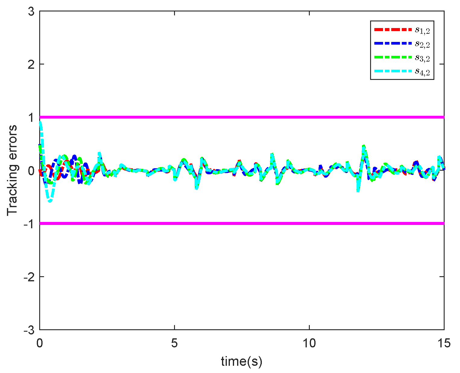
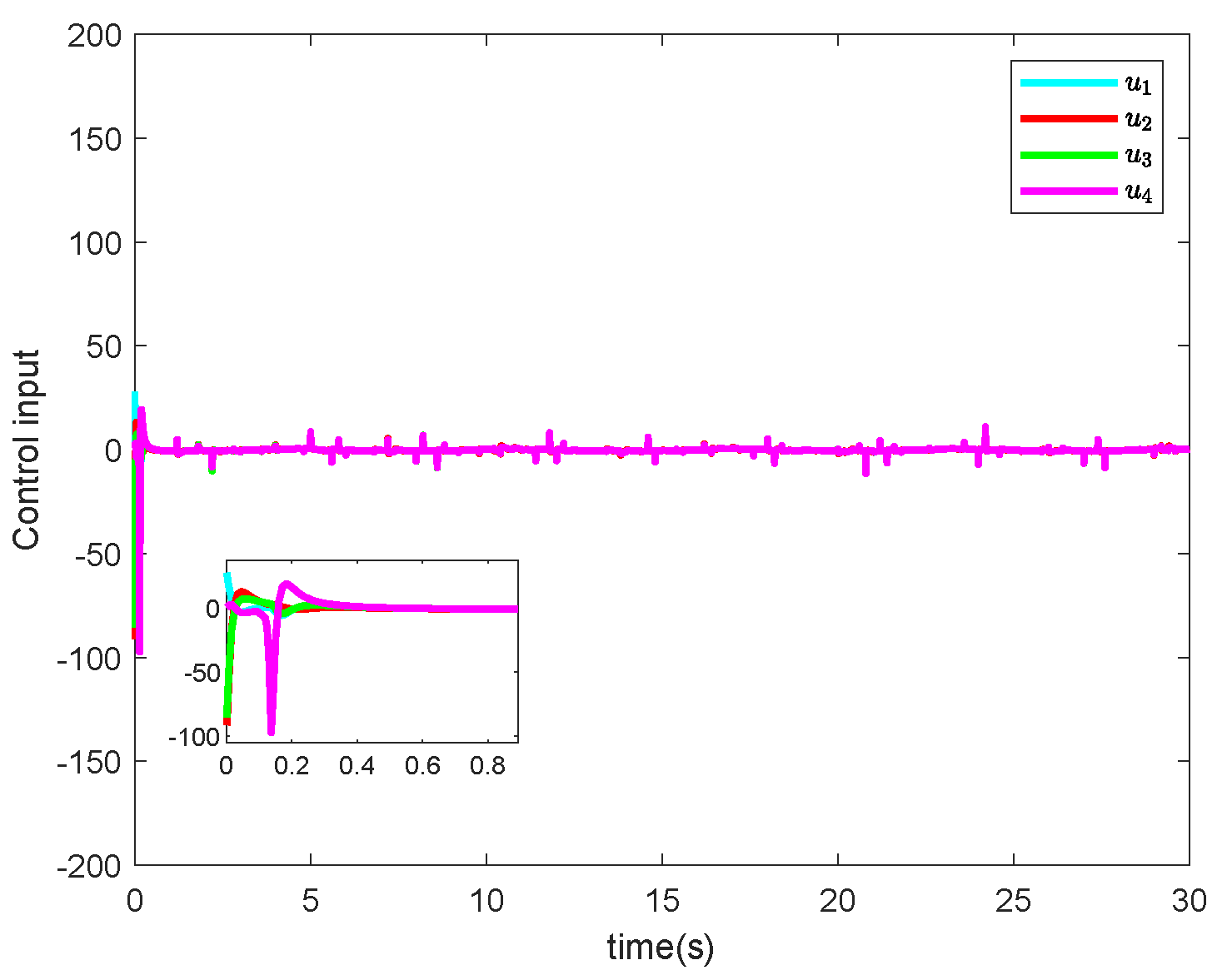
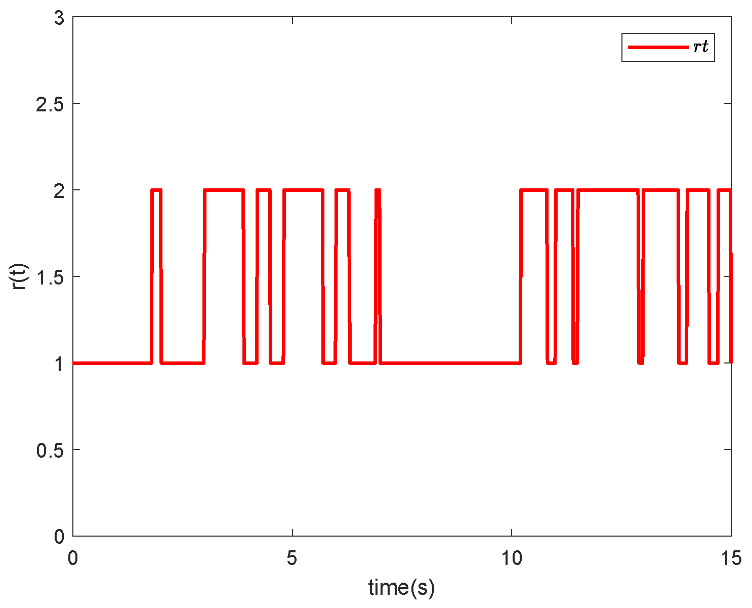
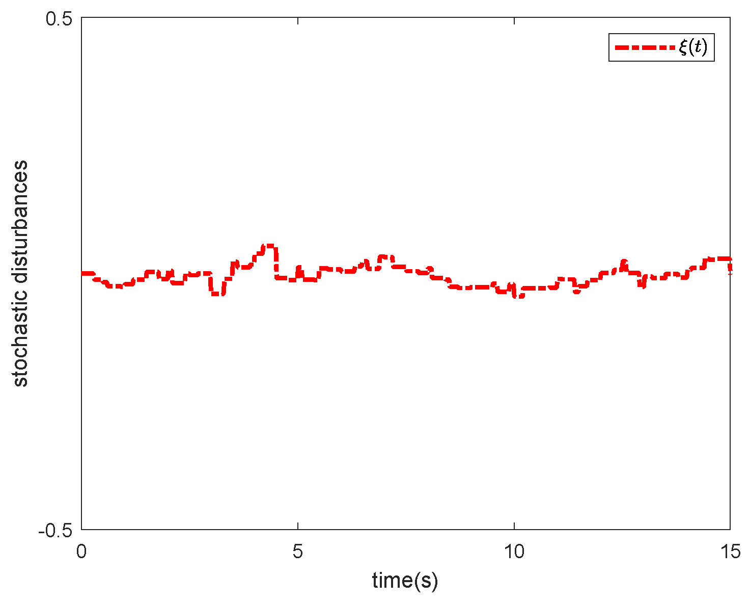
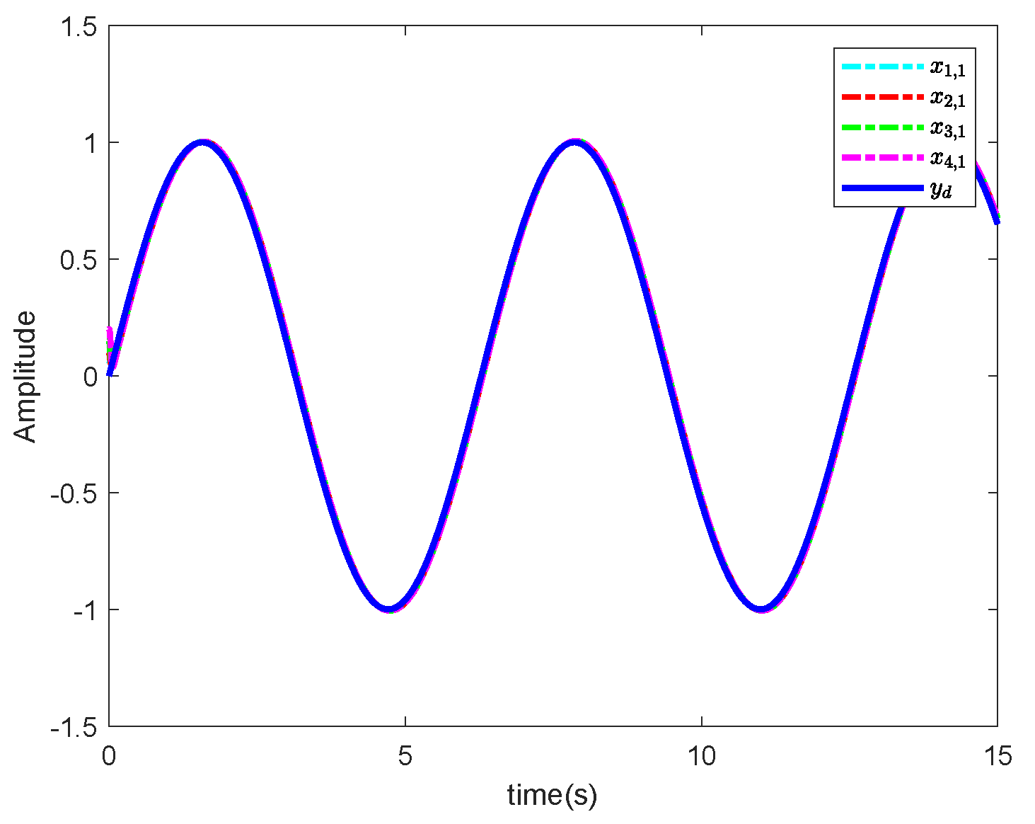
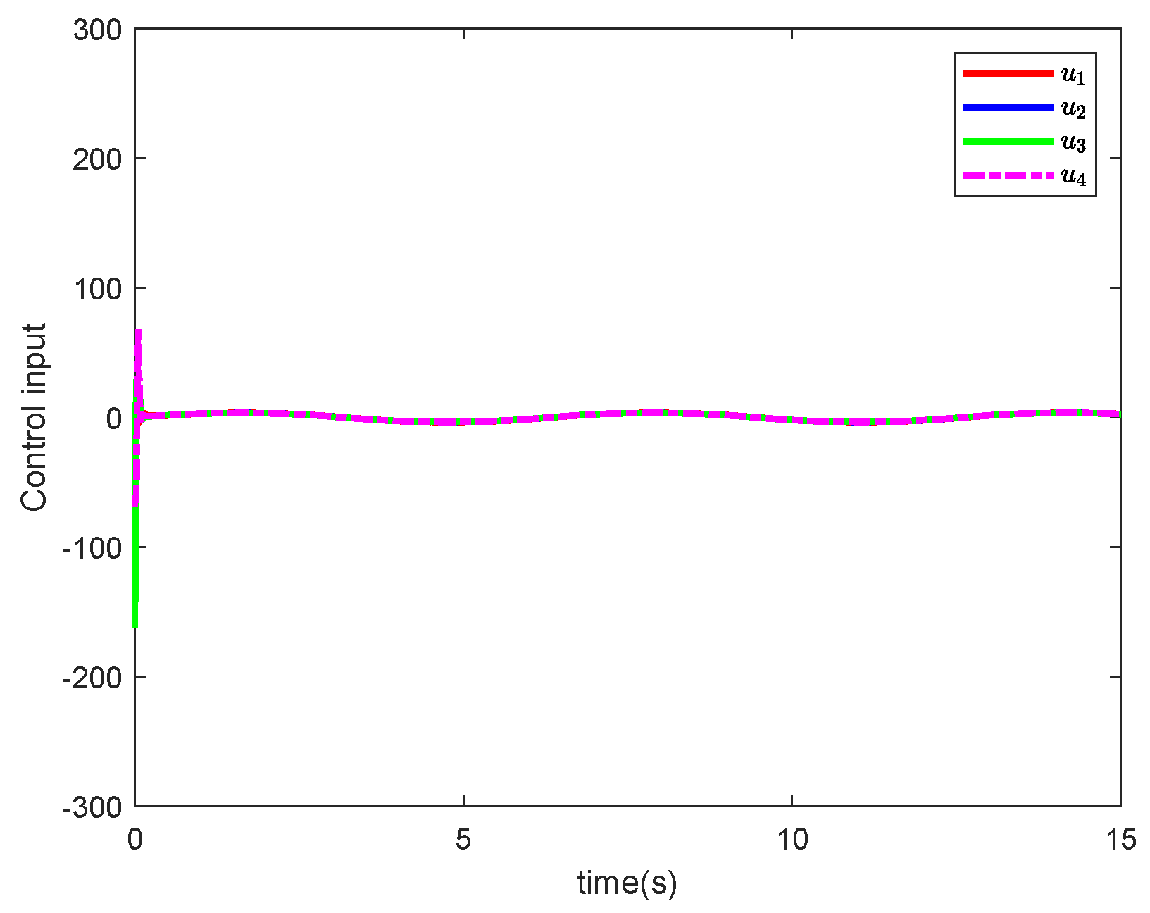
4. Simulation Example

In this section, two examples are shown to verify the effectiveness of the proposed control method for the nonlinear fractional-order Markov jump MASs with state constraints. Figure 1 illustrates the block diagram of the system controller design. Consider the MASs composed of four agents with an undirected communication topology in Figure 2. The system order is $\alpha =0.98$, and the detailed parameters in Examples 1 and 2 are listed in Table 1.

Figure 1. Block diagram of the system controller design.

Figure 2. Communication topology.

Table 1. Parameters.

Simulation Parameters	Example 1	Example 2
$c_{i,1}$	1	1
$c_{i,2}$	5	3
${\sigma }_{i,1}$	0.5	0.6
${\sigma }_{i,2}$	0.5	0.6
${\rho }_{i,1}$	1	1.5
${\rho }_{i,2}$	1	1.5
$k_{i,b1}$	0.7	0.5
$k_{i,b2}$	1	2
$d_{i,11}$	0.1	0.1
$d_{i,21}$	0.5	0.4
$d_{j,11}$	0.6	0.6
$b_i$	2	2
$v_{i,1}$	50	60
$v_{i,2}$	80	80
${\omega }_i$	0.8	0.8

Example 1. 

The dynamic of each agent is given as follows:

$$\left\{\begin{array}{c}{D}^{\alpha }{x}_{i,1}=x_{i,2}+h_{i,1}({\overline{x}}_{i,1},t,r\left(t\right))+g_{i,1}({\overline{x}}_{i,1},t,r\left(t\right)){\xi }_{i,1}\left(t\right)\hfill \\ D^{\alpha }{x}_{i,2}=u_i+h_{i,2}({\overline{x}}_{i,2},t,r\left(t\right))+g_{i,2}({\overline{x}}_{i,2},t,r\left(t\right)){\xi }_{i,2}\left(t\right)\hfill \\ y_i=x_{i,1}\hfill \end{array}\right.$$

(74)

and

$$\begin{array}{cc}\hfill & h_{i,1}=0.2r\left(t\right)\times \left(x_{i,1}+0.5x_{i,2}\right),g_{i,1}=-r\left(t\right)\times sin\left(x_{i,1}\right)\hfill \\ & h_{i,2}=0.2x_{i,1}^2+r\left(t\right)x_{i,2}^2,g_{i,2}=r\left(t\right)x_{i,1}{x}_{i,2}\hfill \end{array}$$

(75)

where $g_i({\overline{x}}_i,t,r\left(t\right))$ represents the strength coefficient of the random disturbance. Affected by Markov jump parameters, the elements in the matrix $P={\left(p_{km}\right)}_{2\times 2}$ are selected as $p_{1,1}=-4$, $p_{1,2}=4$, $p_{2,1}=3$, $p_{2,2}=-3$, then one obtains ${\tau }_1=\frac{3}{7}$, ${\tau }_2=\frac{4}{7}$. Consider that the states are constrained in $x_1$. The initial states of four agents in Figure 2 are set as $x_1\left(0\right)=[0.05,0.05]$, $x_2\left(0\right)=[0.1,0.1]$, $x_3\left(0\right)=[0.15,0.15]$, $x_4\left(0\right)=[0.2,0.2]$. The trajectory of the reference signal is $y_r=0.5\ast sin\left(t\right)$.

In this example, the stochastic processes ${\xi }_1$ and ${\xi }_2$ are generated by

$$\begin{array}{c}0.5D^{\alpha }{\xi }_1\left(t\right)=-{\xi }_1\left(t\right)+w\left(t\right)\hfill \\ 2D^{\alpha }{\xi }_2\left(t\right)=-{\xi }_2\left(t\right)+w\left(t\right)\hfill \end{array}$$

(76)

where $w\left(t\right)$ is a zero-mean white noise with $A=0.1$, ${\xi }_{i,1}\left(0\right)={\xi }_{i,2}\left(0\right)=0$, then $E{\xi }_{i,1}^2\left(t\right)=0.1$, $E{\xi }_{i,2}^2\left(t\right)=0.025$. According to the virtual controller (29), adaptive law (30)–(31), (63) and control input (62), we design

$$\begin{array}{cc}\hfill u_i& =-c_{i,2}\frac{sin\left(\frac{\pi z_{i,2}^2}{2k_{i,b2}^2}\right)cos\left(\frac{\pi z_{i,2}^2}{2k_{i,b2}^2}\right)}{z_{i,2}}-\frac{1}{2}{\omega }_{i,2}-{\theta }_{i,2}^T{\phi }_{i,2}+\frac{\partial {\alpha }_{i,1}}{\partial x_{i,1}}{x}_{j,2}+d_i\frac{\partial {\alpha }_{i,1}}{\partial x_{j,1}}{x}_{j,2}\hfill \\ & -{\widehat{r}}_{i,1}-\frac{1}{4d_{i,22}}{\varpi }_{i,2}{g_{i,2}}^2-\frac{1}{4d_{i,21}}{\left(\frac{\partial {\alpha }_{i,1}}{\partial x_{i,1}}\right)}^2{\alpha }_{i,2}{g_{i,1}}^2-\frac{1}{4d_{j,21}}{d}_i{\left(\frac{\partial {\alpha }_{i,1}}{\partial x_{j,1}}\right)}^2{\alpha }_{i,2}{g_{i,1}}^2\hfill \\ & +\frac{\partial {\alpha }_{i,1}}{\partial {\theta }_{i,1}}{D}^{\alpha }{\theta }_{i,1}\hfill \end{array}$$

(77)

and the parameters are set in Table 1.

In Example 1, Figure 3 and Figure 4 display trajectories of $r\left(t\right)$ and $\xi \left(t\right)$, which clearly show the Markov jump process between mode 1 and mode 2 and fluctuations of random noises with $E{\xi }_1^2\left(t\right)$ = 0.1 and $E{\xi }_2^2\left(t\right)=0.025$, respectively. Figure 5 shows that the outputs of four agents reach consensus, tracking the reference signal $y_d=0.5\ast sin\left(t\right)$. In Figure 6 and Figure 7, the trajectories of $s_{i,1}$ and $s_{i,2}$ are the error surfaces under the constraint of state, which are subjected to $k_{i,b1}$ and $k_{i,b2}$, respectively. The control scheme based on BLF transforms the original state constraints into a new boundary for tracking error, achieving state constraints through a constrained error surface. Figure 8 gives the trajectories of $u_i$, which shows that control inputs quickly converge to near zero. From Figure 3, Figure 4, Figure 5, Figure 6, Figure 7 and Figure 8, it can be concluded that the proposed distributed control protocol makes sure that all signals of the Markov jump FOMASs are bounded. And the tracking error in the mean-square sense can be converged to a near zero neighborhood without violating the constraints

Figure 3. The evolution of Markov process $r\left(t\right)$ in Example 1.

Figure 4. Stochastic disturbance $\xi$ in Example 1.

Figure 5. Trajectories of $x_{i,1}$ in Example 1.

Figure 6. Tracking error $s_{i,1}$ in Example 1.

Figure 7. Tracking error $s_{i,2}$ in Example 1.

Figure 8. Trajectories of control input $u_i$ in Example 1.

Example 2. 

Consider a robotic pendulum suspended from a randomly vibrating ceiling; the dynamic model is described below:

$$M_i{\ddot{\tau }}_i+{\mathrm{I}}_i\left({\tau }_i,{\dot{\tau }}_i\right)=u_i+{\Theta }_i\left({\tau }_i\right){\xi }_i$$

(78)

where ${\tau }_i$ represents the angle with vertical direction, ${\dot{\tau }}_i$ is the velocity, $u_i$ is the control input for $i=1,2,3,4$. The random force generated by the random vibration exerts an excitation on the mechanical pendulum, which is described by ${\xi }_i$, where ${\xi }_{i,1}$ and ${\xi }_{i,2}$ denote the random excitation at the reference point in the horizontal and vertical directions, respectively. The detailed parameters of the robotic pendulum are listed in Table 2.

Table 2. Parameters of robotic pendulum.

Parameter	Description	Value
${\overline{m}}_i$	the mass of load	$0.5+0.001\times {\left(-1\right)}^{r\left(t\right)}$ kg
l	length	$0.8$ m
g	the acceleration of gravity	$9.8$ m/s2

We set $M_i\left(r\left(t\right)\right)={\overline{m}}_i\left(r\left(t\right)\right)l^2$, $r\left(t\right)$ jumps between modes 1 and 2, and the elements of $P={\left(p_{km}\right)}_{2\times 2}$ are selected as $p_{1,1}=-2$, $p_{1,2}=2$, $p_{2,1}=3$, $p_{2,2}=-3$. Then, extending to the fractional-order system, we obtain $x_{i,1}={\tau }_i$, $x_{i,2}=D^{\alpha }{\tau }_i$, and system (78) can be modeled as:

$$\left\{\begin{array}{c}{D^{\alpha }x}_{i,1}=x_{i,2}\hfill \\ {D^{\alpha }x}_{i,2}=M_i^{-1}\left(r\left(t\right)\right)u_i-M_i^{-1}\left(r\left(t\right)\right)h_{i,2}+{\Theta }_{i,2}{\xi }_i\left(t\right)\hfill \end{array}\right.$$

(79)

where $h_{i,2}={\overline{m}}_i\left(r\left(t\right)\right)glsin{x}_{i,1}$, ${\Theta }_{i,2}=[-{\overline{m}}_i\left(r\left(t\right)\right)lcos{x}_{i,1},-{\overline{m}}_i\left(r\left(t\right)\right)lsin{x}_{i,1}]$, ${\xi }_i={\left[{\xi }_{i,1},{\xi }_{i,2}\right]}^T$, ${\overline{m}}_i\left(r\left(t\right)\right)=0.5+0.001\times {\left(-1\right)}^{r\left(t\right)}$ kg, $g=9.8$ m/s², $l=0.8$ m. The initial states of four agents in Figure 2 are as follows: $x_1\left(0\right)=[0.05,0.05]$, $x_2\left(0\right)=[0.1,0.1]$, $x_3\left(0\right)=[0.15,0.15]$, $x_4\left(0\right)=[0.2,0.2]$. Define $y_d=sin\left(t\right)$ as the reference signal.

The second moment stationary processes ${\xi }_1$ and ${\xi }_2$ are generated by the following dynamic equation:

$$D^{\alpha }\xi \left(t\right)=-\xi \left(t\right)+w\left(t\right)$$

(80)

where $w\left(t\right)$ is a zero-mean white noise, and its spectral function $A=0.1$, ${\xi }_{i,1}\left(0\right)={\xi }_{i,2}\left(0\right)=0$, $E{\xi }_{i,1}^2\left(t\right)=E{\xi }_{i,2}^2\left(t\right)=0.05$. According to the virtual controller ${\alpha }_{i,1}$ (29), adaptive laws (30)–(31), (63), control input $u_i$ like (77), we choose the parameters shown in Table 1. In the example, Figure 9 and Figure 10 display trajectories of $r\left(t\right)$ and $\xi \left(t\right)$, which clearly show the Markov jump process between mode 1 and mode 2 and a zero-mean widely stationary process with $E{\xi }^2\left(t\right)$ = 0.05. Figure 11 shows that the outputs of four agents reach consensus, tracking the reference signal $y_d=sin\left(t\right)$. In Figure 12, the trajectories of $s_{i,1}$ are the error surfaces under the constraint of state, which are subjected to $k_{i,b1}$. Figure 13 gives the trajectories of $u_i$ in Example 2, which shows that control inputs also quickly converge to near zero.

Figure 9. The evolution of Markov process $r\left(t\right)$ in Example 2.

Figure 10. Stochastic disturbance $\xi$ in Example 2.

Figure 11. Trajectories of $x_{i,1}$ in Example 2.

Figure 12. Tracking error $s_{i,1}$ in Example 2.

Figure 13. Trajectories of control input $u_i$ in Example 2.

5. Conclusions

This article investigates the consensus problem of random fractional-order Markov jump multi-agent systems with full state constraints. For a class of random FOMASs with Markov jump structure, an adaptive tracking controller is constructed by adopting the backstepping control method based on the neural network approximation technique. Considering the information interaction between multiple agents, in the design of the virtual control law and the control input, for each agent, we treat the partial derivative information of its neighboring agents as the unknown nonlinear term, using the ESO to address them. Through constructing the TBLF, the exponential noise-to-state stability in the mean square is analyzed rigorously, which guarantees the consensus of the considered FOMASs. Moreover, there are many related issues that deserve further research in the future, for example, how to extend the algorithms in this paper to stochastic systems containing time-delay phenomena or containing states subject to time-varying constraints, which are widely used in engineering practice.

References

1. Parivallal, A.; Sakthivel, R.; Amsaveni, R.; Alzahrani, F.; Alshomrani, A.S. Observer-based memory consensus for nonlinear multi-agent systems with output quantization and Markov switching topologies. Phys. A Stat. Mech. Its Appl. 2020, 551, 123949. [Google Scholar] [CrossRef]
2. Xu, J.; Deng, Z.; Ren, X.; Xu, L.; Liu, D. Invulnerability optimization of UAV formation based on super wires adding strategy. Chaos Solitons Fractals 2020, 140, 110185. [Google Scholar] [CrossRef]
3. Wang, Y.; Wang, Z.; Chen, M.; Kong, L. Predefined-time sliding mode formation control for multiple autonomous underwater vehicles with uncertainties. Chaos Solitons Fractals 2021, 144, 110680. [Google Scholar] [CrossRef]
4. Kauffman, S.A. Metabolic stability and epigenesis in randomly constructed genetic nets. J. Theor. Biol. 1969, 22, 437–467. [Google Scholar] [CrossRef]
5. Goles, E.; Medina, P.; Montealegre, P.; Santivañez, J. Majority networks and consensus dynamics. Chaos Solitons Fractals 2022, 164, 112697. [Google Scholar] [CrossRef]
6. Wang, W.; Yin, X.; Cao, Y.; Jiang, L.; Li, Y. A distributed cooperative control based on consensus protocol for VSC-MTDC systems. IEEE Trans. Power Syst. 2021, 36, 2877–2890. [Google Scholar] [CrossRef]
7. Gao, Y.; Liu, B.; Yu, J.; Ma, J.; Jiang, T. Consensus of first-order multi-agent systems with intermittent interaction. Neurocomputing 2014, 129, 273–278. [Google Scholar] [CrossRef]
8. Ma, Z.; Wang, Y.; Li, X. Cluster-delay consensus in first-order multi-agent systems with nonlinear dynamics. Nonlinear Dyn. 2016, 83, 1303–1310. [Google Scholar] [CrossRef]
9. Hou, W.; Fu, M.; Zhang, H.; Wu, Z. Consensus conditions for general second-order multi-agent systems with communication delay. Automatica 2017, 75, 293–298. [Google Scholar] [CrossRef]
10. Miao, G.; Xu, S.; Zhang, B.; Zou, Y. Mean square consensus of second-order multi-agent systems under Markov switching topologies. IMA J. Math. Control Inf. 2014, 31, 151–164. [Google Scholar] [CrossRef]
11. Li, W.; Zhang, J.F. Distributed practical output tracking of high-order stochastic multi-agent systems with inherent nonlinear drift and diffusion terms. Automatica 2014, 50, 3231–3238. [Google Scholar] [CrossRef]
12. Zhou, H.; Sui, S.; Tong, S. Fuzzy adaptive finite-time consensus control for high-order nonlinear multiagent systems based on event-triggered. IEEE Trans. Fuzzy Syst. 2022, 30, 4891–4904. [Google Scholar] [CrossRef]
13. Jiang, J.; Jiang, Y. Leader-following consensus of linear time-varying multi-agent systems under fixed and switching topologies. Automatica 2020, 113, 108804. [Google Scholar] [CrossRef]
14. Krasovskii, N.; Lidskii, E. Analytical design of controllers in systems with random attributes. Autom. Remote Control 1961, 22, 1021–1025. [Google Scholar]
15. Benjelloun, K.; Boukas, E.K. Stochastic stability of linear time-delay system with Markovian jumping parameters. Math. Probl. Eng. 1997, 3, 187–201. [Google Scholar] [CrossRef]
16. Drǎgan, V.; Shi, P.; Boukas, E.K. Control of singularly perturbed systems with Markovian jump parameters: An H infinity approach. Automatica 1999, 35, 1369–1378. [Google Scholar] [CrossRef]
17. Li, W.; Wu, Z. Output tracking of stochastic high-order nonlinear systems with Markovian switching. IEEE Trans. Autom. Control 2012, 58, 1585–1590. [Google Scholar] [CrossRef]
18. Wu, Z.J.; Yang, J.; Shi, P. Adaptive tracking for stochastic nonlinear systems with markovian switching. IEEE Trans. Autom. Control 2010, 55, 2135–2141. [Google Scholar] [CrossRef]
19. Wang, D.; Wang, Z.; Wu, Z.; Wang, W. Distributed convex optimization for nonlinear multi-agent systems disturbed by a second-order stationary process over a digraph. Sci. China Inf. Sci. 2022, 65, 132201. [Google Scholar] [CrossRef]
20. Liu, S.; Niu, B.; Zong, G.; Zhao, X.; Xu, N. Adaptive neural dynamic-memory event-triggered control of high-order random nonlinear systems with deferred output constraints. IEEE Trans. Autom. Sci. Eng. 2023. [Google Scholar] [CrossRef]
21. Yao, L.; Zhang, W. Adaptive tracking control for a class of random pure-feedback nonlinear systems with Markovian switching. Int. J. Robust Nonlinear Control 2018, 28, 3112–3126. [Google Scholar] [CrossRef]
22. Jiao, T.; Lu, J.; Li, Y.; Chu, Y.; Xu, S. Stability analysis of random systems with Markovian switching and its application. J. Frankl. Inst. 2016, 353, 200–220. [Google Scholar] [CrossRef]
23. Xu, Z.; Zhou, X.; Dong, Z.; Hu, X.; Sun, C.; Shen, H. Observer-based prescribed performance adaptive neural output feedback control for full-state-constrained nonlinear systems with input saturation. Chaos Solitons Fractals 2023, 173, 113593. [Google Scholar] [CrossRef]
24. Wu, J.; Qin, G.; Cheng, J.; Cao, J.; Yan, H.; Katib, I. Adaptive neural network control for Markov jumping systems against deception attacks. Neural Netw. 2023, 168, 206–213. [Google Scholar] [CrossRef]
25. Zhang, Y.; Sun, J.; Liang, H.; Li, H. Event-triggered adaptive tracking control for multiagent systems with unknown disturbances. IEEE Trans. Cybern. 2018, 50, 890–901. [Google Scholar] [CrossRef]
26. Wang, Z.; Yuan, Y.; Yang, H. Adaptive fuzzy tracking control for strict-feedback Markov jumping nonlinear systems with actuator failures and unmodeled dynamics. IEEE Trans. Cybern. 2018, 50, 126–139. [Google Scholar] [CrossRef] [PubMed]
27. Wang, Z.; Yuan, J.; Pan, Y.; Che, D. Adaptive neural control for high order Markovian jump nonlinear systems with unmodeled dynamics and dead zone inputs. Neurocomputing 2017, 247, 62–72. [Google Scholar] [CrossRef]
28. Zhao, L.; Yu, J.; Shi, P. Adaptive finite-time command filtered backstepping control for Markov jumping nonlinear systems with full-state constraints. IEEE Trans. Circuits Syst. II Express Briefs 2022, 69, 3244–3248. [Google Scholar] [CrossRef]
29. Hu, A.; Cao, J.; Hu, M.; Guo, L. Event-triggered consensus of Markovian jumping multi-agent systems via stochastic sampling. IET Control Theory Appl. 2015, 9, 1964–1972. [Google Scholar] [CrossRef]
30. Luo, X.; Wang, J.; Feng, J.; Cai, J.; Zhao, Y. Dynamic Event-Triggered Consensus Control for Markovian Switched Multi-Agent Systems: A Hybrid Neuroadaptive Method. Mathematics 2023, 11, 2196. [Google Scholar] [CrossRef]
31. Sakthivel, R.; Parivallal, A.; Kaviarasan, B.; Lee, H.; Lim, Y. Finite-time consensus of Markov jumping multi-agent systems with time-varying actuator faults and input saturation. ISA Trans. 2018, 83, 89–99. [Google Scholar] [CrossRef]
32. Ni, H.; Xu, Z.; Cheng, J.; Zhang, D. Robust stochastic sampled-data-based output consensus of heterogeneous multi-agent systems subject to random DoS attack: A Markovian jumping system approach. Int. J. Control. Autom. Syst. 2019, 17, 1687–1698. [Google Scholar] [CrossRef]
33. Wu, L.B.; Park, J.H.; Xie, X.P.; Ren, Y.W.; Yang, Z. Distributed adaptive neural network consensus for a class of uncertain nonaffine nonlinear multi-agent systems. Nonlinear Dyn. 2020, 100, 1243–1255. [Google Scholar] [CrossRef]
34. Chen, T.; Yuan, J. Command-filtered adaptive containment control of fractional-order multi-agent systems via event-triggered mechanism. Trans. Inst. Meas. Control 2023, 45, 1646–1660. [Google Scholar] [CrossRef]
35. Yang, X.; Yuan, J.; Chen, T.; Yang, H. Distributed Adaptive Optimization Algorithm for Fractional High-Order Multiagent Systems Based on Event-Triggered Strategy and Input Quantization. Fractal Fract. 2023, 7, 749. [Google Scholar] [CrossRef]
36. Yuan, J.; Chen, T. Switched fractional order multiagent systems containment control with event-triggered mechanism and input quantization. Fractal Fract. 2022, 6, 77. [Google Scholar] [CrossRef]
37. Tee, K.P.; Ge, S.S.; Tay, E.H. Barrier Lyapunov functions for the control of output-constrained nonlinear systems. Automatica 2009, 45, 918–927. [Google Scholar] [CrossRef]
38. Liu, Y.J.; Tong, S. Barrier Lyapunov functions-based adaptive control for a class of nonlinear pure-feedback systems with full state constraints. Automatica 2016, 64, 70–75. [Google Scholar] [CrossRef]
39. Wang, Y.; Jiang, X.; She, W.; Ding, F. Tracking control with input saturation and full-state constraints for surface vessels. IEEE Access 2019, 7, 144741–144755. [Google Scholar] [CrossRef]
40. Wang, C.; Wang, F.; Yu, J. BLF-based asymptotic tracking control for a class of time-varying full state constrained nonlinear systems. Trans. Inst. Meas. Control 2019, 41, 3043–3052. [Google Scholar] [CrossRef]
41. Chen, T.; Yuan, J.; Yang, H. Event-triggered adaptive neural network backstepping sliding mode control of fractional-order multi-agent systems with input delay. J. Vib. Control 2022, 28, 3740–3766. [Google Scholar] [CrossRef]
42. Gao, C.; Wang, Z.; He, X.; Han, Q.L. Consensus control of linear multiagent systems under actuator imperfection: When saturation meets fault. IEEE Trans. Syst. Man Cybern. Syst. 2021, 52, 2651–2663. [Google Scholar] [CrossRef]
43. Li, Y.; Chen, Y.; Podlubny, I. Mittag–Leffler stability of fractional order nonlinear dynamic systems. Automatica 2009, 45, 1965–1969. [Google Scholar] [CrossRef]
44. Podlubny, I. Fractional Differential Equations: An Introduction to Fractional Derivatives, Fractional Differential Equations, to Methods of Their Solution and Some of Their Applications; Elsevier: Amsterdam, The Netherlands, 1998. [Google Scholar]
45. Meyn, S.P.; Tweedie, R.L. Markov Chains and Stochastic Stability; Springer Science & Business Media: Berlin/Heidelberg, Germany, 2012. [Google Scholar]
46. Liu, Y.; Zhu, Q.; Zhao, N.; Wang, L. Adaptive fuzzy backstepping control for nonstrict feedback nonlinear systems with time-varying state constraints and backlash-like hysteresis. Inf. Sci. 2021, 574, 606–624. [Google Scholar] [CrossRef]
47. Gharesifard, B.; Cortés, J. Distributed continuous-time convex optimization on weight-balanced digraphs. IEEE Trans. Autom. Control 2013, 59, 781–786. [Google Scholar] [CrossRef]
48. Yang, Y.; Si, X.; Yue, D.; Tian, Y.C. Time-varying formation tracking with prescribed performance for uncertain nonaffine nonlinear multiagent systems. IEEE Trans. Autom. Sci. Eng. 2020, 18, 1778–1789. [Google Scholar] [CrossRef]
49. Ross, S.M. Stochastic Processes; John Wiley & Sons: Hoboken, NJ, USA, 1995. [Google Scholar]