Article

On Theoretical and Numerical Results of Serum Hepatitis Disease Using Piecewise Fractal–Fractional Perspectives

by
Zareen A. Khan
1,*,
Arshad Ali
2,*,
Ateeq Ur Rehman Irshad
3,
Burhanettin Ozdemir
3 and
Hussam Alrabaiah
4,5
1
Department of Mathematical Sciences, College of Science, Princess Nourah bint Abdulrahman University, P.O. Box 84428, Riyadh 11671, Saudi Arabia
2
Department of Mathematics, University of Malakand, Chakdara 18000, Khyber Pakhtunkhwa, Pakistan
3
Department of Mathematics and Sciences, Prince Sultan University, P.O. Box 11586, Riyadh 12435, Saudi Arabia
4
College of Engineering, Al Ain University, Al Ain 112612, United Arab Emirates
5
Mathematics Department, Tafila Technical University, Tafila 66110, Jordan
*
Authors to whom correspondence should be addressed.
Fractal Fract. 2024, 8(5), 260; https://doi.org/10.3390/fractalfract8050260
Submission received: 21 March 2024 / Revised: 9 April 2024 / Accepted: 23 April 2024 / Published: 26 April 2024

Abstract

:
In the present research, we consider a biological model of serum hepatitis disease. We carry out a detailed analysis of the mentioned model along with a class with asymptomatic carriers to explore its theoretical and numerical aspects. We initiate the study by using the piecewise fractal–fractional derivative (FFD) by which the crossover effects within the model are examined. We split the time interval into subintervals. In one subinterval, FFD with a power law kernel is taken, while in the second one, FFD with an exponential decay kernel of the proposed model is considered. This model is then studied for its disease-free equilibrium point, existence, and Hyers–Ulam (H-U) stability results. For numerical results of the model and a visual presentation, we apply the Lagrange interpolation method and an extended Adams–Bashforth–Moulton (ABM) method, respectively.

1. Introduction

Serum hepatitis, also known as Hepatitis B, is a serious disease that causes liver infection. This disease is caused by the Hepatitis B virus (HBV) and poses a significant health challenge worldwide. It can lead to both acute (short-term) and chronic (long-term) illnesses. Initially, it may be transmitted to a child from an infected mother before his/her birth (pregnancy period) and during delivery or childbirth. Its spread also takes place from an infected individual via sexual contact, through contact with the blood of an infected individual, or through unsafe injections. Its transmission may take place via contact with poisonous or polluted medical equipment or other objects. Similarly, injection practices can be a reason for its transmission. As claimed by the World Health Organization (WHO), about 296 million individuals globally are living with chronic infection. It is reported that in 2019, around 820,000 people died from this infection, with the majority of deaths attributed to cirrhosis and hepatocellular carcinoma (primary liver cancer). Moreover, 22% of the diagnosed population, which is almost 6.6 million individuals, were medically treated. This number makes up almost 10% of infected people.
The WHO reported a significant decline in the spread of chronic infection among children under five years of age. During the pre-vaccination period from the 1980s to the 2000s, the estimated rate was about 5%, whereas in 2019, it was less than 1%. However, we should note that the WHO predicts almost 1.5 million new cases of this serious disease every year. Preventive measures include antiviral prophylaxis during pregnancy, as well as safe and effective vaccinations. These interventions are of great importance in the prevention and control of Hepatitis B. The HBV models studied in the sense of classical derivatives are unable to capture memory and genetic characteristics, which can be observed in non-integer-order models.
Researchers and mathematicians have focused on fractional calculus due to its effective use in the modeling of various mathematical problems in many real-world situations. More specifically, researchers working in applied mathematics have taken an interest in non-integer-order derivatives to achieve higher accuracy in mathematical modeling (see [1,2,3,4,5,6,7]). Fractional calculus [8,9] is continuously being developed to more deeply and accurately understand the properties of real-world problems. It allows researchers in this field to analyze and explore phenomena that cannot be described accurately by integer-order calculus. Complex systems and phenomena can be better understood by using fractional derivatives and integrals. The advancements in fractional order calculus offer opportunities to enhance our understanding of real-world problems. In recent literature, various types of non-integer-order differential operators, along with their associated integral operators, have been explored. Caputo and Fabrizio [10] investigated non-integer-order derivatives with the exponential kernel. In [11], authors investigated properties of the new fractional derivative without singular kernel. Atangana and Baleanu [12] formulated fractional derivatives and integrals with Mittag-Leffler kernels and extended them to higher arbitrary orders.
In some real-world phenomena, transitions are observed when they shift from power law to exponential decay, or from deterministic to stochastic randomness. Atangana and Araz [13] proposed a new concept of piecewise differential and integral operators, which are effective for modeling and solving such phenomena. This approach is not like conventional methods, which do not exhibit crossover behavior due to their lack of abrupt changes. Additionally, the time interval is split into two subintervals at the point of discontinuity. In contrast to the usual fractional derivatives, the piecewise concept is useful in describing these crossover effects among various forms (see [14]).
On the other hand, researchers have focused on fractal–fractional calculus due to its significant use in real-world problems. The idea of fractal–fractional was formally started a few years ago when the author of reference [15] published the first work about this. The concept of fractals is as old as fractional calculus. Researchers have used the applications of fractal–fractional to investigate various problems in physical sciences. For instance, see [16,17]. For more applications, see [18,19].
Gul et al. [20] considered the HBV model. They studied the dynamics of the Caputo fractional order HBV model with asymptomatic carriers. They studied the existence, stability results, and numerical solution of the considered model and simulated the results. In [21], the authors investigated this model under the piecewise Atangana Baleanu derivative and derived the aforementioned results. In both research studies, the authors made significant efforts toward accurate modeling of the disease; however, these models lack a memory effect. As with many real-world problems, it is necessary to know how much information a system carries. In such a situation, the concept of a fractal–fractional derivative is beneficial. In our research paper, we reformulate the HBV model in the sense of the piecewise fractal–fractional order derivative, which incorporates the additional property of memory and manages the crossover effect. In this sense, our proposed model is more informative. Moreover, typically in a piecewise derivative, a classical derivative is taken in the first subinterval of the time domain with the concerned fractional derivative in the second subinterval. In our paper, we consider an FFD with a power law kernel in the first subinterval and an FFD with an exponential decay kernel in the second subinterval. This makes the results more interesting and different.
The innovations and objectives of this research are as follows:
  • To define a piecewise Caputo FFD by combining the FFD with the power law kernel and FFD with the exponential decay-type kernel.
  • To reformulate serum hepatitis disease in the sense of piecewise Caputo FFD.
  • To study the existence and H-U type stability results for the proposed model under piecewise Caputo FFD.
  • To find the numerical solution of the proposed model under piecewise Caputo FFD by applying the Lagrange interpolation method and the extended ABM method.
  • To visually present our results.
The rest of the manuscript is structured as follows: In Section 2, we present the basic definitions and preliminary results. In Section 3, the proposed mathematical model and its formulation are presented. Section 4 is allocated to the derivation of the basic reproduction number of the concerned model. In Section 5, we analyze the fractional order system, derive the main results of existence, and present the uniqueness of the solution along with their stability results based on H-U’s concept of stability. In Section 6, the computational results along with graphical representations of the proposed model are presented. In Section 7, we present the conclusion of the main work with some future work directions.

2. Basic Results

Definitions 1 and 2 are adopted from [13]. In the upcoming definitions, ς denotes the fractional order derivative while η denotes the fractal dimension.
Definition 1.
For y C [ 0 , T ] and 0 < ς , η 1 , the piecewise Caputo-fractal–fractional derivative is defined by
D ς , η P C F F y ( t ) = D p ς , η C F F y ( t ) , t [ 0 , t 1 ] , D e ς , η C F F y ( t ) , t ( t 1 , T ] ,
where the notion D p ς , η C F F y ( t ) represents FFD with the power law kernel while the notion D e ς , η C F F y ( t ) represents FFD with the exponential decay-type kernel.
Definition 2.
Let y C ( 0 , T ) . Then, we define the ςth order piecewise fractal–fractional integral (FFI) of y ( t ) as follows:
I ς , η P F F y ( t ) = I p ς , η F F y ( t ) , t [ 0 , t 1 ] , I e ς , η F F y ( t ) , t ( t 1 , T ] ;
I p ς , η F F y ( t ) and I e ς , η F F y ( t ) are defined bellow.
Definition 3
([15]). Let y C ( 0 , T ) . Then, the FFI of y associated with the power law kernel is defined as follows:
I p ς , η F F y ( t ) = η Γ ( ς ) 0 t v η 1 ( t v ) ς 1 y ( v ) d v .
Definition 4
([15]). Let y C ( 0 , T ) . Then, the FFI of y ( t ) associated with the exponential decay kernel is defined as follows:
I e ς , η 0     F F y ( t ) = η ( 1 ς ) t η 1 y ( t ) B ( ς ) + ς η B ( ς ) a t v ς 1 y ( v ) d v .
Definition 5
([15]). For y C [ 0 , T ] and 0 < ς , η 1 , if y is fractal-differentiable on ( a , b ) with the order of η , then FFD with the power law kernel is defined as follows:
D p ς , η C F F y ( t ) = 1 Γ ( 1 ς ) d d t η 0 t ( t v ) ς d v .
Definition 6
([15]). For 0 ς , η 1 , the FFD of y with the exponential decay kernel is given by the following:
D e ς , η 0       C F F y ( t ) = B ( ς ) 1 ς d d t η a t exp ς ( t v ) α ς 1 1 ς y ( z ) d v ,
where M ( 0 ) = M ( 1 ) = 1 .
Theorem 1.
If Q 1 , Q 2 are two operators such that the first is a contraction and the second is completely continuous over a closed bounded subset H of a Banach space J, then the operator equation Q F + Q 2 F = F has at least one solution.
Definition 7.
The formula used for the Adams–Bashforth method of ordinary problems is given by the following:
y m + 1 = y m + h i = 1 r b i f ( x m + i h , y m + i h ) ,
where
  • y m is the approximate solution at time x m .
  • h is the step size.
  • f ( y , x ) is the ODE.
  • b i are coefficients that depend on the order of the method.

3. Mathematical Model and Its Formulation

This section is subdivided into two subsections, where the mathematical model and its formulation are presented, respectively.

3.1. Mathematical Model

We generalize the HBV model [20] in the sense of the piecewise FFD with the power law kernel and the exponential law kernel as follows:
D t ς , η P C F F X ( t ) = ϱ ϑ A + ω 1 A c + 1 C X ξ X , X ( 0 ) > 0 , D t ς , η P C F F E ( t ) = ϑ A + ω 1 A c + 1 C X ξ + ψ 1 E , E ( 0 ) > 0 , D t ς , η P C F F A ( t ) = ψ 1 n E ξ + μ + ρ 1 + η 1 A , A ( 0 ) > 0 , D t ς , η P C F F A c ( t ) = ψ 1 1 n E ξ + x 1 + λ A c , A c ( 0 ) > 0 , D t ς , η P C F F C ( t ) = ρ 1 A + x 1 A c ξ + δ + v 1 C , C ( 0 ) > 0 , D t ς , η P C F F R p ( t ) = η 1 A + v 1 C + λ A c ξ R p , R p ( 0 ) > 0 ;
ϱ is the susceptible birth rate, and ϑ and ξ denote the effective contact rate and natural fatality rate, respectively. ψ 1 1 n is the infection rate of the exposed population, with a portion of ψ 1 1 n , shifting to class A at a rate of ψ 1 n . Class A c is used for symptomatically infected individuals. ρ 1 and x 1 denote the rates at which individuals of acute and asymptomatic classes become carriers, respectively. η 1 , λ , and v 1 denote the recovery rates for acute, asymptomatic, and carrier individuals, respectively. μ and δ denote the death rates in the acute and chronic classes due to disease, respectively. ω 1 and 1 denote the coefficients of asymptomatic and carrier individuals, respectively.

3.2. Model Formulation

In deriving the integer-order model of serum hepatitis disease, we take the total human population, N ( t ) as a sum of six classes; that is, N ( t ) = X ( t ) + E ( t ) + A ( t ) + A c ( t ) + C ( t ) + R p ( t ) , where the parameters are defined in Table 1.
Susceptible class: The class X ( t ) is recruited at the rate ϱ and decreased due to the natural fatality (death) rate ξ . Also, this class diminishes as a proportion of the population becomes infected after contact with either Class A of acutely infected individuals or the asymptomatic carrier and chronic class C ( t ) of infected individuals, at rates of ω 1 and 1 , respectively. Therefore, we formulated the dynamics of the susceptible class of individuals, as follows:
d X ( t ) d t = ϱ ϑ A + ω 1 A c + 1 C X ξ X .
Exposed class: Class E ( t ) increases at the rate ϑ , which represents the proportion of the population becoming newly infected through previously described contacts. This class decreases due to the natural fatality rate, ξ , and by the rate at which the exposed population becomes acutely infected. Therefore, we formulate the dynamics of the exposed class of the population as follows:
d E ( t ) d t = ϑ A + ω 1 A c + 1 C X ξ + ψ 1 E .
Acute class: Class A ( t ) is recruited at the rate ψ 1 n of the exposed population. This class decreases at the natural fatality rate, ξ , by the death rate, μ , due to disease in the acute class. This class also decreases by the rate ρ 1 , at which the individuals of the class go to the asymptomatic carrier, and by the rate η 1 , at which the individuals of the class recover. Therefore, we formulate the dynamics of the acute class of the population as follows:
d A ( t ) d t = ψ 1 n E ξ + μ + ρ 1 + η 1 A .
Asymptomatic carrier: Class A c ( t ) is recruited from the exposed class at the rate ψ 1 and decreases at the rate ψ 1 n , which represents the transition of individuals from the exposed to the acute class. This class decreases due to the natural fatality rate ξ , the rate, x 1 , at which members transition to the chronic class of infected individuals. Also, it decreases at the rate λ , at which members of the class recover. Therefore, we formulate the dynamics of the asymptomatic carrier as follows:
d A c ( t ) d t = ψ 1 1 n E ξ + x 1 + λ A c .
Chronic class of infected individuals: Class C ( t ) is recruited at the rates of ρ 1 and x 1 of the acute class of infected individuals and asymptomatic carriers, respectively. The class is reduced by the natural fatality rate, ξ , as well as the δ fatality rate, due to disease. The class also reduces by the rate, v 1 , at which the individuals in the class recover. Therefore, we formulate the dynamics of the chronic class of infected individuals as follows:
d C ( t ) d t = ρ 1 A + x 1 A c ξ + δ + v 1 C .
Recovered class of individuals: Class R p ( t ) grows at rates η 1 , v 1 , and λ , where the individuals of the aforementioned classes recover and decrease at a natural fatality rate, ξ . Therefore, we formulate the dynamics of a recovered class of individuals as follows:
d R p ( t ) d t = η 1 A + v 1 C + λ A c ξ R p .
As a result of the above derivations of the aforementioned classes, the integer-order model of serum hepatitis disease with a class of asymptomatic carriers is presented as follows:
d X ( t ) d t = ϱ ϑ A + ω 1 A c + 1 C X ξ X , X ( 0 ) > 0 , d E ( t ) d t = ϑ A + ω 1 A c + 1 C X ξ + ψ 1 E , E ( 0 ) > 0 , d A ( t ) d t = ψ 1 n E ξ + μ + ρ 1 + η 1 A , A ( 0 ) > 0 , d A c ( t ) d t = ψ 1 1 n E ξ + x 1 + λ A c , A c ( 0 ) > 0 , d C ( t ) d t = ρ 1 A + x 1 A c ξ + δ + v 1 C , C ( 0 ) > 0 , d R p ( t ) d t = η 1 A + v 1 C + λ A c ξ R p , R p ( 0 ) > 0 .
We extend the integer-order model presented in (7) to a piecewise fractal–fractional order model with power law and exponential law kernels as given in (6).

4. Equilibrium Point and Basic Reproduction Number

For disease-free equilibrium point Θ 0 , we have the following:
ϱ ϑ A + ω 1 A c + 1 C X ξ X = 0 ϑ A + ω 1 A c + 1 C X ξ + ψ 1 E = 0 ψ 1 n E ξ + μ + ρ 1 + η 1 A = 0 ψ 1 1 n E ξ + x 1 + λ A c = 0 ρ 1 A + x 1 A c ξ + δ + v 1 C = 0 η 1 A + v 1 C + λ A c ξ R p = 0 .
And is provided as follows:
Θ 0 = ϱ ξ , 0 , 0 , 0 , 0 , 0 ;
ϱ is the birth rate of the affected population and ξ denotes the natural dying rate, respectively. From [22], the basic reproduction number, R 0 , for model (6) is given by the following:
R 0 = ϑ ϱ n ψ 1 ξ θ 2 θ 1 + ϑ ω 1 ϱ ψ 1 1 n ξ θ 3 θ 1 + ϑ 1 ϱ ρ 1 n ψ 1 ξ θ 4 θ 1 θ 2 + ϑ x 1 ϱ ψ 1 1 1 n ξ θ 4 θ 3 θ 1 ,
where
θ 1 = ξ + ψ 1 , θ 2 = ξ + μ + ρ 1 + η 1 , θ 3 = ξ + x 1 + λ , θ 4 = ξ + δ + v 1 .

Significance of the Basic Reproduction Number

The basic reproduction number is the average number of infected contacts per sick individual. It is a dimensionless number rather than a rate. Therefore, R 0 is the number of secondary infections produced by a single typical infection in a rarefied population. It plays an important role in predicting the infection in society. If there are no environmental changes or outside factors that intervene, a virus will continue to spread among susceptible hosts at the population level if R 0 is greater than 1.

5. Existence and Stability Analysis of the Piecewise Fractal–Fractional Model 6

In this section, the main results, such as the existence, uniqueness, and stability of the solution of the proposed model (6), are established. Let I = 0 , T . We define a Banach space as follows: J = C I , R + × C I , R + × C I , R + × C I , R + × C I , R + × C I , R + under the given norm, as follows:
s = sup X ( t ) + E ( t ) + A ( t ) + A c ( t ) + C ( t ) + R P ( t ) ;
X , E , A , A c , C , R P J .
Lemma 1.
The piecewise-fractal–fractional problem is as follows:
D p ς , η C F F s ( t ) = φ ( t ) , 0 < ς , η 1 , i f   t 0 , t 1 , s ( 0 ) = s 0 , D e ς , η C F F s ( t ) = φ ( t ) , 0 < ς , η 1 , i f   t t 1 , T , s ( t 1 ) = s 1 ,
has the following solution:
s ( t ) = s 0 + η Γ ( ς ) 0 t 1 v η 1 ( x v ) ς 1 φ ( v ) d v , i f   t 0 , t 1 , s ( t 1 ) + ( 1 ς ) B ( ς ) η t η 1 φ ( t ) + ς η B ( ς ) t 1 t v η 1 φ ( v ) d v , i f   t t 1 , T .
We reformulate model (6) as follows:
D ς , η P C F F X ( t ) = Φ 1 ( t , s ( t ) ) , D ς , η P C F F E ( t ) = Φ 2 ( t , s ( t ) ) , D ς , η P C F F A ( t ) = Φ 3 ( t , s ( t ) ) , D ς , η P C F F A C ( t ) = Φ 4 ( t , s ( t ) ) , D ς , η P C F F C ( t ) = Φ 5 ( t , s ( t ) ) , D ς , η P C F F R p ( t ) = Φ 6 ( t , s ( t ) ) ,
where
Φ 1 ( t , s ( t ) ) = ϱ ϑ A + ω 1 A c + 1 C X ξ X , Φ 2 ( t , s ( t ) ) = ϑ A + ω 1 A c + 1 C X ξ + ψ 1 E , Φ 3 ( t , s ( t ) ) = ψ 1 n E ξ + μ + ρ 1 + η 1 A , Φ 4 ( t , s ( t ) ) = ψ 1 1 n E ξ + x 1 + λ A c , Φ 5 ( t , s ( t ) ) = ρ 1 A + x 1 A c ξ + δ + v 1 C , Φ 6 ( t , s ( t ) ) = η 1 A + v 1 C + λ A c ξ R p .
We take our model as follows:
D ς , η P C F F s ( t ) = F ( t , s ( t ) ) , s ( 0 ) = s 0 > 0 .
In view of Definitions 2 and 3 and Lemma 1, the equivalent form of model (10) is given by the following:
s ( t ) = s 0 + η Γ ( ς ) 0 t v η 1 ( t v ) ς 1 F ( v , s ( v ) ) d v , i f   t 0 , t 1 , s ( t 1 ) + ( 1 ς ) B ( ς ) η t η 1 F ( t , s ( t ) ) + ς η B ( ς ) t 1 t v η 1 F ( v , s ( v ) ) d v , i f   t t 1 , T .
where
s ( t ) = X ( t ) E ( t ) A ( t ) A c ( t ) C ( t ) R p ( t ) , s ( 0 ) = X 0 E 0 A 0 A c C 0 R p 0 , s ( t 1 ) = X t 1 E t 1 A t 1 A c C t 1 R p t 1 .
and
F ( t , s ( t ) ) = Φ 1 ( t , s ( t ) ) Φ 2 ( t , s ( t ) ) Φ 3 ( t , s ( t ) ) Φ 4 ( t , s ( t ) ) Φ 5 ( t , s ( t ) ) Φ 6 ( t , s ( t ) ) .
Now, we define an operator W : J J by the following:
W s ( t ) = s 0 + η Γ ( ς ) 0 t v η 1 ( t v ) ς 1 F ( v , s ( v ) ) d v , i f   t 0 , t 1 , s ( t 1 ) + ( 1 ς ) B ( ς ) η t η 1 F ( t , s ( t ) ) + ς η B ( ς ) t 1 t v η 1 F ( v , s ( v ) ) d v , i f   t t 1 , T .
The following assumptions are necessary for the analysis of existence and uniqueness.
Hypothesis 1
(H1). F : J × J R is continuous and there exist two constants k , q > 0 , such that we have the following:
F ( t , s ( t ) ) k + s ( t ) q , f o r   v J a n d   Y J .
Hypothesis 2
(H2). Assume that the real number L > 0 satisfies the following:
F ( t , s 1 ( t ) ) F ( t , s 2 ( t ) ) L s 1 ( t ) s 2 ( t ) , f o r   t J a n d   s 1 , s 2 J .
Theorem 2.
Under assumptions (H1)–(H2), system (9) has at least one solution with the following condition:
0 < max η L β ( η , ς ) t 1 η + ς 1 Γ ( ς ) , 1 ( 1 ς ) B ( ς ) η t η 1 L < 1 .
Proof. 
We are transforming the fractional system (9) into a fixed point problem as the following equation:
s = W s ( t ) , s J .
where the operator W : J J is defined by the following:
W s ( t ) = s 0 + η Γ ( ς ) 0 t v η 1 ( t v ) ς 1 F ( v , s ( v ) ) d v , i f   t 0 , t 1 , s ( t 1 ) + ( 1 ς ) B ( ς ) η t η 1 F ( t , s ( t ) ) + ς η B ( ς ) t 1 t v η 1 F ( v , s ( v ) ) d v , i f   t t 1 , T .
Let Λ ζ = s J : s ζ be a closed ball with the following:
ζ s ( 0 ) + η k t 1 η + ς 1 Γ ( ς ) β ( η , ς ) 1 η q t 1 η + ς 1 Γ ( ς ) β ( η , ς ) , i f   t 0 , t 1 , s ( t 1 ) + ( 1 ς ) B ( ς ) η t η 1 + ς T ς B ( ς ) k 1 ( 1 ς ) B ( ς ) η t η 1 + ς T ς B ( ς ) q , i f   t t 1 , T .
Define the operators W 1 and W 2 , such that W = W 1 + W 2 , as follows:
W 1 s ( t ) = s 0 + η Γ ( ς ) 0 t v η 1 ( t v ) ς 1 F ( v , s ( v ) ) d v , i f t 0 , t 1 , s ( t 1 ) + ( 1 ς ) B ( ς ) η t η 1 F ( t , s ( t ) ) , i f   t t 1 , T .
and
W 2 s ( t ) = 0 , i f t 0 , t 1 , ς η B ( ς ) t 1 t v η 1 F ( v , s ( v ) ) d v , i f   t t 1 , T .
Now, we will divide the proof into several steps, as follows:
Step 1: W 1 s ( t ) + W 2 s ( t ) Λ ζ . If t 0 , t 1 ,   s Λ ζ , with (H1), we have the following:
W 1 s t + W 2 s t = s 0 + η Γ ( ς ) 0 t v η 1 ( t v ) ς 1 F ( v , s ( v ) ) d v s 0 + η Γ ( ς ) 0 t v η 1 ( t v ) ς 1 F ( v , s ( v ) ) d v .
Consider the integral 0 t v η 1 ( t v ) ς 1 d v . Let v = t 1 u . This implies that d v = t 1 d u . If v = 0 then u = 0 and if v = t 1 then u = 1 . Thus,
0 t v η 1 ( t v ) ς 1 d v = t 1 η + ς 1 0 1 ρ η 1 ( 1 ρ ) ς 1 d v .
Hence, from (14), we obtain the following:
W 1 s + W 2 s s ( 0 ) + η k + ζ q t 1 η + ς 1 Γ ( ς ) 0 1 ρ η 1 ( 1 ρ ) ς 1 d v s ( 0 ) + η k + ζ q t 1 η + ς 1 Γ ( ς ) β ( η , ς ) ζ ,
where β ( η , ς ) is the well-known beta function, which is defined by β ( η , ς ) = 0 1 ρ η 1 ( 1 ρ ) ς 1 d v .
For t t 1 , T ,   s Λ ζ , with (H1), we have the following:
W 1 s t + W 2 s t = s ( t 1 ) + ( 1 ς ) B ( ς ) η t η 1 F ( t , s ( t ) ) + ς η B ( ς ) t 1 t v η 1 F ( v , s ( v ) ) d v   s ( t 1 ) + ( 1 ς ) B ( ς ) η t η 1 F ( t , s ( t ) ) + ς η B ( ς ) t 1 t v η 1 F ( v , s ( v ) ) d v   s ( t 1 ) + ( 1 ς ) B ( ς ) η t η 1 k + s ( t ) q + ς η B ( ς ) t 1 t v η 1 k + s ( v ) q d v .
Hence,
W 1 s + W 2 s s ( t 1 ) + ( 1 ς ) B ( ς ) η t η 1 + ς T ς B ( ς ) k + s q   s ( t 1 ) + ( 1 ς ) B ( ς ) η t η 1 + ς T ς B ( ς ) k     + ( 1 ς ) B ( ς ) η t η 1 + ς T ς B ( ς ) q ζ   ζ .
This demonstrates that W 1 s ( t ) + W 2 s ( t ) Λ ζ .
Step 2: W 1 is the contraction.
For t 0 , t 1 ,   s 1 , s 2 Λ ζ . Then,
W 1 s 1 ( t ) W 1 s 2 ( t ) sup t 0 , t 1 η Γ ( ς ) 0 t v η 1 ( t v ) ς 1 F ( v , s 1 ( v ) ) F ( v , s 2 ( v ) ) d v .
Using the transformation given in (15) and assumption (H2), we have the following:
W 1 s 1 ( t ) W 1 s 2 ( t ) sup t 0 , t 1 η Γ ( ς ) t 1 η + ς 1 0 1 ρ η 1 ( 1 ρ ) ς 1 F ( v , s 1 ( v ) ) F ( v , s 2 ( v ) ) d v   η L β ( η , ς ) t 1 η + ς 1 Γ ( ς ) s 1 s 2 .
For t t 1 , T ,   s 1 , s 2 Λ ζ . Then, via (H2), we obtain the following:
W 1 s 1 ( t ) W 1 s 2 ( t ) sup t t 1 , T s 1 ( t 1 ) s 2 ( t 1 ) + ( 1 ς ) B ( ς ) η t η 1 F ( t , s 1 ( t ) ) F ( t , s 2 ( t ) )   s 1 s 2 + ( 1 ς ) B ( ς ) η t η 1 L s 1 s 2   = 1 ( 1 ς ) B ( ς ) η t η 1 L s 1 s 2 .
Hence,
W 1 s 1 W 1 s 2 1 ( 1 ς ) B ( ς ) η t η 1 L s 1 s 2 .
From (12), we see that W 1 is the contraction.
Step 3: Relative compactness of W 2 .
Part (1): W 2 is continuous.
Since F ( t , s ( t ) ) is continuous, then W 2 is continuous.
Part (2): W 2 is uniformly bounded on Λ ζ .
For t 0 , t 1 , s Λ ζ , the result can be obtained immediately.
For t t 1 , T , s Λ ζ , we have the following:
W 2 s ( t ) sup t t 1 , T ς η B ( ς ) t 1 t v η 1 F ( v , s ( v ) ) d v   sup t t 1 , T ς η B ( ς ) t 1 t v η 1 k + s ( v ) q d v .
Hence,
W 2 s ς T η B ( ς ) k + ζ q .
Hence, W 2 is uniformly bounded on Λ ζ .
Part (3): W 2 is equicontinuous. We discuss two cases as follows:
Case (1). For s Λ ζ and t a , t b 0 , t 1 with the condition t a < t b , we have the following:
W 2 s t b W 2 s t a = 0 .
Case (2) For any t a , t b t 1 , T , t a < t b and s Λ ζ , we have k + s ( t ) q )
W 2 s t b W 2 s t a ς η B ( ς ) t 1 t b v η 1 F ( v , s ( v ) ) d v     ς η B ( ς ) t 1 t a v η 1 F ( v , s ( v ) ) d v   ς η B ( ς ) t 1 t b v η 1 F ( v , s ( v ) ) d v t 1 t a v η 1 F ( v , s ( v ) ) d v   = ς B ( ς ) ( ( t b t 1 ) η ( t a t 1 ) η ) k + ζ q   0   a s   t b t a .
Thus, W 2 is equicontinuous. In view of the Arzelá–Ascoli theorem, together with the above steps, W turns relatively compact and, hence, it is completely continuous. Therefore, Theorem 1 guarantees at least one solution for problem (9). □
Theorem 3.
Assuming that ( H 2 ) , together with the condition
0 < max η L β ( η , ς ) t 1 η + ς 1 Γ ( ς ) , 1 + L B ( ς ) η 1 ς t 1 η 1 + ς ( T η t 1 η ) < 1
hold, then problem (9) has a unique result.
Proof. 
For t 0 , t 1 ,   s 1 , s 2 Λ ζ with (H2), we have the following:
W s 1 ( t ) W s 2 ( t ) sup t 0 , t 1 η Γ ( ς ) 0 t v η 1 ( t v ) ς 1 F ( v , s 1 ( v ) ) F ( v , s 2 ( v ) ) d v .
Using the transformation given in (15) and assumption (H2), we have the following:
W s 1 ( t ) W s 2 ( t ) sup t 0 , t 1 η Γ ( ς ) t 1 η + ς 1 0 1 ρ η 1 ( 1 ρ ) ς 1 F ( v , s 1 ( v ) ) F ( v , s 2 ( v ) ) d v   η L β ( η , ς ) t 1 η + ς 1 Γ ( ς ) s 1 s 2 .
Thus,
W s 1 W s 2 η L β ( η , ς ) t 1 η + ς 1 Γ ( ς ) s 1 s 2 .
For t t 1 , T ,   s 1 , s 2 Λ ζ with (H2), we have the following:
W s 1 ( t ) W s 2 ( t ) s 1 ( t 1 ) s 2 ( t 1 ) + sup t t 1 , T [ ( 1 ς ) B ( ς ) η t η 1 F ( t , s 1 ( t ) ) F ( t , s 2 ( t ) )   + ς η B ( ς ) t 1 t v η 1 F ( v , s 1 ( v ) ) F ( v , s 2 ( v ) ) d v ]   s 1 ( t ) s 2 ( t ) + sup t t 1 , T [ ( 1 ς ) L B ( ς ) η t η 1 s 1 ( t ) s 2 ( t )   + ς L ( T η t 1 η ) B ( ς ) s 1 ( t ) s 2 ( t ) ] .
Hence,
W s 1 W s 2 1 + L B ( ς ) ) η 1 ς t 1 η 1 + ς ( T η t 1 η ) ) s 1 s 2 .
This shows that W is a contraction. Which guarantees the unique solution of model (9). □

Hyers–Ulam (H-U) Stability

Definition 8.
Model (9) is H-U stable if there exists a real number:
M = max M 1 , M 2 , M 3 , M 4 , M 5 , M 6 > 0 ,
such that for each ϵ = max ϵ 1 , ϵ 2 , ϵ 3 , ϵ 4 , ϵ 5 , ϵ 6 > 0 , and for any solution s ˜ J of inequality, we have the following:
D ς , η P C F F s ˜ ( t ) F ( t , s ˜ ( t ) ) ϵ , t I ,
there exists a unique solution s J of model (9), which satisfies the inequality given as follows:
s ˜ s M ϵ , t I ,
where
s ^ ( t ) = X ^ ( t ) E ^ ( t ) A ^ ( t ) A c ^ ( t ) C ^ ( t ) R p ^ ( t ) , s ^ ( 0 ) = X ^ 0 E ^ 0 A ^ 0 A c ^ 0 C ^ 0 R p ^ 0 , F ( t , s ^ ( t ) ) = Φ 1 ( t , s ^ ( t ) ) Φ 2 ( t , s ^ ( t ) ) Φ 3 ( t , s ^ ( t ) ) Φ 4 ( t , s ^ ( t ) ) Φ 5 ( t , s ^ ( t ) ) Φ 6 ( t , s ^ ( t ) ) .
Remark 1.
Let there exist a small perturbation Ψ J , such that
(i) Ψ ( t ) ϵ , t J ;
(ii) D ς , η P C F F s ^ ( t ) = F ( t , s ^ ( t ) ) + Ψ ( t ) , t J , where
Ψ ( t ) = t , Ψ 1 ( t ) , Ψ 2 ( t ) , Ψ 3 ( t ) , Ψ 4 ( t ) , Ψ 5 ( t ) , Ψ 6 ( t ) .
A problem with a small perturbation function is obtained by Remark 1:
D ς , η P C F F s ^ ( t ) = F ( t , s ^ ( t ) ) + Ψ ( t ) , s ^ ( 0 ) = s ^ 0 > 0 .
Lemma 2.
The solution of the above problem with a given small perturbation function is given by the following:
s ^ ( t ) = s ^ 0 + η Γ ( ς ) 0 t v η 1 ( t v ) ς 1 ( F ( v , s ^ ( v ) ) + Ψ ( v ) ) d v , i f   t 0 , t 1 , s ^ ( t 1 ) + ( 1 ς ) B ( ς ) η t η 1 ( F ( v , s ^ ( v ) ) + Ψ ( v ) ) + ς η B ( ς ) t 1 t v η 1 ( F ( v , s ^ ( v ) ) + Ψ ( v ) ) d v , i f   t t 1 , T .
Proof. 
The proof is adopted from Equation (11). □
Theorem 4.
Let conditions of Theorem 3 hold. Model (9) is H-U stable with the following condition: 0 < max η L β ( η , ς ) t 1 η + ς 1 Γ ( ς ) , 1 + L B ( ς ) η 1 ς t 1 η 1 + ς ( T η t 1 η ) < 1 .
Proof. 
Let ϵ = max { ϵ 1 , ϵ 2 , ϵ 3 , ϵ 4 , ϵ 5 , ϵ 6 } > 0 and s ^ J be a function satisfying the following inequality:
D ς , η P C F F s ^ ( t ) F ( t , s ^ ( t ) ) ϵ ,
and let s J be the unique solution of model (9). For t 0 , t 1 , we have the following:
s ^ ( t ) s ( t ) sup t t 1 , T [ η Γ ( ς ) 0 t v η 1 ( t v ) ς 1 F ( v , s ^ ( v ) ) F ( v , s ( v ) ) d v   + η Γ ( ς ) 0 t v η 1 ( t v ) ς 1 Ψ ( v ) ) d v ]   sup t 0 , t 1 η L β ( η , ς ) t η + ς 1 Γ ( ς ) s ^ ( t ) s ( t ) + η β ( η , ς ) t η + ς 1 Γ ( ς ) ϵ .
Hence,
s ^ s η β ( η , ς ) t 1 η + ς 1 Γ ( ς ) 1 η L β ( η , ς ) t 1 η + ς 1 Γ ( ς ) ϵ .
For t t 1 , T , consider
s ^ ( t ) s ( t ) s ^ ( t 1 ) s ( t 1 ) + sup t t 1 , T [ ( 1 ς ) B ( ς ) η t η 1 F ( v , s ^ ( v ) ) F ( v , s ( v ) )   + ( 1 ς ) B ( ς ) η t η 1 | Ψ ( v ) |   + ς η B ( ς ) t 1 t v η 1 | F ( v , s ^ ( v ) ) F ( v , s ( v ) ) | + ς η B ( ς ) t 1 t v η 1 | Ψ ( v ) | d v ]   s 1 ( t ) s 2 ( t ) + sup t t 1 , T [ ( 1 ς ) L B ( ς ) η t η 1 s 1 ( t ) s 2 ( t )   + ς L ( T η t 1 η ) B ( ς ) s 1 ( t ) s 2 ( t ) + ( 1 ς ) B ( ς ) η t η 1 | Ψ ( v ) | + ς η B ( ς ) t 1 t v η 1 | Ψ ( v ) | d v ]   1 + L B ( ς ) η 1 ς t 1 η 1 + ς ( T η t 1 η ) s ^ s   + 1 B ( ς ) η 1 ς t 1 η 1 + ς ( T η t 1 η ) ϵ .
Thus,
s ^ s 1 B ( ς ) η 1 ς t 1 η 1 + ς ( T η t 1 η ) 1 1 + L B ( ς ) η 1 ς t 1 η 1 + ς ( T η t 1 η ) ϵ .
Since 0 < L t 1 < 1 , and 0 < L B ( ς ) 1 ς + ( T t 1 ) ς Γ ( ς ) < 1 . Then, by choosing M > 0 , such that
M = η β ( η , ς ) t 1 η + ς 1 Γ ( ς ) 1 η L β ( η , ς ) t 1 η + ς 1 Γ ( ς ) , i f   t 0 , t 1 , 1 B ( ς ) η 1 ς t 1 η 1 + ς ( T η t 1 η ) 1 1 + L B ( ς ) η 1 ς t 1 η 1 + ς ( T η t 1 η ) , i f   t t 1 , T ,
from (19), we have the following:
s ^ s M ϵ .
Therefore, the solution of problem (9) is U-H stable. Consequently, the solution of the proposed model is U-H stable. □

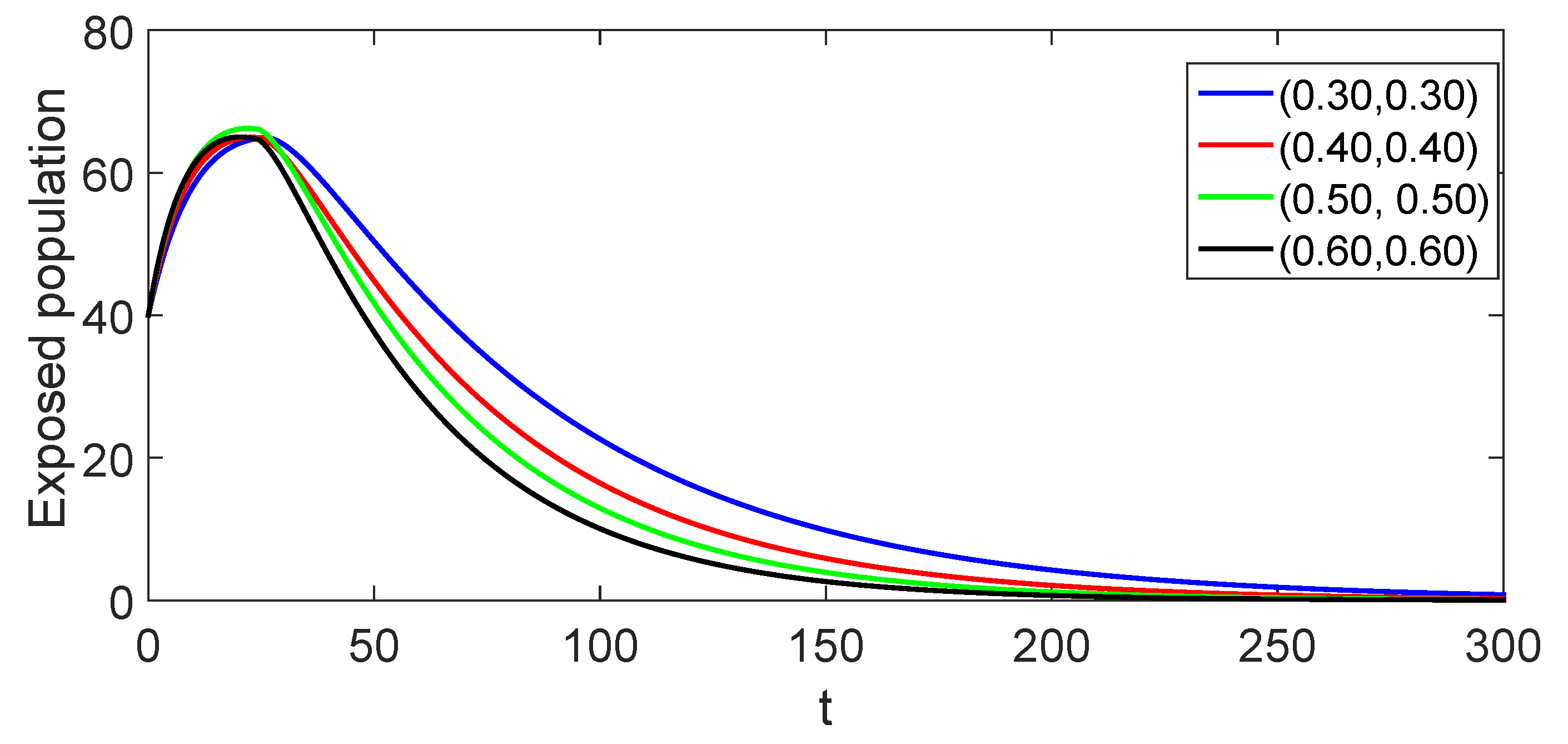
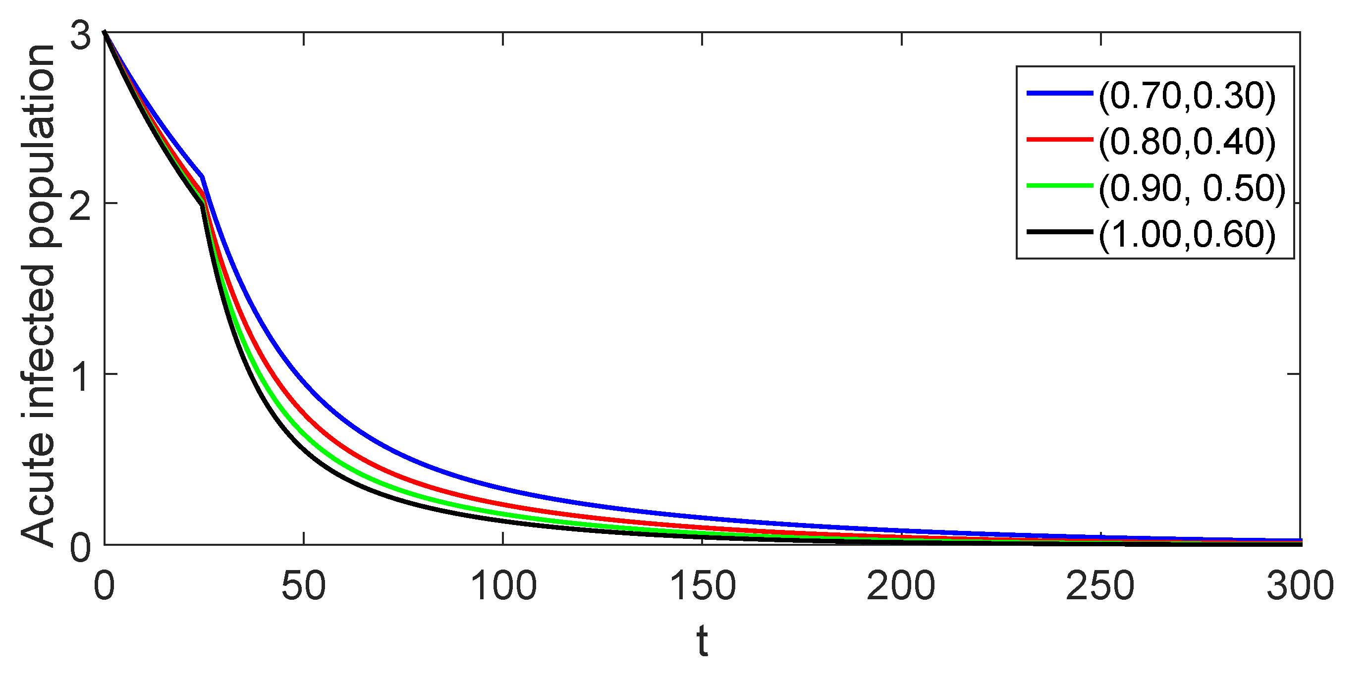
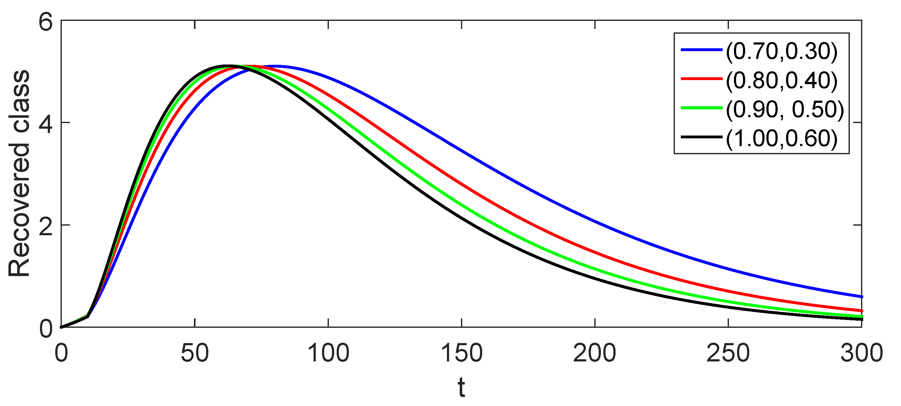
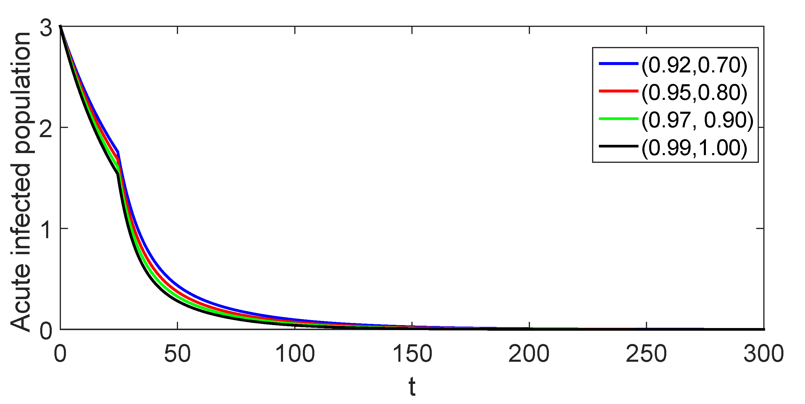
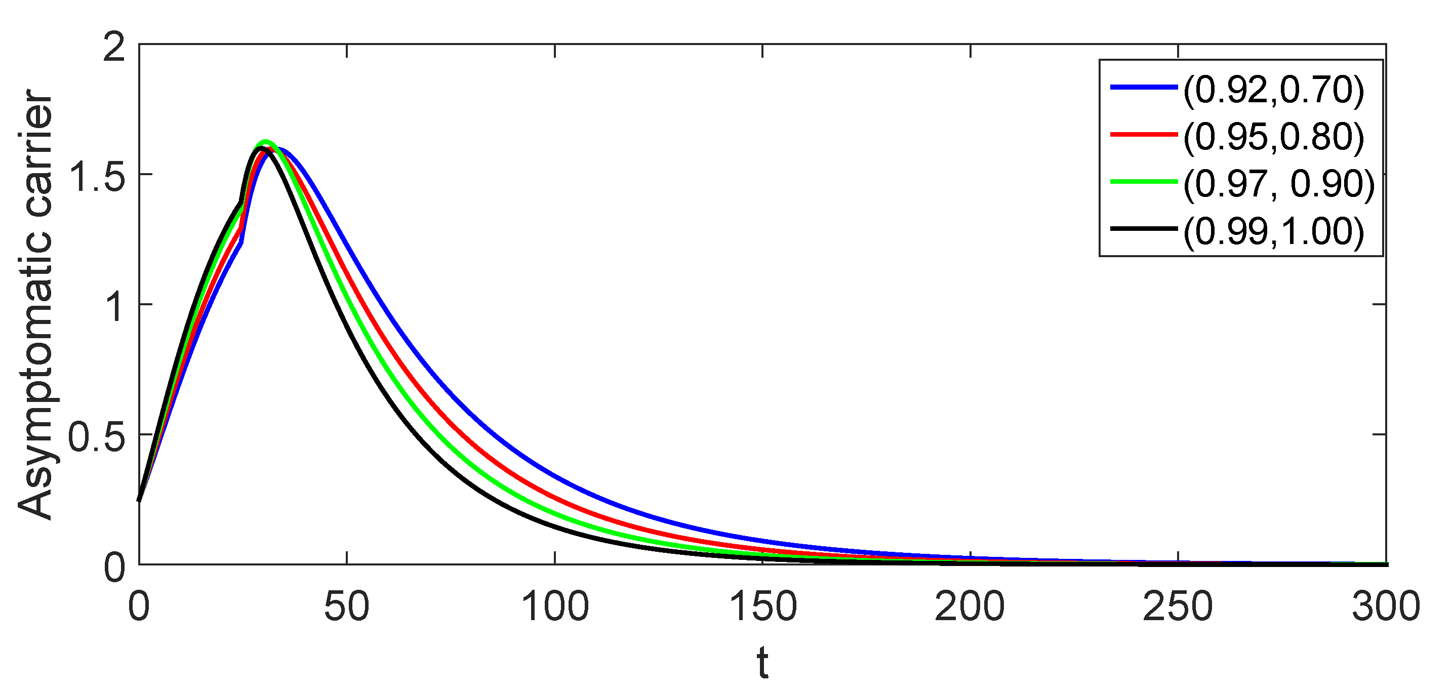
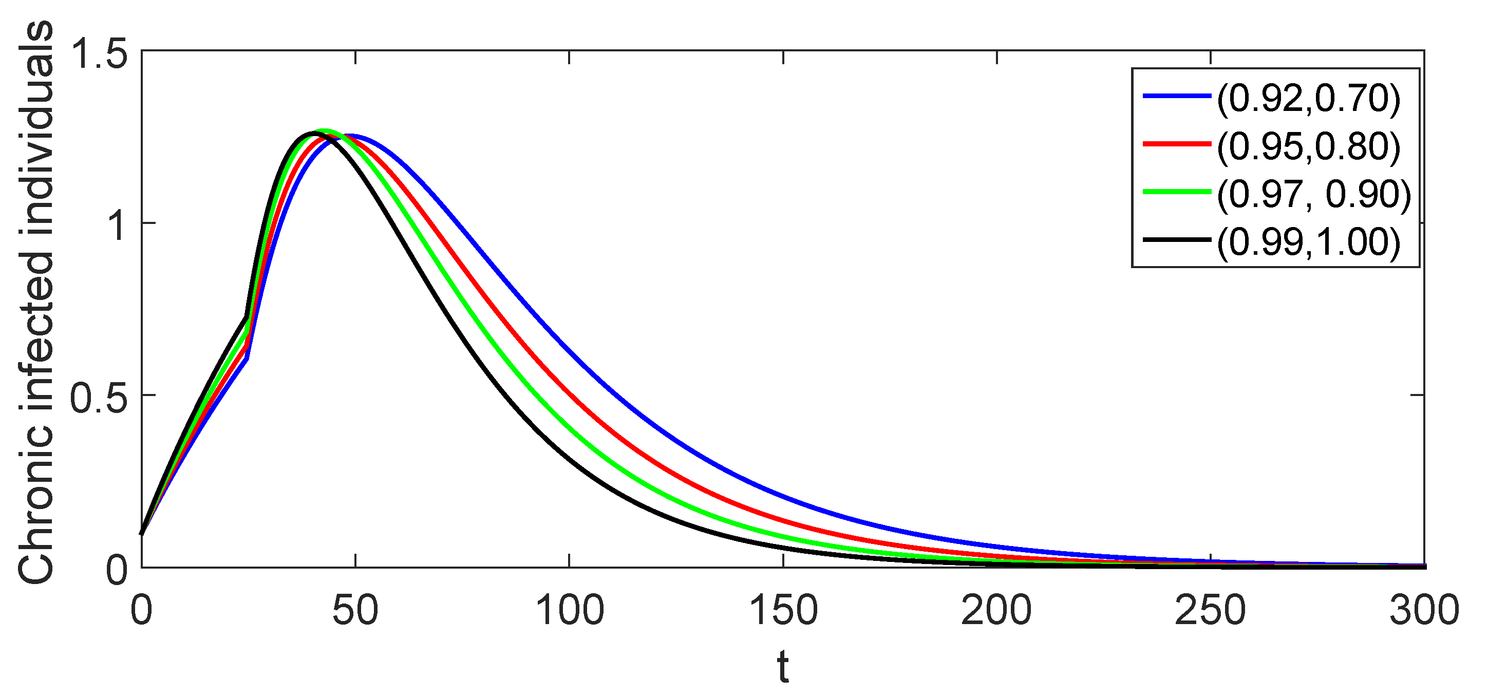
6. Computational Results

From the solution of (10), we have the following integral equation at t = t m + 1 by using (11) with h = t i t i 1
s ( t m + 1 ) = s 0 + η Γ ( ς ) 0 t m + 1 v η 1 ( t m + 1 v ) ς 1 F ( v , s ( v ) ) d v , i f t m + 1 0 , t 1 , s ( t 1 ) + ( 1 ς ) B ( ς ) η t m + 1 η 1 F ( t m + 1 , s ( t m + 1 ) ) ( 1 ς ) B ( ς ) η t m 1 η 1 F ( t m 1 , s ( t m 1 ) ) + ς η B ( ς ) t 1 t m + 1 v η 1 F ( v , s ( v ) ) d v , i f   t t 1 , T .
We can further write (20) as follows:
s ( t m + 1 ) = s 0 + η Γ ( ς ) = 0 m t t + 1 v η 1 ( t + 1 v ) ς 1 F ( v , s ( v ) ) d v , i f t + 1 0 , t 1 , s ( t 1 ) + ( 1 ς ) B ( ς ) η t m + 1 η 1 F ( t m + 1 , s ( t m + 1 ) ) ( 1 ς ) B ( ς ) η t m 1 η 1 F ( t m 1 , s ( t m 1 ) ) + ς η B ( ς ) t 1 t m + 1 v η 1 F ( v , s ( v ) ) d v , i f   t t 1 , T .
We write (21) on using the Lagrange interpolation as follows:
s ( t m + 1 ) = s 0 + η h ς Γ ( ς + 2 ) = 1 m [ t η 1 F ( t , s ( t ) ) ( ( m + 1 ) ς ( m + 2 + ς ) ( m ) ς ( m + 2 + 2 ς ) ) t 1 η 1 F ( t 1 , s ( t 1 ) ) ( ( m + 1 ) ς 1 ( m ) ς ( m + 1 + ς ) ) ] , i f t + 1 0 , t 1 , s ( t 1 ) + ( 1 ς ) B ( ς ) η t m + 1 η 1 F ( t m + 1 , s ( t m + 1 ) ) ( 1 ς ) B ( ς ) η t m 1 η 1 F ( t m 1 , s ( t m 1 ) ) + ς η B ( ς ) [ 3 h t m η 1 2 F ( t m , s ( t m ) ) h t m 1 η 1 2 F ( t m 1 , s ( t m 1 ) ) , i f t t 1 , T ,
which, in the most compact form, can be written as follows:
s ( t m + 1 ) = s 0 + η h ς Γ ( ς + 2 ) = 1 m [ t η 1 F ( t , s ( t ) ) ( ( m + 1 ) ς ( m + 2 + ς ) ( m ) ς ( m + 2 + 2 ς ) ) t 1 η 1 F ( t 1 , s ( t 1 ) ) ( ( m + 1 ) ς 1 ( m ) ς ( m + 1 + ς ) ) ] , i f t + 1 0 , t 1 , s ( t 1 ) + η t m + 1 η 1 [ ( 1 ς ) U ( ς ) + 3 ς h U ( ς ) ] F ( t m , s ( t m ) ) η t m 1 η 1 [ ( 1 ς ) U ( ς ) + ς h U ( ς ) ] F ( t m 1 , s ( t m 1 ) ) , i f t t 1 , T .
To deduce the numerical scheme for the proposed model (6), consider s = X , E , A , A c , C , R p , and we write the right side of the proposed model (6) as follows:
D t ς , η P C F F X ( t ) = Φ 1 ( t , s ( t ) ) , D t ς , η P C F F E ( t ) = Φ 2 ( t , s ( t ) ) , D t ς , η P C F F A ( t ) = Φ 3 ( t , s ( t ) ) , D t ς , η P C F F A c ( t ) = Φ 4 ( t , s ( t ) ) , D t ς , η P C F F C ( t ) = Φ 5 ( t , s ( t ) ) , D t ς , η P C F F R p ( t ) = Φ 6 ( t , s ( t ) ) .
Now, in view of (22), the numerical scheme for system (23) can be written as follows:
X ( t m + 1 ) = X 0 + η h ς Γ ( ς + 2 ) = 1 m [ t η 1 Φ 1 ( t , s ( t ) ) ( ( m + 1 ) ς ( m + 2 + ς ) ( m ) ς ( m + 2 + 2 ς ) ) t 1 η 1 Φ 1 ( t 1 , s ( t 1 ) ) ( ( m + 1 ) ς 1 ( m ) ς ( m + 1 + ς ) ) ] , i f t + 1 0 , t 1 , X ( t 1 ) + η t m + 1 η 1 [ ( 1 ς ) U ( ς ) + 3 ς h U ( ς ) ] Φ 1 ( t m , s ( t m ) ) η t m 1 η 1 [ ( 1 ς ) U ( ς ) + ς h U ( ς ) ] Φ 1 ( t m 1 , s ( t m 1 ) ) , i f t t 1 , T ,
E ( t m + 1 ) = E 0 + η h ς Γ ( ς + 2 ) = 1 m [ t η 1 Φ 2 ( t , s ( t ) ) ( ( m + 1 ) ς ( m + 2 + ς ) ( m ) ς ( m + 2 + 2 ς ) ) t 1 η 1 Φ 2 ( t 1 , s ( t 1 ) ) ( ( m + 1 ) ς 1 ( m ) ς ( m + 1 + ς ) ) ] , i f t + 1 0 , t 1 , E ( t 1 ) + η t m + 1 η 1 [ ( 1 ς ) U ( ς ) + 3 ς h U ( ς ) ] Φ 2 ( t m , s ( t m ) ) η t m 1 η 1 [ ( 1 ς ) U ( ς ) + ς h U ( ς ) ] Φ 2 ( t m 1 , s ( t m 1 ) ) , i f t t 1 , T ,
A ( t m + 1 ) = A 0 + η h ς Γ ( ς + 2 ) = 1 m [ t η 1 Φ 3 ( t , s ( t ) ) ( ( m + 1 ) ς ( m + 2 + ς ) ( m ) ς ( m + 2 + 2 ς ) ) t 1 η 1 Φ 3 ( t 1 , s ( t 1 ) ) ( ( m + 1 ) ς 1 ( m ) ς ( m + 1 + ς ) ) ] , i f t + 1 0 , t 1 , A ( t 1 ) + η t m + 1 η 1 [ ( 1 ς ) U ( ς ) + 3 ς h U ( ς ) ] Φ 3 ( t m , s ( t m ) ) η t m 1 η 1 [ ( 1 ς ) U ( ς ) + ς h U ( ς ) ] Φ 3 ( t m 1 , s ( t m 1 ) ) , i f t t 1 , T ,
A c ( t m + 1 ) = A c , 0 + η h ς Γ ( ς + 2 ) = 1 m [ t η 1 Φ 4 ( t , s ( t ) ) ( ( m + 1 ) ς ( m + 2 + ς ) ( m ) ς ( m + 2 + 2 ς ) ) t 1 η 1 Φ 4 ( t 1 , s ( t 1 ) ) ( ( m + 1 ) ς 1 ( m ) ς ( m + 1 + ς ) ) ] , i f t + 1 0 , t 1 , A c ( t 1 ) + η t m + 1 η 1 [ ( 1 ς ) U ( ς ) + 3 ς h U ( ς ) ] Φ 4 ( t m , s ( t m ) ) η t m 1 η 1 [ ( 1 ς ) U ( ς ) + ς h U ( ς ) ] Φ 4 ( t m 1 , s ( t m 1 ) ) , i f t t 1 , T ,
C ( t m + 1 ) = C 0 + η h ς Γ ( ς + 2 ) = 1 m [ t η 1 Φ 5 ( t , s ( t ) ) ( ( m + 1 ) ς ( m + 2 + ς ) ( m ) ς ( m + 2 + 2 ς ) ) t 1 η 1 Φ 5 ( t 1 , s ( t 1 ) ) ( ( m + 1 ) ς 1 ( m ) ς ( m + 1 + ς ) ) ] , i f t + 1 0 , t 1 , C ( t 1 ) + η t m + 1 η 1 [ ( 1 ς ) U ( ς ) + 3 ς h U ( ς ) ] Φ 5 ( t m , s ( t m ) ) η t m 1 η 1 [ ( 1 ς ) U ( ς ) + ς h U ( ς ) ] Φ 5 ( t m 1 , s ( t m 1 ) ) , i f t t 1 , T ,
and
R p ( t m + 1 ) = R p , 0 + η h ς Γ ( ς + 2 ) = 1 m [ t η 1 Φ 6 ( t , s ( t ) ) ( ( m + 1 ) ς ( m + 2 + ς ) ( m ) ς ( m + 2 + 2 ς ) ) t 1 η 1 Φ 6 ( t 1 , s ( t 1 ) ) ( ( m + 1 ) ς 1 ( m ) ς ( m + 1 + ς ) ) ] , i f t + 1 0 , t 1 , R p ( t 1 ) + η t m + 1 η 1 [ ( 1 ς ) U ( ς ) + 3 ς h U ( ς ) ] Φ 6 ( t m , s ( t m ) ) η t m 1 η 1 [ ( 1 ς ) U ( ς ) + ς h U ( ς ) ] Φ 6 ( t m 1 , s ( t m 1 ) ) , i f t t 1 , T .

Simulations and Explanation

In view of the numerical scheme given above, we simulate our results by taking the parameter values as used by [20] in the numerical analysis: ϱ = 2 , ξ = 1 67.7 , ϑ = 0.042 , ω 1 = 1 = 0.002 , ψ 1 = 0.004 , n = 0.6 , μ = 0.001 , ρ 1 = η 1 = x 1 = 0.02 , λ = 0.1 , δ = 0.003 , z 1 = 0.01 , and v 1 = 0.2 . Also, the initial data are taken as follows:
X 0 , E 0 , A 0 , A c , C 0 , R p 0 = ( 60 , 40 , 3 , 0.25 , 0.1 , 0 ) .
Consider three sets of fractal–fractional orders as X 1 = [ 0 , 0.60 ] , X 2 = [ 0.60 , 0.95 ] , X 3 = [ 0.90 , 1.0 ] . Different graphical presentations are given here to simulate our results. First, we consider the fractal–fractional order values in the first set X 1 , as presented in Figure 1, Figure 2, Figure 3, Figure 4, Figure 5 and Figure 6.
In addition, we present the results for another set of fractal–fractional orders in Figure 7, Figure 8, Figure 9, Figure 10 and Figure 11, respectively.
In addition, we graphically present the results for another set of fractal–fractional orders in Figure 12, Figure 13, Figure 14, Figure 15, Figure 16 and Figure 17, respectively.
We used various fractal–fractional order values to interpret the results graphically in Figure 1, Figure 2, Figure 3, Figure 4, Figure 5, Figure 6, Figure 7, Figure 8, Figure 9, Figure 10, Figure 11, Figure 12, Figure 13, Figure 14, Figure 15, Figure 16 and Figure 17, respectively. From the numerical presentation, we observe the crossover behaviors of each compartment near the point t 1 = 50 . The corresponding decline in the affected class is shown in Figure 1 and Figure 12 for different fractal–fractional orders. The exposed class initially grows but then declines, which is different at different values of fractal–fractional orders. The aforementioned dynamics for the exposed class are shown in Figure 2, Figure 7, and Figure 13, respectively. From Figure 3, Figure 8, and Figure 14, we observe a decline in the population with a crossover effect near the point t 1 = 50 using different fractal–fractional order values. Also, the class of asymptomatic carriers is presented graphically using different fractal–fractional order values in Figure 4, Figure 9, and Figure 15, respectively, for numerous values of fractal–fractional orders. This class exhibits growth for the first 50 days and then shows a decline. The population of the model classes, representing exposed, asymptomatic carriers, and chronically infected individuals, grows and peaks at t 1 = 25 ; however, it begins to decline in the second sub-interval. These graphical presentations clearly demonstrate the crossover behavior in each class near the point t 1 = 25 . The class of chronically infected individuals shows growth for the first 100 days and then starts to decline, as depicted in Figure 5, Figure 10, and Figure 16. The recovered class shows growth for the initial 100 days, as presented in Figure 6, Figure 11, and Figure 17, respectively, for different values of fractal–fractional orders.

7. Conclusions

In this research work, we conducted a detailed and comprehensive analysis of the Hepatitis B mathematical model using piecewise fractal–fractional analysis. We introduced piecewise fractal–fractional differential operators, which have not previously been considered in the literature. While the available literature contains many results on various piecewise fractional derivatives, models with piecewise fractal-fractional derivatives are rarely studied. We considered our piecewise derivative in a different pattern than the previous concept of piecewise derivatives and integrals. We divided the time interval into two subintervals. In the first one, we considered an FFD with a power law kernel, and in the second one, we considered an FFD with an exponential decay kernel. The disease-free equilibrium point of the proposed model was presented as well. In the main results, we examined the existence and stability of the proposed model. For the numerical results of the model and visual presentation, we used the Lagrange interpolation method and extended the ABM method, respectively. Upon using the said numerical scheme, we presented our results for different values of fractal–fractional orders. Also, we presented results for three different sets of fractal–fractional order values. The concerned dynamics with the crossover effect were presented graphically for each component of the proposed model. In the future, the piecewise fractal–fractional concept could be extended to other dynamical problems.

Author Contributions

Conceptualization, Z.A.K. and A.A.; Methodology, Z.A.K.; Validation, A.U.R.I.; Formal analysis, A.U.R.I.; Investigation, B.O.; Data curation, B.O.; Writing—original draft, A.A.; Writing—review & editing, H.A. All authors have read and agreed to the published version of the manuscript.

Funding

This research was funded by Princess Nourah bint Abdulrahman University grant number PNURSP2024R8.

Data Availability Statement

Data are contained within the article.

Acknowledgments

Princess Nourah bint Abdulrahman University Researchers supporting project number (PNURSP2024R8). Princess Nourah bint Abdulrahman University, Riyadh, Saudi Arabia. A.U. Rehman Irshad and B. Ozdemir are thankful to Prince Sultan University for APC and support through the TAS research lab.

Conflicts of Interest

The authors declare no conflicts of interest.

References

  1. Volterra, V. Théorie mathématique de la lutte pour la vie; Gauthier-Villars: Paris, France, 1931. [Google Scholar]
  2. Lotka, A.J. Elements of Physical Biology; Williams & Wilkins: Baltimore, MD, USA, 1925. [Google Scholar]
  3. Kolmogoroff, A.N. Sulla theoria di Volterra della lotta per l’esistenza. G. Ist. Ital. Attuari 1936, 7, 74–80. [Google Scholar]
  4. Kostitzin, V.A. Mathematical Biology; Harrap: Bromley, UK, 1939. [Google Scholar]
  5. Smith, M. Models in Ecology; Cambridge University Press: Cambridge, UK, 1974. [Google Scholar]
  6. Murray, J. Mathematical Biology; Springer: Berlin, Germany, 1989. [Google Scholar]
  7. Svirezhev, Y.M. Nonlinearities in mathematical ecology: Phenomena and models, would we live in Volterra’s world. Ecol. Model. 2008, 216, 89–101. [Google Scholar] [CrossRef]
  8. Kilbas, A.A.; Shrivastava, H.M.; Trujillo, J.J. Theory and Applications of Fractional Differential Equations; Elsevier: Amsterdam, The Netherlands, 2006. [Google Scholar]
  9. Podlubny, I. Fractional Differential Equations; Academic Press: San Diego, CA, USA, 1999. [Google Scholar]
  10. Caputo, M.; Fabrizio, M. A new definition of fractional derivative without singular kernel. Prog. Fract. Differ. Appl. 2015, 1, 73–85. [Google Scholar]
  11. Losada, J.; Nieto, J.J. Properties of a new fractional derivative without singular kernel. Prog. Fract. Differ. Appl. 2015, 1, 87–92. [Google Scholar]
  12. Atangana, A.; Baleanu, D. New fractional derivative with non-local and non-singular kernel. Therm. Sci. 2016, 20, 757–763. [Google Scholar] [CrossRef]
  13. Atangana, A.; Araz, S.İ. New concept in calculus: Piecewise differential and integral operators. Chaos Solitons Fractals 2021, 145, 110638. [Google Scholar] [CrossRef]
  14. Atangana, A.; Araz, S.I. Piecewise derivatives versus short memory concept: Analysis and application. AIMs Math. 2022, 19, 8601–8620. [Google Scholar]
  15. Atangana, A. Fractal-fractional differentiation and integration: Connecting fractal calculus and fractional calculus to predict complex system. Chaos Solitons Fractals 2017, 102, 396–406. [Google Scholar] [CrossRef]
  16. Shah, K.; Abdeljawad, T. Study of radioactive decay process of uranium atoms via fractals-fractional analysis. S. Afr. J. Chem. Eng. 2024, 48, 63–70. [Google Scholar] [CrossRef]
  17. Khan, H.; Aslam, M.; Rajpar, A.H.; Chu, Y.M.; Etemad, S.; Rezapour, S.; Ahmad, H. A new fractal-fractional hybrid model for studying climate change on coastal ecosystems from the mathematical point of view. Fractals 2024, 32, 2440015. [Google Scholar] [CrossRef]
  18. Khan, H.; Alzabut, J.; Shah, A.; He, Z.Y.; Etemad, S.; Rezapour, S.; Zada, A. On fractal-fractional waterborne disease model: A study on theoretical and numerical aspects of solutions via simulations. Fractals 2023, 31, 2340055. [Google Scholar] [CrossRef]
  19. Shah, A.; Khan, H.; De la Sen, M.; Alzabut, J.; Etemad, S.; Deressa, C.T.; Rezapour, S. On non-symmetric fractal-fractional modeling for ice smoking: Mathematical analysis of solutions. Symmetry 2022, 15, 87. [Google Scholar] [CrossRef]
  20. Gul, N.; Bilal, R.; Algehyne, E.A.; Alshehri, M.G.; Khan, M.A.; Chu, Y.M.; Islam, S. The dynamics of fractional order Hepatitis B virus model with asymptomatic carriers. Alex. Eng. J. 2021, 60, 3945–3955. [Google Scholar] [CrossRef]
  21. Aldwoah, K.A.; Almalahi, M.A.; Shah, K. Theoretical and Numerical Simulations on the Hepatitis B Virus Model through a Piecewise Fractional Order. Fractal Fract. 2023, 7, 844. [Google Scholar] [CrossRef]
  22. Van den Driessche, P.; Watmough, J. Reproduction numbers and sub-threshold endemic equilibria for compartmental models of disease transmission. Math. Biosci. 2002, 180, 29–48. [Google Scholar] [CrossRef] [PubMed]
Figure 1. Numerical interpretation of various values of fractal–fractional orders in the set X 1 for the affected class.
Fractalfract 08 00260 g001
Figure 2. Numerical interpretation of various values of fractal–fractional orders in the set X 1 for the exposed class.
Fractalfract 08 00260 g002
Figure 3. Numerical interpretation of various values of fractal–fractional orders in the set X 1 for the acutely infected class.
Fractalfract 08 00260 g003
Figure 4. Numerical interpretation of various values of fractal–fractional orders in the set X 1 for the asymptomatic carrier class.
Fractalfract 08 00260 g004
Figure 5. Numerical interpretation of various values of fractal–fractional orders in the set X 1 for chronically infected individuals.
Fractalfract 08 00260 g005
Figure 6. Numerical interpretation of various values of fractal–fractional orders in the set X 1 for recovered individuals.
Fractalfract 08 00260 g006
Figure 7. Numerical interpretation of various values of fractal–fractional orders in the set X 1 for the exposed class.
Fractalfract 08 00260 g007
Figure 8. Numerical interpretation of various values of fractal–fractional orders in the set X 2 for the acutely infected class.
Fractalfract 08 00260 g008
Figure 9. Numerical interpretation of various values of fractal–fractional orders in the set X 2 for the asymptomatic carrier class.
Fractalfract 08 00260 g009
Figure 10. Numerical interpretation of various values of fractal–fractional orders in the set X 2 for chronically infected individuals.
Fractalfract 08 00260 g010
Figure 11. Numerical interpretation of various values of fractal–fractional orders in the set X 2 for recovered individuals.
Fractalfract 08 00260 g011
Figure 12. Numerical interpretation of various values of fractal–fractional orders in the set X 3 for the affected class.
Fractalfract 08 00260 g012
Figure 13. Numerical interpretation of various values of fractal–fractional orders in the set X 3 for the exposed class.
Fractalfract 08 00260 g013
Figure 14. Numerical interpretation of various values of fractal–fractional orders in the set X 3 for the acutely infected class.
Fractalfract 08 00260 g014
Figure 15. Numerical interpretation of various values of fractal–fractional orders in the set X 3 for the asymptomatic carrier class.
Fractalfract 08 00260 g015
Figure 16. Numerical interpretation of various values of fractal–fractional orders in the set X 3 for chronically infected individuals.
Fractalfract 08 00260 g016
Figure 17. Numerical interpretation of various values of fractal–fractional orders in the set X 3 for recovered individuals.
Fractalfract 08 00260 g017
Table 1. Parameters for system (6).
ParametersParameter Definition
X ( t ) Susceptible class of individuals.
E ( t ) Exposed class of population.
A ( t ) Acute class of infected individuals.
A c ( t ) Asymptomatic carrier.
C ( t ) Chronic class of infected individuals.
R p ( t ) Recovered class of individuals.
Disclaimer/Publisher’s Note: The statements, opinions and data contained in all publications are solely those of the individual author(s) and contributor(s) and not of MDPI and/or the editor(s). MDPI and/or the editor(s) disclaim responsibility for any injury to people or property resulting from any ideas, methods, instructions or products referred to in the content.

