Investigation of a Spatio-Temporal Fractal Fractional Coupled Hirota System

Abstract

This article aims to examine the nonlinear excitations in a coupled Hirota system described by the fractal fractional order derivative. By using the Laplace transform with Adomian decomposition (LADM), the numerical solution for the considered system is derived. It has been shown that the suggested technique offers a systematic and effective method to solve complex nonlinear systems. Employing the Banach contraction theorem, it is confirmed that the LADM leads to a convergent solution. The numerical analysis of the solutions demonstrates the confinement of the carrier wave and the presence of confined wave packets. The dispersion nonlinear parameter reduction equally influences the wave amplitude and spatial width. The localized internal oscillations in the solitary waves decreased the wave collapsing effect at comparatively small dispersion. Furthermore, it is also shown that the amplitude of the solitary wave solution increases by reducing the fractal derivative. It is evident that decreasing the order $\alpha$ modifies the nature of the solitary wave solutions and marginally decreases the amplitude. The numerical and approximation solutions correspond effectively for specific values of time (t). However, when the fractal or fractional derivative is set to one by increasing time, the wave amplitude increases. The absolute error analysis between the obtained series solutions and the accurate solutions are also presented.

1. Introduction

In recent decades, due to the broad applications of soliton theory in physics, mathematics, and other areas of engineering and applied sciences, the analysis of explicit accurate solutions in the form of solitary wave solutions of evolution equations has played a significant role [1,2,3]. In soliton theory, several analytical methods can be applied to calculate the approximate solution to nonlinear partial differential equations [4,5,6]. To investigate fractal fractional nonlinear coupled Hirota systems, we consider the Hirota equation [7]

$$\begin{array}{c}\hfill \frac{\partial \psi (x,t)}{\partial t}+{3\delta \left|\psi (x,t)\right|}^2\frac{\partial \psi (x,t)}{\partial x}+\gamma \frac{{\partial }^3\psi (x,t)}{\partial x^3}=0,t>0,x\in [-\infty ,\infty ],\end{array}$$

(1)

where the function $\psi (x,t)$ is a complex-valued function, and $\delta ,\gamma \in {\mathbb{R}}^{+}$. The Hirota equation is a modified nonlinear Schrödinger equation (NLSE) that considers higher-order dispersion and time-delay corrections to the cubic nonlinearity [8]. It can be observed as a generalization for the NLS equation when the higher dispersion and time-delay changes are considered, as well as complex generalization of the mKdV equation [9]. It is also known as soliton equation because this usually has an exact solution where localized moving excitations that preserve their shape in the evolution, similarly to the NLS soliton [10,11]. The Hirota equation was initially studied to illustrate the ultra-short pulses experienced from the self-steepening effect and high-order dispersion [8]. It has numerous applications, such as localized wave structures, transmission of optical pulses in optical waveguide arrays, rogue waves, solitary waves, and breathers [12,13]. It has also been widely studied for rational solitary and rogue wave solutions, interaction properties of complex modified solitons, multi-solitons, dark-bright-rogue wave phenomena, and rogue wave pairs [14,15,16,17]. The Hirota equation has been analytically investigated using different methods containing the Hamiltonian formalism, perturbation theory, Darboux transformation, sine–cosine, and tangent methods [18,19,20,21]. The Hirota Equation (1) possess more than one parameter solutions in the form solitons, analogous to NLS equation subjected to velocity and amplitude as

$$\begin{array}{ccc}\hfill \psi (x,t)& =& Asech\left[\eta (x-\mu t)\right]e^{ik\left(x-\omega t\right)},\hfill \end{array}$$

(2)

where $A=k\sqrt{2\gamma /\delta }$ is the amplitude and $\mu =\gamma ({\eta }^2-3k^2)$ represents the wave speed. The frequency of the phase is given by $\omega =\gamma (3{\eta }^2-k^2)$, where $\gamma$ represents nonlinearity dispersion coefficients, $\eta$ is the wave envelope’s width, and k is the propagation number. By using assumption $\psi =\varphi (x,t)+i\phi (x,t)$, the Hirota equation can be transformed to coupled Hirota system [22,23]

$$\begin{array}{c}\hfill \frac{\partial \varphi }{\partial t}+3\delta \left({\varphi }^2+{\phi }^2\right)\frac{\partial \varphi }{\partial x}+\gamma \frac{{\partial }^3\varphi }{\partial x^3}=0,\end{array}$$

(3)

$$\begin{array}{c}\hfill \frac{\partial \phi }{\partial t}+3\delta \left({\varphi }^2+{\phi }^2\right)\frac{\partial \phi }{\partial x}+\gamma \frac{{\partial }^3\phi }{\partial x^3}=0.\end{array}$$

(4)

It should be noted that converting the Hirota equation to a coupled Hirota system allows for the study of growth or decay in the system (the real and imaginary parts of the function $\psi (x,t)$) separately, leading to deeper insights into the solitary wave solutions. Similar to Equation (1), the coupled Hirota system has also been investigated to describe propagation of electromagnetic pulses in optical fibres by employing the inverse scattering transform [24]. Several other interesting results have been examined for coupled Hirota system, such as relation amongst dark–bright solitons, Lax pair, Painlevé analyses and rogue waves solutions [25,26,27]. Here, we use the concept of fractional fractal derivative of order $(\alpha ,\beta )$ to study the coupled Hirota system

$$\begin{array}{c}\hfill {}^{FFP}D_t^{\alpha ,\beta }\varphi +3\delta \left({\varphi }^2+{\phi }^2\right)\frac{\partial \varphi }{\partial x}+\gamma \frac{{\partial }^3\varphi }{\partial x^3}=0,\end{array}$$

(5)

$$\begin{array}{c}\hfill {}^{FFP}D_t^{\alpha ,\beta }\phi +3\delta \left({\varphi }^2+{\phi }^2\right)\frac{\partial \phi }{\partial x}+\gamma \frac{{\partial }^3\phi }{\partial x^3}=0,\end{array}$$

(6)

where the classical time partial derivatives are replaced with fractional derivatives of the functions of order $\alpha$ ($0<\alpha \le 1$) in the Caputo sense with power law kernel and fractal derivative $\beta$ ($0<\beta \le 1$). The initial conditions considered herein are

$$\begin{array}{c}\hfill \varphi (x,0)=f\left(x\right),\phi (x,0)=g\left(x\right).\end{array}$$

(7)

The concept of fractional calculus (FC) originated from the challenge that even the concept of a derivative of a classical order could potentially be expanded to stay authentic when the order was not an integer. Following this exceptional theory, the subject of FC caught great attention in mathematics and other areas of scientific research. Since then, FC has been extensively used to examine various physical facts, such as electromagnetic, viscoelastic, and damping theories, artificial intelligence, fluid dynamics, wave propagation theories, chaotic dynamics, heat transfer analysis, appliances, control systems, and various inherent algorithms [28,29,30,31,32,33,34].

In FC, the classical integrals and derivatives are expanded to fractional order as the standard operators are inadequate for understanding many complex systems, because fractional operators produce more realistic and precise results. Numerous fractional derivatives have been derived with distinct kinds of kernels, such as Hilfer, Riemann–Liouville (RL), Caputo, Grünwald, Caputo–Fabrizio, and Atangana–Baleanu derivatives [35,36]. Similarly, several novel kinds of fractional operators have proposed to link the ideas of Caputo and other fractional operators [37,38].

In addition to the fractional-order operators, another new theory of differentiation has been suggested, where the derivative is represented as the fractional order with fractal dimension [39]. The fundamental concept is called fractal fractional integrals and derivatives [40]. If the system under investigation is derivable, the fractal derivative becomes $\beta t^{\beta -1}$, and the classical operator is regained when the fractal order reaches one [41]. In a fractal derivative, the variable is ascended, corresponding to $t^{\alpha }$. This modified derivative was proposed to model certain real-world physical systems for which conventional physical phenomena are not appropriate and cannot be applied to the non-integral means of fractal dimension [42,43]. The theory of fractal fractional integrals and derivatives has been extensively used in engineering applications (fluid motion, aquifer, and crystallization), chaotic processes, and electronic networks [44,45]. Here, we will investigate the localized excitations in a coupled Hirota system with time fractional derive in Caputo’s sense with fractal dimension. The Laplace transform with Adomian decomposition is a very effective analytical technique, and has been successfully applied to investigate numerous mathematical problems in classical as well as in fractional calculus. We will derive the series solution of the considered system in a systematic manner using LADM.

The article is organized as follows: In Section 2, various fundamental definitions of fractional calculus are included. In Section 3, the general series solution of the coupled Hirota system with order $(\alpha ,\beta )$ is calculated using LADM. The convergence analysis of LADM is examined in Section 4. For confirmation of the obtained findings, a particular example is studied in Section 5 with absolute error analysis. The systematic approximate solutions are compared with numerical results with comprehensive discussions in Section 6.

2. Preliminaries

Here, we state fundamental definitions associated with fractal fractional calculus and the Laplace and inverse Laplace transforms that will be applied in the next section.

Definition 1. 

Let $\psi \in H^1$, and $\alpha \in (0,1]$; we define the Caputo’s derivative as

$$\begin{array}{c}\hfill {}_a{}^{C}D_t^{\alpha }\psi \left(t\right)={}_{a}I_t^{(n-\alpha )}\left[\frac{d^n}{d{t}^n}\psi \left(t\right)\right]=\frac{1}{\mathrm{\Gamma }(p-\alpha )}{\int }_a^t{(t-s)}^{p-\alpha -1}{\psi }^{\prime }\left(s\right)ds,p-1<\alpha \le p.\end{array}$$

Definition 2. 

Let $\psi \left(t\right)$ be an open differentiable interval $(a,b)$. If $\psi \left(t\right)$ is fractal fractional differentiable on $(a,b)$, with fractal order β, then the fractal fractional derivative of order α in Caputo sense with power law kernel is given by [40]

$$\begin{array}{c}\hfill {}_a{}^{FFP}D_t^{\alpha ,\beta }\psi \left(t\right)=\frac{1}{\mathrm{\Gamma }(p-\alpha )}{\int }_a^t{(t-s)}^{p-\alpha -1}\frac{d}{d{s}^{\beta }}\psi \left(s\right)ds,<p-1<\alpha \le p,<p-1<\beta \le p,\end{array}$$

where $\frac{d\psi \left(s\right)}{d{s}^{\beta }}={lim}_{t\to s}\frac{\psi \left(t\right)-\psi \left(s\right)}{t^{\beta }-s^{\beta }}$. The above operator can also be represented as

$$\begin{array}{c}\hfill {}_a{}^{FFP}D_t^{\alpha ,\beta }\psi \left(t\right)=\frac{1}{\mathrm{\Gamma }(p-\alpha )}{\int }_a^t{(t-s)}^{p-\alpha -1}\frac{d^{\gamma }}{d{s}^{\beta }}\psi \left(s\right)ds,p-1<\alpha ,\beta ,\le p,\end{array}$$

where $\frac{d^{\gamma }\psi \left(s\right)}{d{s}^{\beta }}={lim}_{t\to s}\frac{{\psi }^{\gamma }\left(t\right)-{\psi }^{\gamma }\left(s\right)}{t^{\beta }-s^{\beta }}$.

Definition 3. 

Let $\psi \left(t\right)$ be a continuous function on the interval I, then the fractional integral of $\psi \left(t\right)$ with fractional order α can be described [40]

$$\begin{array}{ccc}\hfill {}_a{}^F\mathbb{I}_t^{\alpha }\psi \left(t\right)& =& \alpha {\int }_0^t{s}^{\alpha -1}\psi \left(s\right)ds.\hfill \end{array}$$

From the above, the fractal fractional integral can be obtained as [40]

$$\begin{array}{ccc}\hfill {}_t{}^{FFP}\mathbb{I}_t^{\alpha }\psi \left(t\right)& =& \frac{\beta }{(\alpha -1)!}{\int }_0^t{s}^{\alpha -1}{(t-s)}^{\alpha -1}\psi \left(s\right)ds.\hfill \end{array}$$

Definition 4. 

For a function $\psi \left(t\right)$, the Laplace transform is symbolized by $\mathbb{L}$ and is defined as [46]

$$\begin{array}{c}\hfill \mathbb{L}\left[\psi \left(t\right)\right]=\mathbb{F}\left(s\right)={\int }_0^{\infty }{e}^{-st}\psi \left(s\right)ds,t>0.\end{array}$$

Definition 5. 

If $\psi \left(t\right)={\mathbb{L}}^{-1}\mathbb{F}\left(s\right)$, then the inverse Laplace transform ${\mathbb{L}}^{-1}$ is defined as [46]

$$\begin{array}{c}\hfill {\mathbb{L}}^{-1}\left(\frac{\mathbb{F}\left(s\right)}{s}\right)={\int }_0^t\psi \left(t\right)dt.\end{array}$$

Let $\psi \left(t\right)$ be a continuous function; the fractal Laplace transform of order α can be written as [40]

$$\begin{array}{ccc}\hfill {}^F\mathbb{L}_a^{\alpha }\psi \left(t\right)& =& {\int }_0^{\infty }{t}^{\alpha -1}{e}^{-at}\psi \left(t\right)dt.\hfill \end{array}$$

Definition 6. 

For the function $\psi (x,t)$, applying Laplace transform to Caputo fractional derivative, we obtain

$$\begin{array}{c}\hfill {\mathbb{L}}_a^C{D}_t^{\alpha }\psi (x,t)=s^{\alpha }\mathbb{L}\psi (x,t)-\sum _{k=0}^{n-1}{s}^{\alpha -k-1}{\psi }_{kt}(x,0),n=\left[\alpha \right]+1.\end{array}$$

3. General Solution of Fractal Fractional Coupled Hirota System

Here, we discuss properties of Laplace transform with order $(\alpha ,\beta )$ and calculate coupled the Hirota system with fractal fractional derivative of order $\alpha$ using the Laplace Adomian decomposition method. In 1980, George Adomian established a novel approach to solving nonlinear functional equations. Since then, this technique has been called the Adomian decomposition method (ADM), and has been applied in numerous studies [47,48]. The ADM involves breaking down the equation under consideration into linear and nonlinear parts and generates the series solution, whose terms are determined by a recursive relation using the Adomian polynomials. Numerous fundamental studies on various aspects of the extended version of Adomian’s decomposition method have been performed [49,50,51]. Similarly, the extended version of the Laplace decomposition method has been used for the solution of different PDEs [52].

Suppose $\psi \left(t\right)\in H^1$ is a continuous function ∀$t\in [0,T]$, such that

$$\begin{array}{c}\hfill {}^{FFP}D_t^{\alpha ,\beta }\psi \left(t\right)=F\left(x\right).\end{array}$$

(8)

Using the definition presented in [45], we can write

$$\begin{array}{c}\hfill {}^{C}D_t^{\alpha }\psi \left(t\right)=\beta t^{\beta -1}F\left(x\right).\end{array}$$

(9)

Implementing the Laplace transformation to Equation (9) yields

$$\begin{array}{ccc}\hfill \mathbb{L}\left[\psi \right(t\left)\right]& =& \frac{\psi \left(0\right)}{s}+\frac{1}{s^{\alpha }}\mathbb{L}\left[\beta t^{\beta -1}F\left(x\right)\right],\hfill \\ \hfill \psi \left(t\right)& =& {\mathbb{L}}^{-1}\left[\frac{\psi \left(0\right)}{s}+\frac{1}{s^{\alpha }}\mathbb{L}\left(\beta t^{\beta -1}F\left(x\right)\right)\right],\mathrm{applying}{\mathbb{L}}^{-1}\hfill \\ \hfill \psi \left(t\right)& =& \psi \left(0\right)+{\mathbb{L}}^{-1}\left[\frac{\mathrm{\Gamma }(\beta +1)}{s^{\alpha +\beta }}\right]F\left(x\right)=\psi \left(0\right)+\frac{\mathrm{\Gamma }(\beta +1)t^{\alpha +\beta -1}}{\mathrm{\Gamma }(\alpha +\beta )}F\left(x\right).\hfill \end{array}$$

(10)

This is the Laplace transformation of fractal fractional derivative with power law kernel.

To obtain the general solution of system (5) and (6), one can apply definition of fractal derivative, which gives

$$\begin{array}{ccc}\hfill {}^{C}D_t^{\alpha }\varphi & =& \beta t^{\beta -1}\left[-3\delta {\varphi }^2{\varphi }_x-3\delta {\phi }^2{\varphi }_x-\gamma {\varphi }_{xxx}\right],\hfill \end{array}$$

(11)

$$\begin{array}{ccc}\hfill {}^{C}D_t^{\alpha }\phi & =& \beta t^{\beta -1}\left[-3\delta {\varphi }^2{\phi }_x-3\delta {\phi }^2{\phi }_x-\gamma {\phi }_{xxx}\right].\hfill \end{array}$$

(12)

Applying the Laplace transformation

$$\begin{array}{ccc}\hfill \mathbb{L}{[}^C{D}_t^{\alpha }\varphi ]& =& \mathbb{L}\left[\beta t^{\beta -1}(-3\delta {\varphi }^2{\varphi }_x-3\delta {\phi }^2{\varphi }_x-\gamma {\varphi }_{xxx})\right],\hfill \\ \hfill \mathbb{L}{[}^C{D}_t^{\alpha }\phi ]& =& \mathbb{L}\left[\beta t^{\beta -1}(-3\delta {\varphi }^2{\phi }_x-3\delta {\phi }^2{\phi }_x-\gamma {\phi }_{xxx})\right].\hfill \end{array}$$

Using the definition above gives

$$\begin{array}{ccc}\hfill \mathbb{L}\left[\varphi \right]& =& \frac{f\left(x\right)}{s}+\frac{1}{s^{\alpha }}\mathbb{L}\left[\beta t^{\beta -1}(-3\delta {\varphi }^2{\varphi }_x-3\delta {\phi }^2{\varphi }_x-\gamma {\varphi }_{xxx})\right],\hfill \end{array}$$

(13)

$$\begin{array}{ccc}\hfill \mathbb{L}\left[\phi \right]& =& \frac{g\left(x\right)}{s}+\frac{1}{s^{\alpha }}\mathbb{L}\left[\beta t^{\beta -1}(-3\delta {\varphi }^2{\phi }_x-3\delta {\phi }^2{\phi }_x-\gamma {\phi }_{xxx})\right].\hfill \end{array}$$

(14)

Now, consider $\varphi$ and $\phi$ in the series form

$$\begin{array}{c}\hfill \varphi =\sum _{n=0}^{\infty }{\varphi }_n,\phi =\sum _{n=0}^{\infty }{\phi }_n,\end{array}$$

(15)

the non-linear terms are decomposed as

$$\begin{array}{c}\hfill {\varphi }^2{\varphi }_x=\sum _{n=0}^{\infty }{A}_n,{\phi }^2{\varphi }_x=\sum _{n=0}^{\infty }{B}_{n}and{\varphi }^2{\phi }_x=\sum _{n=0}^{\infty }{C}_n,{\phi }^2{\phi }_x=\sum _{n=0}^{\infty }{D}_n.\end{array}$$

(16)

The values of $A_n$, $B_n$$C_n$, and $D_n$ are known as the Adomian polynomials [53], obtained in the form

$$\begin{array}{ccc}& & A_n=\frac{1}{n!}\frac{d^n}{d{\lambda }^n}{\left[\left(\sum _{k=0}^n{\lambda }^k{\varphi }_k^2\right)\left(\sum _{k=0}^n{\lambda }^k{\varphi }_{kx}\right)\right]}_{\lambda =0},B_n=\frac{1}{n!}\frac{d^n}{d{\lambda }^n}{\left[\left(\sum _{k=0}^n{\lambda }^k{\phi }_k^2\right)\left(\sum _{k=0}^n{\lambda }^k{\varphi }_{kx}\right)\right]}_{\lambda =0},\hfill \\ & & C_n=\frac{1}{n!}\frac{d^n}{d{\lambda }^n}{\left[\left(\sum _{k=0}^n{\lambda }^k{\varphi }_k^2\right)\left(\sum _{k=0}^n{\lambda }^k{\phi }_{kx}\right)\right]}_{\lambda =0},D_n=\frac{1}{n!}\frac{d^n}{d{\lambda }^n}{\left[\left(\sum _{k=0}^n{\lambda }^k{\phi }_k^2\right)\left(\sum _{k=0}^n{\lambda }^k{\phi }_{kx}\right)\right]}_{\lambda =0}.\hfill \end{array}$$

which gives

$$\begin{array}{ccc}& & A_0={\varphi }_0^2{\varphi }_{0x},A_1={\varphi }_0^2{\varphi }_{1x}+2{\varphi }_0{\varphi }_1{\varphi }_{0x},A_2={\varphi }_1^2{\varphi }_{0x}+2{\varphi }_0{\varphi }_2{\varphi }_{0x}+2{\varphi }_0{\varphi }_1{\varphi }_{1x}+{\varphi }_0^2{\varphi }_{2x},\cdots A_n,\hfill \\ & & B_0={\phi }_0^2{\varphi }_{0x},B_1={\phi }_0^2{\varphi }_{1x}+2{\phi }_0{\phi }_1{\varphi }_{0x},B_2={\phi }_1^2{\varphi }_{0x}+2{\phi }_0{\phi }_2{\varphi }_{0x}+2{\phi }_0{\phi }_1{\varphi }_{1x}+{\phi }_0^2{\varphi }_{2x},\cdots B_n,\hfill \\ & & C_0={\varphi }_0^2{\phi }_{0x},C_1={\varphi }_0^2{\phi }_{1x}+2{\varphi }_0{\varphi }_1{\phi }_{0x},C_2={\varphi }_1^2{\phi }_{0x}+2{\varphi }_0{\varphi }_2{\phi }_{0x}+2{\varphi }_0{\varphi }_1{\phi }_{1x}+{\varphi }_0^2{\phi }_{2x},\cdots C_n,\hfill \\ & & D_0={\phi }_0^2{\phi }_{0x},D_1={\phi }_0^2{\phi }_{1x}+2{\phi }_0{\phi }_1{\phi }_{0x},D_2={\phi }_1^2{\phi }_{0x}+2{\phi }_0{\phi }_2{\phi }_{0x}+2{\phi }_0{\phi }_1{\phi }_{1x}+{\phi }_0^2{\phi }_{2x},\cdots D_n.\hfill \end{array}$$

Applying ${\mathbb{L}}^{-1}$ to Equations (13) and (14), we obtain

$$\begin{array}{ccc}\hfill \sum _{n=0}^{\infty }{\varphi }_n& =& f\left(x\right)+{\mathbb{L}}^{-1}\left[\frac{1}{s^{\alpha }}\mathbb{L}\left\{\beta t^{\beta -1}\left(-3\delta \sum _{n=0}^{\infty }{A}_n-3\delta \sum _{n=0}^{\infty }{B}_n-\gamma \sum _{n=0}^{\infty }{\varphi }_{nxxx}\right)\right\}\right],\hfill \end{array}$$

(17)

$$\begin{array}{ccc}\hfill \sum _{n=0}^{\infty }{\phi }_n& =& g\left(x\right)+{\mathbb{L}}^{-1}\left[\frac{1}{s^{\alpha }}\mathbb{L}\left\{\beta t^{\beta -1}\left(-3\delta \sum _{n=0}^{\infty }{C}_n-3\delta \sum _{n=0}^{\infty }{D}_n-\gamma \sum _{n=0}^{\infty }{\phi }_{nxxx}\right)\right\}\right].\hfill \end{array}$$

(18)

which give

$$\begin{array}{ccc}\hfill {\varphi }_0& =& f\left(x\right),\hfill \\ \hfill {\varphi }_1& =& {\mathbb{L}}^{-1}\left[\frac{1}{s^{\alpha }}\mathbb{L}\left\{\beta t^{\beta -1}\left(-3\delta A_0-3\delta B_0-\gamma {\varphi }_{0xxx}\right)\right\}\right],\hfill \\ \hfill {\varphi }_2& =& {\mathbb{L}}^{-1}\left[\frac{1}{s^{\alpha }}\mathbb{L}\left\{\beta t^{\beta -1}\left(-3\delta A_1-3\delta B_1-\gamma {\varphi }_{1xxx}\right)\right\}\right],\hfill \\ \hfill {\varphi }_3& =& {\mathbb{L}}^{-1}\left[\frac{1}{s^{\alpha }}\mathbb{L}\left\{\beta t^{\beta -1}\left(-3\delta A_2-3\delta B_2-\gamma {\varphi }_{2xxx}\right)\right\}\right],\hfill \\ \hfill {\phi }_0& =& g\left(x\right),\hfill \\ \hfill {\phi }_1& =& {\mathbb{L}}^{-1}\left[\frac{1}{s^{\alpha }}\mathbb{L}\left\{\beta t^{\beta -1}\left(-3\delta C_0-3\delta D_0-\gamma {\phi }_{0xxx}\right)\right\}\right],\hfill \\ \hfill {\phi }_2& =& {\mathbb{L}}^{-1}\left[\frac{1}{s^{\alpha }}\mathbb{L}\left\{\beta t^{\beta -1}\left(-3\delta C_1-3\delta D_1-\gamma {\phi }_{1xxx}\right)\right\}\right],\hfill \\ \hfill {\phi }_3& =& {\mathbb{L}}^{-1}\left[\frac{1}{s^{\alpha }}\mathbb{L}\left\{\beta t^{\beta -1}\left(-3\delta C_2-3\delta D_2-\gamma {\phi }_{2xxx}\right)\right\}\right],\hfill \end{array}$$

The other terms can be calculated in the similar fashion.

4. Convergence Analysis

Here, the convergence of the approximate solution obtained through LADM is studied employing the following theorem.

Theorem 1. 

Let X and Y be Banach spaces, and $\mathbb{T}:X\to Y$ is a contraction. If $\exists c\in (0,1]$ such that $\forall x,y\in X$,

$$\begin{array}{c}\hfill \left|\right|\mathbb{T}\left(x\right)-\mathbb{T}\left(y\right)\left|\right|\le c\left|\right|x-y\left|\right|,\end{array}$$

(19)

then by Banach contraction theorem, the approximate solutions (17) and (18) are convergent.

Proof. 

Let the series $\varphi (x,t)={\sum }_{n=0}^{\infty }{\varphi }_n$ obtained by LADM in the form

$$\begin{array}{c}\hfill \xi \left(n\right)=\mathbb{T}\left({\xi }_{n-1}\right),{\xi }_{n-1}=\sum _{i=1}^{n-1}{x}_i,n\in \mathbb{N},\end{array}$$

further, we consider that

$$\begin{array}{c}\hfill \mathbb{T}\left({\varkappa }_i\right)=x_i\in B_r\left(x\right)\mathrm{where}{B}_r\left(x\right)=\left\{x_0:\left|\right|x-x_0\left|\right|<r\right\},\end{array}$$

then we have

• $\xi \left(n\right)\in B_r\left(x\right)$;
• ${lim}_{n\to \infty }\xi \left(n\right)=x$.

□

Proof. 

Mathematical induction can be applied to prove (1) and (2).

(1).

for $n=1$, we have

$$\begin{array}{c}\hfill \left|\right|\mathbb{T}\left({\varkappa }_1\right)-\mathbb{T}\left(x\right)\left|\right|=\left|\right|{\varkappa }_1-x\left|\right|\le c\left|\right|x_0-x\left|\right|.\end{array}$$

Let the result be true for $n-1$, then

$$\begin{array}{ccc}\hfill \left|\right|{\xi }_{n-1}-x\left|\right|& \le & c^{n-1}\left|\right|x_0-x\left|\right|,\hfill \\ \hfill \left|\right|\xi \left(n\right)-x\left|\right|& =& \left|\right|\mathbb{T}\left({\xi }_{n-1}\right)-\mathbb{T}\left(x\right)\left|\right|\le c\left|\right|{\xi }_{n-1}-x\left|\right|\le c^n\left|\right|x_0-x\left|\right|,\hfill \\ \hfill \left|\right|\xi \left(n\right)-x\left|\right|& =& \left|\right|\mathbb{T}\left({\xi }_{n-1}\right)-\mathbb{T}\left(x\right)\left|\right|\le c\left|\right|x_0-x\left|\right|\le c^n\left|\right|x_0-x\left|\right|,\hfill \\ \hfill \left|\right|\xi \left(n\right)-x\left|\right|& \le & c^n\left|\right|x_0-x\left|\right|\le c^{n}r<r,\hfill \end{array}$$

which implies that $\xi \left(n\right)\in B_r\left(x\right)$.

(2).

Since we have $\left|\right|\xi \left(n\right)-x\left|\right|\le c^n\left|\right|x_0-x\left|\right|$, and

$$\begin{array}{c}\hfill \underset{n\to \infty }{lim}{c}^n=0,\mathrm{therefore}\underset{n\to \infty }{lim}\left|\right|\xi \left(n\right)-x\left|\right|=0,\Rightarrow \underset{n\to \infty }{lim}\xi \left(n\right)=x.\end{array}$$

(20)

Similarly, the result can be proven for $\phi (x,t)={\sum }_{n=0}^{\infty }{\phi }_n$. □

5. Applications

In this section, the numerical examples on the coupled Hirota system is studied with detailed error analysis.

Example 1. 

Here, an example is provided that emphasizes the findings from the preceding section. Consider Equations (5) and (6) with initial conditions

$$\begin{array}{c}\hfill \varphi (x,0)=A\eta sech\left(\eta x\right)cos\left(\omega x\right),\phi (x,0)=A\eta sech\left(\eta x\right)sin\left(\omega x\right).\end{array}$$

(21)

Plugging the estimation of the obtained Adomian polynomials and apply the proposed method gives

$$\begin{array}{ccc}\hfill {\varphi }_0& =& A\eta sech\left(\eta x\right)cos\left(\omega x\right),\hfill \\ \hfill {\varphi }_1& =& \frac{\beta !t^{\alpha +\beta -1}}{(\alpha +\beta -1)!}\left[-3\delta \left\{{\varphi }_0^2+{\phi }_0^2\right\}\frac{\partial {\varphi }_0}{\partial x}-\gamma \left\{\frac{{\partial }^3{\varphi }_0}{\partial x^3}\right\}\right],\hfill \\ \hfill {\varphi }_2& =& \frac{\beta !t^{\alpha +\beta -1}}{(\alpha +\beta -1)!}\left[-3\delta \left\{{\varphi }_0^2+{\phi }_0^2\right\}\frac{\partial {\varphi }_1}{\partial x}-3\delta \left\{2{\varphi }_0{\varphi }_1+2{\phi }_0{\phi }_1\right\}\frac{\partial {\varphi }_0}{\partial x}-\gamma \frac{{\partial }^3{\varphi }_1}{\partial x^3}\right],\hfill \\ \hfill {\phi }_0& =& A\eta sech\left(\eta x\right)sin\left(\omega x\right),\hfill \\ \hfill {\phi }_1& =& \frac{\beta !t^{\alpha +\beta -1}}{(\alpha +\beta -1)!}\left[-3\delta \left\{{\varphi }_0^2+{\phi }_0^2\right\}\frac{\partial {\phi }_0}{\partial x}-\gamma t\left\{\frac{{\partial }^3{\phi }_0}{\partial x^3}\right\}\right],\hfill \\ \hfill {\phi }_2& =& \frac{\beta !t^{\alpha +\beta -1}}{(\alpha +\beta -1)!}\left[-3\delta \left\{{\varphi }_0^2+{\phi }_0^2\right\}\frac{\partial {\phi }_1}{\partial x}-3\delta \left\{2{\varphi }_0{\varphi }_1+2{\phi }_0{\phi }_1\right\}\frac{\partial {\phi }_0}{\partial x}-\gamma t^2\frac{{\partial }^3{\phi }_1}{\partial x^3}\right],\hfill \\ & ⋮& .\hfill \end{array}$$

Further, inserting the values gives

$$\begin{array}{ccc}\hfill {\varphi }_1& =& \frac{\beta !t^{\alpha +\beta -1}A\eta }{(\alpha +\beta -1)!}[\gamma \omega \left(3{\eta }^2-{\omega }^2\right){cosh}^3\left(\eta x\right)sin\left(\omega x\right)-\gamma \eta \left(3{\omega }^2-{\eta }^2\right)sinh\left(\eta x\right)cos\left(\omega x\right){cosh}^2\left(\eta x\right)\hfill \\ & & +3\omega {\eta }^2\left(A^2\delta -2\gamma \right)sin\left(\omega x\right)cosh\left(\eta x\right)+3{\eta }^3\left(A^2\delta -2\gamma \right)sinh\left(\eta x\right)cos\left(\omega x\right)]{\mathrm{sech}}^4\left(\eta x\right),\hfill \\ \hfill {\phi }_1& =& \frac{\beta !t^{\alpha +\beta -1}A\eta }{(\alpha +\beta -1)!}[\gamma \omega \left(w^2-3{\eta }^2\right)cos\left(\omega x\right){cosh}^3\left(\eta x\right)-\eta \gamma \left(3w^2-{\eta }^2\right)sin\left(\omega x\right)sinh\left(\eta x\right){cosh}^2\left(\eta x\right)\hfill \\ & & -3\omega {\eta }^2\left(A^2\delta cos\left(\omega x\right){sin}^2\left(\omega x\right)-A^2\delta {sin}^3\left(\omega x\right)-2\gamma cos\left(\omega x\right)\right)cosh\left(\eta x\right)\hfill \\ & & +3{\eta }^{3}sinh\left(\eta x\right)sin\left(\omega x\right)\left(A^2\delta cos\left(\omega x\right)sin\left(\omega x\right)+A^2\delta {sin}^2\left(\omega x\right)-2\gamma \right)]{\mathrm{sech}}^4\left(\eta x\right).\hfill \end{array}$$

In a similar way, other values can be obtained. The complete result can be expressed as

$$\begin{array}{ccc}\hfill \varphi (x,t)& =& {\varphi }_0+{\varphi }_1+{\varphi }_2+\cdots ,\hfill \end{array}$$

(22)

$$\begin{array}{ccc}\hfill \phi (x,t)& =& {\phi }_0+{\phi }_1+{\phi }_2+\cdots .\hfill \end{array}$$

(23)

Equations (22) and (23) combined gives the final solution

$$\begin{array}{c}\hfill \psi (x,t)=\sum _{n=0}^{\infty }\left[{\varphi }_n(x,t)+i{\phi }_n(x,t)\right]=\varphi (x,t)+i\phi (x,t).\end{array}$$

(24)

Here, the coupled Hirota system with order $(\alpha ,\beta )$ in the Caputo’s sense with power law kernel is calculated via the combination of Adomian decomposition and Laplace transform. To demonstrate the solutions, a specific illustration is considered and obtained the solutions in the form of a series. The convergence of the suggested method also is examined.

Absolute Error Analysis

The error analysis among the exact solutions (2) against solutions (22) and (23) is provided in the table below.

From

Table 1. The analyses are performed for $\alpha =\beta =\eta =\gamma =1$, $\delta =0.25$, $a=1.3$ for Example 1.

x	Time (t)	Exact ($\mathbf{Re}(\mathit{\psi })$)	$\mathit{\varphi }$ (Equation (22))	∣ Exact−$\mathit{\varphi }\mid$	Exact ($\mathbf{Im}\left(\mathit{\psi }\right)$)	$\mathit{\phi }$ (Equation (23))	∣ Exact−$\mathit{\phi }\mid$
−4	0.01	0.0522	0.0558	0.0037	0.0944	0.0923	0.0021
−3		−0.2089	−0.2029	0.0060	0.2048	0.2108	0.0060
−2		−0.6767	−0.6842	0.0075	−0.3916	−0.3786	0.0130
−1		−0.2089	−0.2029	0.0060	0.2048	0.2108	0.0060
0		−0.6767	−0.6842	0.0075	−0.3916	−0.3786	0.0130
1		0.4745	0.4578	0.0167	−1.8295	−1.8349	0.0054
2′		2.8257	2.8284	0.0028	−0.0481	−0.0476	0.0006
3		0.5043	0.4875	0.0168	1.7033	1.7071	0.0037
4		−0.6130	−0.6195	0.0065	0.3831	0.3706	0.0125
−4	0.05	0.0688	0.0705	0.0017	0.1067	0.1037	0.0030
−3		−0.2286	−0.2222	0.0065	0.2569	0.2570	0.0001
−2		−0.8197	−0.8137	0.0061	−0.4025	−0.3947	0.0078
−1		0.3913	0.3984	0.0071	−2.0833	−2.0905	0.0072
0		2.7608	2.8284	0.0676	−0.2357	−0.2379	0.0022
1		0.5428	0.5469	0.0041	1.4599	1.4515	0.0084
2		−0.4998	−0.4900	0.0098	0.3619	0.3545	0.0074
3		−0.1793	−0.1739	0.0054	−0.1430	−0.1415	0.0016
4		0.0331	0.0338	0.0007	−0.0778	−0.0753	0.0024
−4	0.1	0.0951	0.0888	0.0063	0.1231	0.1178	0.0053
−3		−0.2520	−0.2463	0.0057	0.3370	0.3148	0.0221
−2		−1.0292	−0.9755	0.0537	−0.4007	−0.4148	0.0140
−1		0.2403	0.3241	0.0838	−2.3828	−2.4100	0.0272
0		2.5716	2.8284	0.2569	−0.4422	−0.4757	0.0335
1		0.5579	0.6212	0.0632	1.1818	1.1320	0.0498
2		−0.3827	−0.3282	0.0546	0.3302	0.3344	0.0042
3		−0.1558	−0.1498	0.0060	−0.1039	−0.0837	0.0202
4		0.0215	0.0155	0.0060	−0.0655	−0.0612	0.0044

, it follows that the absolute error between accurate and approximately obtained solutions of the Hirota equation reduces when spatial variable increases for particular value of time (t). It is observed that combining in iterations reduces the absolute error.

6. Results and Discussion

For numerical demonstration of the consistent nonlinear configurations connected by Equations (2) and (24), the nondimensional variables are considered as: $\gamma =1,$ $\delta =1,$ $\eta =0.2$ and $\omega =0.5$. It is worth mentioning that the dispersion (nonlinearity) effect $\gamma \left(\delta \right)$ originates from the oscillation steepening (spreading); $\eta$ represents the wavenumber and the frequency; and $\omega$ illustrates the nonlinear variations (oscillations) of the wave packets, specified by Equations (5) and (6).

The numerical solution (24), together with the absolute value of the exact solution (2), are displayed versus the spatial variable x by the dashed and solid curves, as shown in Figure 1a. A pulse-shaped wave profile results from the wave packet’s internal oscillations dispersing. The comparison of both curves shows the confirmation of numerical solution. The three-dimensional description to numerical solution (24) is illustrated in Figure 1b against the temporal and spatial variables at $\delta =0.25,$$\gamma =1,$ and $\eta =1$. It reveals that solitary potentials are spatially localized, keeping a stable amplitude for a short time.

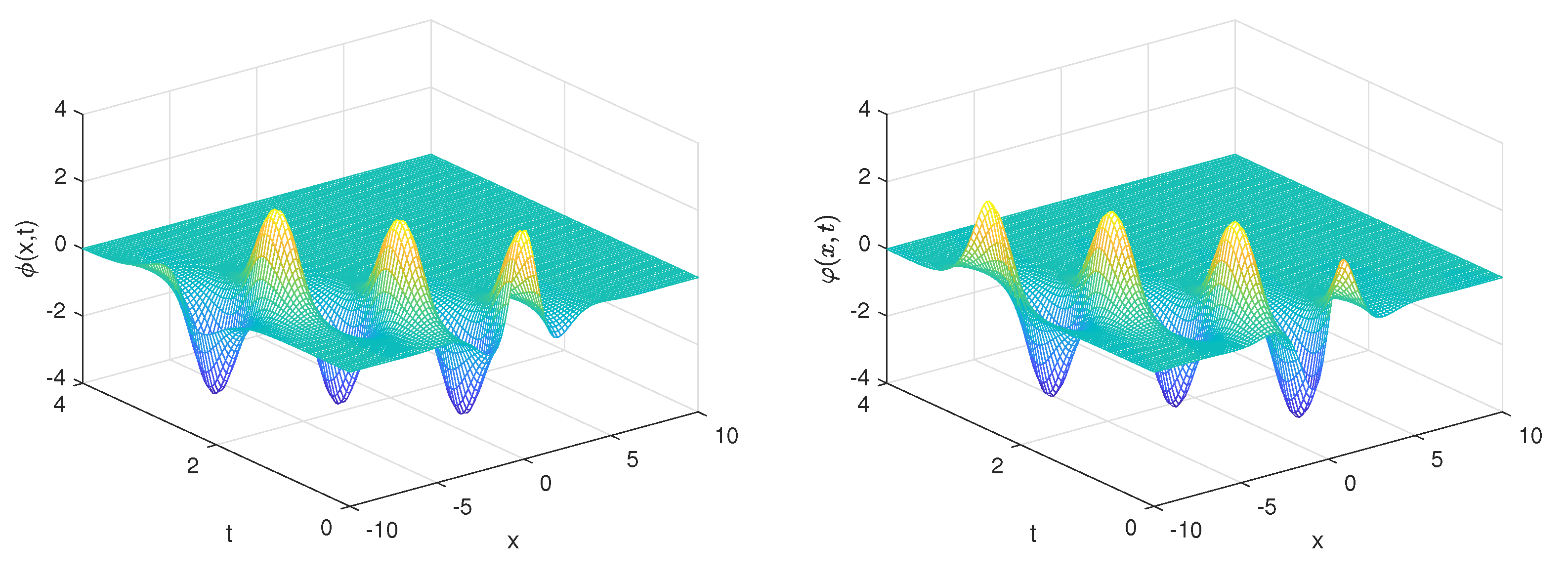
The solid curve in left panel of Figure 2 illustrates the real part of Equation (2) versus $10\le x\le -10$ at time (t) = $0.1$. The dashed curved line signifies the real function of the solution (22) for Equation (24) attained by the proposed method (LADM). One can see that the numerical solution accurately meets the obtained systematic approximation. In the right panel of Figure 2, the imaginary value of Equation (2) is compared with the numerical result obtained in Equation (23) versus $10\le x\le -10$. It shows the excitations of perturbations, keeping the carrier wave, and as a result establishes a wave packet. The surface plots of analytical solutions (22) and (23) are depicted in Figure 3. One can see that the internal fluctuations of the waves become constant and sequentially localize the solitary wave. It is important to note that the soliton excitations effect caused by a stability of steepening and the spreading impacts of the nonlinear terms. The nonlinear wave steepening influences the wave breaking for relatively insignificant wave dispersion.

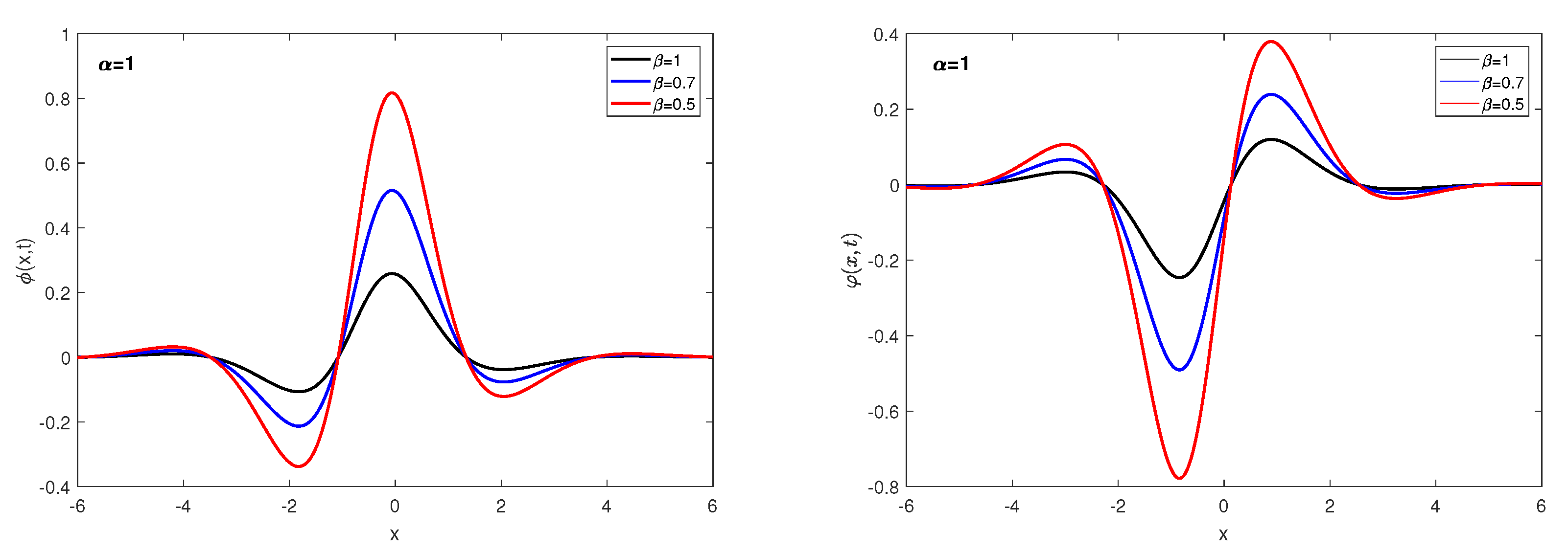
Figure 4 illustrates the influence of the fractal variable $\beta$ by fixing fractional variable $\alpha$ for time (t = 0.1) for obtained solutions $\varphi$ and $\phi$. Similarly, the influence of the variable $\alpha$ with fixed value of $\beta$ for obtained solutions $\varphi$ and $\phi$ is shown in Figure 5. In conclusion, it is found that decreasing the fractal derivative $\beta$ causes the amplitude to increase. Similarly, reducing the fractional order $\alpha$ modifies the shape of the solitonic solution and reduces its amplitude.

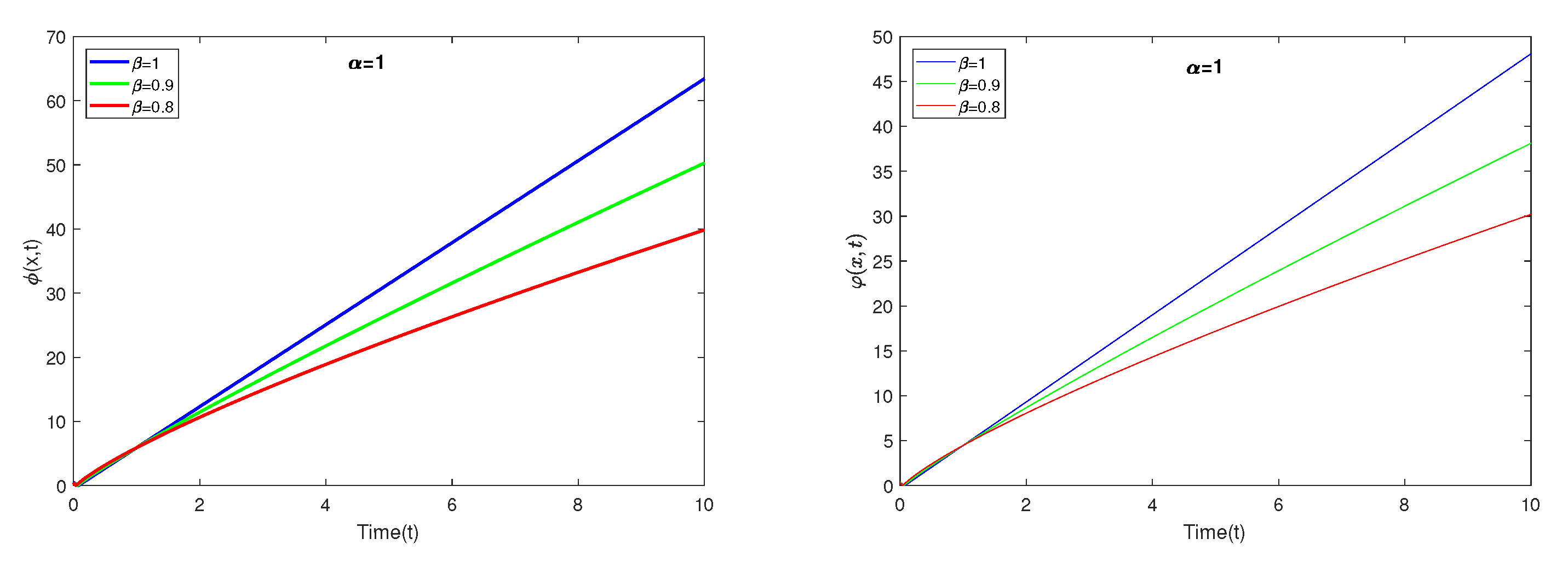
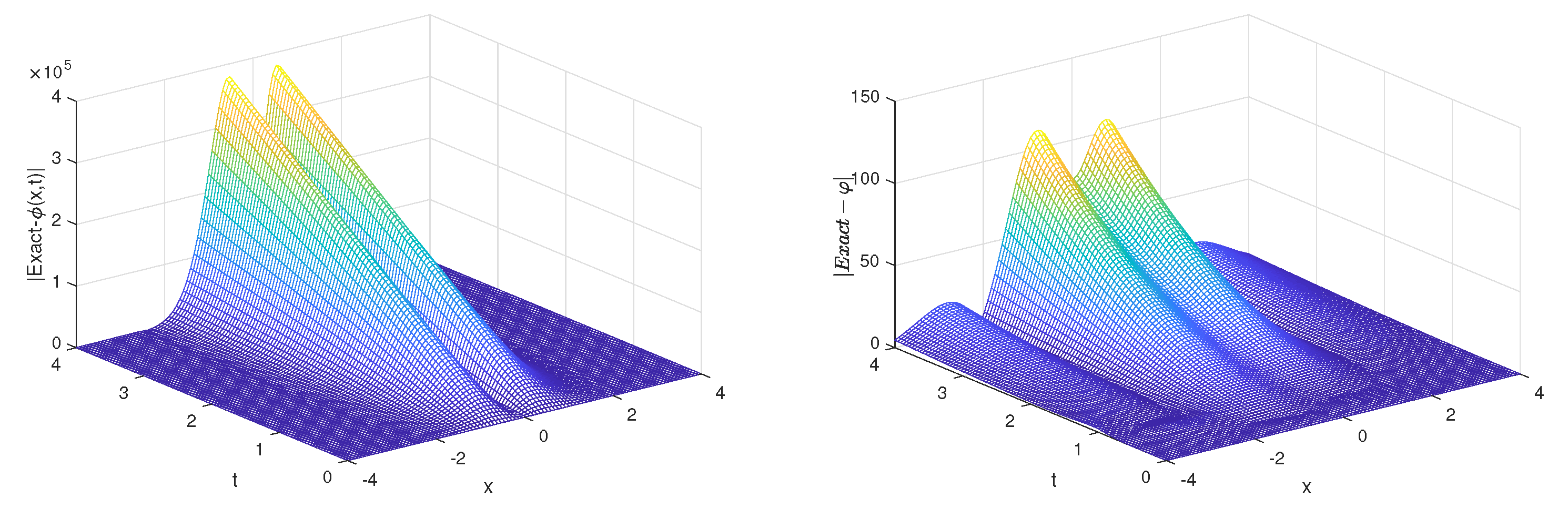
Figure 6 and Figure 7 show the behaviour of the solutions (22) and (23) with various values of $\alpha$ and $\beta$ for particular value of the spatial variables ($x=1$) versus time $\left(t\right)$. It is noted that the solitary waves are in quite good agreement for comparatively particular rate of time $\left(t\right)$. It is also found that, for $\alpha$ = $\beta$ = 1, increasing time $\left(t\right)$ rapidly increases the wave propagation. Figure 8 constitutes the surface plots of the absolute error of the solutions obtained by LADM and accurate solutions for $\varphi$ and $\phi$ for $\alpha =\beta =1$, respectively.

7. Conclusions

The coupled nonlinear system was investigated analytically and numerically with fractal fractional derivative with power law kernel. The suggested method (LADM) is applied and calculated the general series solution. The convergence analysis is also examined. For validation, a particular example is considered, and the obtained results are competed with the numerical simulation with physical interpretations. The confinement of the carrier wave and the presence of confined wave packets are observed from the numerical analysis. It is observed that the dispersion nonlinear parameter reduction equivalently influenced the wave amplitude and spatial width. It is revealed that the amplitude of the solitary wave solution increases by decreasing the fractal dimension. It is also observed that decreasing the fractional order $\alpha$ reduces the nature of the solitary wave solutions and slightly decreases the amplitude. The numerical and approximation solutions resemble effectively for specific values of time (t). However, when the fractal or fractional derivative reaches its maximum value by increasing time, the wave amplitude increases. An error analysis is performed between the obtained series solutions versus the accurate solution. It is found that the error between the exact and approximation solutions is minimized for a sufficiently small value of time $\left(t\right)$.

As a future work, it will be interesting to study the fractal fractional Hirota equation and coupled Hirota equations with variable coefficients for high-order solitary wave solution, rogue wave solution and dark–bright solutions using the Mellin transform, Chebyshev collocation scheme and Finite difference method reported in [54,55].

References

- Lu, D.; Hong, B.; Tian, L. New explicit exact solutions for the generalized coupled Hirota–Satsuma KdV system. Comput. Math. Appl. 2007, 53, 1181–1190. [Google Scholar] [CrossRef]
- Khan, K.; Ali, A.; Irfan, M.; Algahtani, O. Time-fractional electronacoustic shocks in magnetoplasma with superthermal electrons. Alex. Eng. J. 2022, 65, 531–542. [Google Scholar] [CrossRef]
- Irfan, M.; Alam, I.; Ali, A.; Shah, K.; Abdeljawad, T. Electron-acoustic solitons in dense electron-positron-ion plasma: Degenerate relativistic enthalpy function. Results Phys. 2022, 38, 105625. [Google Scholar] [CrossRef]
- Liu, G.-L. New research directions in singular perturbation theory: Artificial parameter approach and inverse-perturbation technique. In Proceedings of the 7th Conference of the Modern Mathematics and Mechanics, Shanghai, China, September 1997; Volume 61, pp. 47–53. [Google Scholar]
- He, J.H. A coupling method of homotopy technique and perturbation technique for nonlinear problems. Int. J. Non-Linear Mech. 2000, 35, 37–43. [Google Scholar] [CrossRef]
- Ali, A.; Gul, Z.; Khan, W.A.; Ahmad, S.; Zeb, S. Investigation of Fractional Order sine-Gordon Equation Using Laplace Adomian Decomposition Method. Fractals 2021, 29, 2150121. [Google Scholar] [CrossRef]
- Hirota, R. Exact envelope-soliton solutions of a nonlinear wave equation. J. Math. Phys. 1973, 14, 805–809. [Google Scholar] [CrossRef]
- Ankiewicz, A.; Soto-Crespo, J.M.; Akhmediev, N. Rogue waves and rational solutions of the Hirota equation. Phys. Rev. E 2010, 81, 046602. [Google Scholar] [CrossRef]
- Li, L.; Wu, Z.; Wang, L.; He, J. High-order rogue waves for the Hirota equation. Ann. Phys. 2013, 334, 198–211. [Google Scholar] [CrossRef]
- Anco, S.C.; Ngatat, N.T.; Willoughby, M. Interaction properties of complex modified Korteweg–de Vries (mKdV) solitons. Phys. D Nonlinear Phenom. 2011, 240, 1378–1394. [Google Scholar] [CrossRef]
- Guo, B.; Ling, L.; Liu, Q.P. Nonlinear schrödinger equation: Generalized darboux transformation and rogue wave solutions. Phys. Rev. E Stat. Nonlinear Soft Matter Phys. 2012, 85, 026607. [Google Scholar] [CrossRef]
- Zhang, Y.; Dong, K.; Jin, R. The Darboux transformation for the coupled Hirota equation. AIP Conf. Proc. 2013, 1562, 249–256. [Google Scholar]
- Huang, X. Rational solitary wave and rogue wave solutions in coupled defocusing Hirota equation. Phys. Lett. A 2016, 380, 2136–2141. [Google Scholar] [CrossRef]
- Jia, T.T.; Chai, Y.Z.; Hao, H.Q. Multi-soliton solutions and Breathers for the generalized coupled nonlinear Hirota equations via the Hirota method. Superlattices Microstruct. 2017, 105, 172–182. [Google Scholar] [CrossRef]
- Xin, W.; Yong, C. Rogue-wave pair and dark-bright-rogue wave solutions of the coupled Hirota equations. Chin. Phys. B 2014, 23, 070203. [Google Scholar]
- Chen, S. Dark and composite rogue waves in the coupled Hirota equations. Phys. Lett. A 2014, 378, 2851–2856. [Google Scholar] [CrossRef]
- Tao, Y.; He, J. Multisolitons, breathers, and rogue waves for the Hirota equation generated by the Darboux transformation. Phys. Rev. E Stat. Nonlinear Soft Matter Phys. 2012, 85, 026601. [Google Scholar] [CrossRef]
- Dai, C.; Zhang, J. New solitons for the Hirota equation and generalized higher-order nonlinear Schrödinger equation with variable coefcients. J. Phys. Math. Gen. 2013, 39, 723–737. [Google Scholar] [CrossRef]
- Bhrawy, A.H.; Alshaery, A.A.; Hilal, E.M.; Manrakhan, W.N.; Savescu, M.; Biswas, A. Dispersive optical solitons with Schrödinger-Hirota equation. J. Nonlinear Opt. Phys. Mater. 2014, 23, 1450014. [Google Scholar] [CrossRef]
- Faddeev, L.; Volkov, A.Y. Hirota equation as an example of an integrable symplectic map. Lett. Math. Phys. 1994, 32, 125–135. [Google Scholar] [CrossRef]
- Eslami, M.; Mirzazadeh, M.A.; Neirameh, A. New exact wave solutions for hirota equation. Pramana J. Phys. 2015, 84, 3–8. [Google Scholar] [CrossRef]
- Saeed, R.K.; Muhammad, R.S. Solving Coupled Hirota System by Using Homotopy Perturbation and Homotopy Analysis Methods. J. Zankoi Sulaimani-Part Pure Appl. Sci. 2015, 201, 201–2017. [Google Scholar] [CrossRef]
- Saeed, R.K.; Muhammad, R.S. Solving Coupled Hirota System by Using Variational Iteration Method. Zanco J. Pure Appl. Sci. 2015, 201, 69–80. [Google Scholar]
- Tasgal, R.S.; Potasek, M.J. Soliton solutions to coupled higher-order nonlinear Schrödinger equations. J. Math. Phys. 1992, 33, 1208–1215. [Google Scholar] [CrossRef]
- Bindu, S.G.; Mahalingam, A.; Porsezian, K. Dark soliton solutions of the coupled Hirota equation in nonlinear fiber. Phys. Lett. A 2001, 286, 321–331. [Google Scholar] [CrossRef]
- Porsezian, K.; Nakkeeran, K. Optical solitons in birefringent fibre-Backlund transformation approach. Pure Appl. Opt. 1997, 6, L7–L11. [Google Scholar] [CrossRef]
- Chen, S.H.; Song, L.Y. Rogue waves in coupled Hirota systems. Phys. Rev. E 2013, 87, 032910. [Google Scholar] [CrossRef]
- Oldham, K.B.; Spanier, J. The Fractional Calculus; Academic: New York, NY, USA, 1974. [Google Scholar]
- Podlubny, I. Fractional Differential Equations; Academic: New York, NY, USA, 1999. [Google Scholar]
- Hilfer, R. Application of Fractional Calculus in Physics; World Scientific: Singapore, 2000. [Google Scholar]
- Zaslavsky, G.M. Hamiltonian Chaos and Fractional Dynamics; Oxford University Press: Oxford, UK, 2005. [Google Scholar]
- Li, L. The cardiovascular promotion of college taekwondo based on fractional differential equation. Appl. Math. Nonlinear Sci. 2023, 8, 1577–1582. [Google Scholar] [CrossRef]
- Jiang, F. Regional Logistics Routing Optimization System Based on Fractional Differential Equation Modeling. Appl. Math. Nonlinear Sci. 2023, 8, 2865–2872. [Google Scholar] [CrossRef]
- Nishant; Bhatter, S.; Purohit, S.D.; Nisar, K.S.; Munjam, S.R. Some fractional calculus findings associated with the product of incomplete N-function and Srivastava polynomials. Int. J. Math. Comput. Eng. 2024, 2, 97–116. [Google Scholar] [CrossRef]
- Atangana, A.; Gómez-Aguilar, J.F. Numerical approximation of Riemann–Liouville definition of fractional derivative: From Riemann–Liouville to Atangana–Baleanu. Numer. Methods Partial. Differ. Equ. 2018, 34, 1502–1523. [Google Scholar] [CrossRef]
- Khader, M.M.; Saad, K.M.; Hammouch, Z.; Baleanu, D. A spectral collocation method for solving fractional KdV and KdV-Burgers equations with non-singular kernel derivatives. Appl. Numer. Math. 2021, 161, 137–146. [Google Scholar] [CrossRef]
- Atangana, A.; Baleanu, D. New fractional derivatives with nonlocal and non-singular kernel; Theory and application to heat transfer model. Therm. Sci. 2016, 20, 763–769. [Google Scholar] [CrossRef]
- Baleanu, D.; Fernandez, A.; Akgül, A. On a Fractional Operator Combining Proportional and Classical Differintegrals. Mathematics 2020, 9, 360. [Google Scholar] [CrossRef]
- Atangana, A.; Akgül, A.; Owolabi, K.M. Analysis of fractal fractional differential equations. Alex. Eng. J. 2020, 59, 1117–1134. [Google Scholar] [CrossRef]
- Atangana, A. Fractal-fractional differentiation and integration: Connecting fractal calculus and fractional calculus to predict complex system. Chaos Solit. Fractals. 2017, 102, 396–406. [Google Scholar] [CrossRef]
- Chen, W.; Sun, H.; Zhang, X.; Korošak, D. Anomalous diffusion modeling by fractal and fractional derivatives. Comput. Math. Appl. 2010, 59, 1754–1758. [Google Scholar] [CrossRef]
- Sun, H.G.; Meerschaert, M.M.; Zhang, Y.; Zhu, J.; Chen, W. A fractal Richards’ equation to capture the non-Boltzmann scaling of water transport in unsaturated media. Adv. Water Resour. 2013, 52, 292–295. [Google Scholar] [CrossRef]
- Saifullah, S.; Ali, A.; Goufo, E.F.D. Investigation of complex behaviour of fractal fractional chaotic attractor with mittag-leffler Kernel. Chaos Solitons Fract. 2021, 152, 111332. [Google Scholar] [CrossRef]
- Akgül, A.; Siddique, I. Analysis of MHD Couette flow by fractal-fractional differential operators. Chaos Solitons Fract. 2021, 146, 110893. [Google Scholar] [CrossRef]
- Atangana, A. Modelling the spread of COVID-19 with new fractal-fractional operators: Can the lockdown save mankind before vaccination? Chaos Solitons Fract. 2020, 136, 109860. [Google Scholar] [CrossRef]
- Algahtani, O.; Saifullah, S.; Ali, A. Semi-analytical and numerical study of fractal fractional nonlinear system under Caputo fractional derivative. AIMS Math. 2022, 7, 16760–16774. [Google Scholar] [CrossRef]
- Adomian, G. Solving Frontier Problems of Physics: The Decomposition Method; Kluwer Academic Publishers: Boston, MA, USA, 1995; p. 19. [Google Scholar]
- Tatari, M.; Dehghan, M. Numerical solution of Laplace equation in a disk using the Adomian decomposition method. Phys. Scr. 2005, 72, 345–348. [Google Scholar] [CrossRef]
- Andrianov, I.V.; Olevskii, V.I.; Tokarzewski, S. A modified Adomian’s decomposition method. Appl. Math. Mech. 1998, 62, 309–314. [Google Scholar] [CrossRef]
- Venkatarangan, S.N.; Rajalakshmi, K. A modification of Adomian’s solution for nonlinear oscillatory systems. Comput. Math. Appl. 1995, 29, 67–73. [Google Scholar] [CrossRef]
- Venkatarangan, S.N.; Rajalakshmi, K. Modification of Adomian’s decomposition method to solve equations containing radicals. Comput. Math. Appl. 1995, 29, 75–80. [Google Scholar] [CrossRef]
- Hussain, M.; Khan, M. Modified Laplace decomposition method. Appl. Math. Sci. 2010, 4, 1769–1783. [Google Scholar]
- Adomian, G. Modification of the decomposition approach to heat equation. J. Math. Anal. Appl. 1987, 124, 290–291. [Google Scholar] [CrossRef]
- Ata, E.; Onur Kıymaz, I. New generalized Mellin transform and applications to partial and fractional differential equations. Int. J. Math. Comput. Eng. 2023, 1, 45–66. [Google Scholar] [CrossRef]
- Demir, A.; Bayrak, M.A.; Bulut, A.; Ozbilge, E.; Çetinkaya, S. On new aspects of Chebyshev polynomials for space-time fractional diffusion process. Appl. Math. Nonlinear Sci. 2023, 8, 1051–1062. [Google Scholar] [CrossRef]
Figure 1.
(a) Comparison between exact versus approximate solutions (2)/(24) for . (b) The surface plot of approximate solution (24).
Figure 2.
(a) The real value representing accurate solution versus numerical solution from Equations (2)/(22), are depicted versus x (b) The imaginary value representing accurate solution /numerical solution from Equations (2)/(23) are depicted versus x.
Figure 3.
The wave profiles of analytical solutions (22) and (23) versus spatial and temporal variables.
Figure 4.
The influence of stable fractional order with variation in fractal variable with time for obtained solutions and .
Figure 5.
The influence of stable fractal order with variation in fractional order for the obtained solutions and at time (t).
Figure 6.
The conduct of the functions and for distinct estimates of keeping stable versus time .
Figure 7.
The behaviour of (Equation (22)) and (Equation (23)) for uneven values of by keeping stable versus time .
Figure 8.
Plot for error analysis reported in Table 1.