
Approximate Solution to Fractional Order Models Using a New Fractional Analytical Scheme


1
School of Mathematics and Statistics, Qujing Normal University, Qujing 655011, China
2
Department of Mathematics and Computer Science, University of Oradea, 1 University Street, 410087 Oradea, Romania
*
Author to whom correspondence should be addressed.
Fractal Fract. 2023, 7(7), 530; https://doi.org/10.3390/fractalfract7070530
Submission received: 4 June 2023
/
Revised: 21 June 2023
/
Accepted: 4 July 2023
/
Published: 5 July 2023
(This article belongs to the Special Issue Numerical and Exact Methods for Nonlinear Differential Equations and Applications in Physics)
Abstract
:In the present work, a new fractional analytical scheme (NFAS) is developed to obtain the approximate results of fourth-order parabolic fractional partial differential equations (FPDEs). The fractional derivatives are considered in the Caputo sense. In this scheme, we show that a Taylor series destructs the recurrence relation and minimizes the heavy computational work. This approach presents the results in the sense of convergent series. In addition, we provide the convergence theorem that shows the authenticity of this scheme. The proposed strategy is very simple and straightforward for obtaining the series solution of the fractional models. We take some differential problems of fractional orders to present the robustness and effectiveness of this developed scheme. The significance of NFAS is also shown by graphical and tabular expressions.
1. Introduction
In latest decades, partial differential problems of fractional orders have been widely used in numerous branches of sciences such as that chemical engineering, metrology, optical fibres, optimal theory, viscoelasticity, Chemotaxis and many other nonlinear models [1,2,3,4]. There have been numerous definitions of the integral and derivative of fractional orders. Various researchers have considered the Riemann, Liouville, Hadamard, and Caputo definitions as the most significant ones [5,6,7,8]. In addition to this, numerous modern definitions of the fractional derivative have been presented, but the Caputo concept continues to be the most widely used, because it has several applications in real-world phenomena [9,10]. However, the investigation of the exact solutions of these problems still pose a challenging task in various physical phenomena.
In this work, we consider the fourth-order time-fractional parabolic PDEs of the form [11,12]
where are variables subjected to the initial conditions
and boundary conditions
where and present that the functions are continuous. The parabolic equation has gone through significant improvement since it was originally used in underwater acoustics, especially regarding improvements in accuracy and its application in the domain of time. The wide-angle parabolic equation was developed to considerably reduce the phase errors of the solutions to the parabolic equation, which resemble the solution to the wave equation. The time domain parabolic problem has been extended to include wide-angle diffraction, sediment dispersion, nonlinear propagation, density variations, and sediment attenuation. The fourth-order boundary value problems have much significance in various applications of real-life problems and are being considered for the modeling of slabs of bridge, flooring patterns, wings of aviation, and frame glasses [13]. Parabolic PDEs have great importance in the analysis of viscous fluid and inflexible flows, laser distortion, and layered stretching [14].
There are numerous methods that have been studied to solve some fractional PDEs. Kheyrinataj and Nazemi [15] proposed a scheme on the basis of a neural network adaptive structure and obtained the numerical solution to the fractional differential problems. Mamehrashi [16] presented the idea of Ritz approximate strategy to derive the results of fractional control equations. Arikoglu and Ozkol [17] implemented a differential transform scheme for some composite fractional oscillation problems. Liu et al. [18] presented a multi-AUV dynamic scheme based on interval information game theory and fractional-order differential problems. Li and Zhao [19] utilized a Haar wavelet operational matrix and obtained the computational solution of some differential problems of fractional orders. The solution to these fractional problems has been obtained by numerous approaches, such as the reduced differential transform method [20], the optimal control method [21], the trial equation scheme [22], the Homotopy analysis method [23], the Melnikov method [24], the Laplace transform [25], He’s variational method [26] and the Chebyshev–Tau approach [27]. Due to some drawbacks and limitations such as restriction of the variables, assumption theory, convolution theorem, and the Lagrange multipliers in the recurrence relation, we developed an efferent approach that can overcome these drawbacks and limitations.
In the current work, we introduce a new fractional analytical scheme for the approximate solution of fourth-order parabolic FPDEs. The significant feature is that this approach computes the iteration results very quickly and close to the exact solution of the proposed problems. The obtained results are verified through 3D graphical representations and the error distribution, thus presenting the behaviour of the proposed problems under various conditions. In our model, we consider the Caputo derivative due to its common use of fractional analysis in the literature. It is used because it has a memory effect, and the derivative of a constant function becomes zero. It is also widely recognized in derivatives that fractional operators do not have the same features as a classical derivative. This work is summarized as follows: In Section 2, we reveal a few definitions of fractional calculus. We develope the idea of NFAS and present the detail for how to apply this approach to the fourth order parabolic partial differential equations in Section 3. We discuss the convergence and stability analysis of NFAS in Section 4. We illustrate three numerical applications in Section 5 to check the performance of the NAD. We summarize the results in conclusion Section 6.
2. Concepts of Fractional Calculus
In the current segment, we provide the initial concepts and ideas of fractional calculus for the development of this study [28,29].
Definition 1.
Let be a real function in space where ; then, there exists a real number such that , where , and it can be considered in space only if , where .
Definition 2.
Definition 3.
Let be a function; then, the fractional derivative in the Caputo sense is expressed as [25]
for , and .
The Caputo fractional derivative has such a significant feature such that a fractional integral is considered for an ordinary derivative to calculate the fractional order derivative, although the Riemann–Liouville fractional integral operator is linear such that
where are constants.
3. Development of New Fractional Analytical Scheme (NFAS)
In this section, we provide the development of new fractional analytical scheme for the analytical results of time-fractional fourth-order parabolic partial differential problems. Let us consider the following PDE of the fractional order
with the initial conditions
Again, implement the integration on both sides of Equation (6) to yield
This implies that
The Taylor series can be expanded for about , and we get
We can write it as
Here,
where n stands the particularly high derivative of . The endorsement of Equation (10) is to proceed the Taylor series for about . Thus,
As a result, we easily obtain the desired mathematical results.
4. Convergence and Stability Analysis of NFAS
In this section, we discuss convergence and stability analysis for the fractional problems and show that our approach is valid and authentic throughout the manuscript.
4.1. Convergence Analysis
Consider the following PDE
where Q is a nonlinear operator. The following sequence gives the identical solution such that
Theorem 1.
Let Q be an operator stating Hilbert space such that and ϑ represents the exact results of Equation (13). Then, the approximate results
yield to the exact solution ϑ when ∃ a .
Proof.
To show that is a converged Cauchy sequence, we present the following:
We start as and ; thus, we obtain
Hence, , i.e., is a Cauchy sequence in the . Thus, ∃ a s., where . □
Definition 4.
We define for every ,
4.2. Stability Analysis
Let us consider the differential problem in a Caputo fractional order sense such that
where represents the state component, and is a continuing locally Lipschitz function that satisfies . Since the initial condition is , the solution of Equation (13) starting from at time is represented by .
Additionally, since f is contiguous and locally Lipschitz, the solution of the fractional differential problem defined by Equation (13) exists. The following definitions are very important for the study of the stability of fractional differential equations.
Definition 5.
Definition 6.
The origin of the fractional differential equation defined by Equation (13) is called Mittag–Leffler stable only if the condition satisfies the following result:
where and are locally Lipschitz on a domain that satisfies .
Definition 7.
The Equation (13) is called globally continuous and asymptotically stable only if there is a function β so that for any condition, satisfies the following result:
5. Numerical Applications
This section explains the authenticity of the NFAS by illustrating some numerical applications and by stating that this scheme is reliable and accurate for obtaining the solution to fractional problems. We provide the the different behaviours of the profile solutions of the proposed models to understand the physical nature of the presented scheme. We point out that the graphical results have strong resemblance among the approximate solution and the graphical solution of the exact results.
5.1. Example 1
Consider the following equation of the FPDEs in the one-dimensional form as the following:
with initial conditions
By following the process of the NFAS, we obtain
Thus, we can obtain the following iterations
Proceeding in a similar way, we obtain
By putting the values of , we obtain
which leads to the exact solution such that
Example 1 shows the graphical representation of fourth-order parabolic PDEs in the two-dimensional form. Figure 1 is presented into two parts, where Figure 1a–c present the approximate results of for and , and Figure 1d demonstrates the precise solution of . This comparison of approximate solutions obtained by the NFAS with the exact solution has full agreement. Table 1 presents the NFAS results for distinct parameters of and reveals a high accuracy towards the precise solution.
5.2. Example 2
Consider the following equation of the FPDEs in the two-dimensional form as the following:
with initial conditions
By following the process of the NFAS, we obtain
Thus, we can obtain the following iterations
By proceeding in a similar way, we obtain
By putting the values of , we obtain
which leads to the exact solution such that
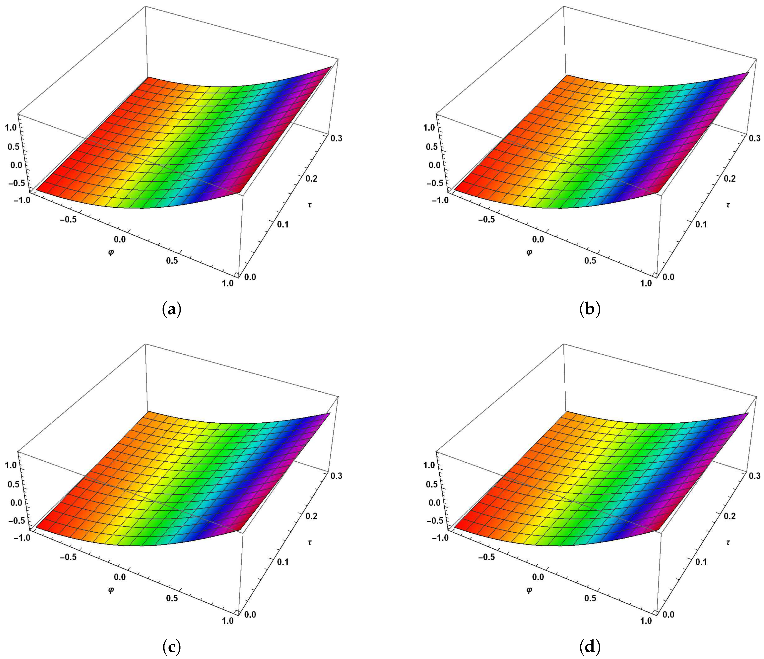
Example 2 shows the graphical representation of fourth-order parabolic PDEs in the two-dimensional form. Figure 2 is presented into two parts, where Figure 2a–c present the approximate results of for and , and Figure 2d demonstrates the precise solution of . This comparison of approximate solutions obtained by the NFAS with the exact solution has full agreement. Table 2 presents the NFAS results for distinct parameters of and reveals a high accuracy towards the precise solution.
5.3. Example 3
Consider the following equation of the FPDEs in the three-dimensional form as the following:
with initial conditions
By following the process of the NFAS, we obtain
By proceeding in a similar way, we obtain
By putting the values of , we obtain
which leads to the exact solution such that
Example 3 shows the graphical representation of fourth-order parabolic PDEs in the two-dimensional form. Figure 3 is presented into two parts, where Figure 3a–c present the approximate results of for and , and Figure 3d demonstrates the precise solution of . This comparison of approximate solutions obtained by the NFAS with the exact solution has full agreement. Table 3 presents the NFAS results for distinct parameters of and reveals a high accuracy towards the precise solution.
6. Conclusions and Future Work
In this article, we obtained the analytical results of fourth-order parabolic fractional partial differential equations with variable coefficients via a new fractional analytical scheme. The proposed algorithm is independent of any type of restriction and assumptions. We evaluated the the approximate solution of at , , and and compared it with the exact solution. We observe that the approximate solution of at has a strong agreement with the exact solution, which shows the accuracy of our proposed scheme. The rate of convergence depends on the fractional order of the differential problem. Our graphical representation and Tables show that, as the fractional order increases, the approximate solution yields to the exact solution. This scheme requires only a short number of iterations to converge to the solution. Graphical visuals and error distributions were also presented to provide the physical nature of the fourth-order fractional parabolic partial differential equations at various fractional orders. This scheme ensures the accuracy of obtaining results with the exact solutions, which has the advantage of being a direct approach to the numerical problems. In future work, we aim to use this proposed strategy for the solution of various nonlinear differential problems such as reaction–diffusion equations, the fractional KdV-Burger’s equation, the Klein–Gordon equation, and the time-fractional Boussinesq equation in terms of the Atangana–Baleanu Caputo fractional derivative operator.
Author Contributions
Investigation, Methodology, Software, and Writing—original draft, M.N.; Funding acquisition, and supervision L.F.I. All authors have read and agreed to the published version of the manuscript.
Funding
This research was funded by the University of Oradea.
Institutional Review Board Statement
Not applicable.
Informed Consent Statement
Not applicable.
Data Availability Statement
Not applicable.
Conflicts of Interest
The authors declare no conflict to interest.
References
- Wang, K.J.; Li, G.; Liu, J.H.; Wang, G.D. Solitary waves of the fractal regularized long-wave equation traveling along an unsmooth boundary. Fractals 2022, 30, 2250008. [Google Scholar] [CrossRef]
- Peng, Z.; Hu, J.; Shi, K.; Luo, R.; Huang, R.; Ghosh, B.K.; Huang, J. A novel optimal bipartite consensus control scheme for unknown multi-agent systems via model-free reinforcement learning. Appl. Math. Comput. 2020, 369, 124821. [Google Scholar] [CrossRef]
- Li, X.; Dong, Z.Q.; Wang, L.P.; Niu, X.D.; Yamaguchi, H.; Li, D.C.; Yu, P. A magnetic field coupling fractional step lattice Boltzmann model for the complex interfacial behavior in magnetic multiphase flows. Appl. Math. Model. 2023, 117, 219–250. [Google Scholar] [CrossRef]
- Jin, H.Y.; Wang, Z.A. Global stabilization of the full attraction-repulsion Keller-Segel system. Discret. Contin. Dyn.-Syst. Ser. A 2019, 40, 3509–3527. [Google Scholar] [CrossRef] [Green Version]
- Gorenflo, R.; Mainardi, F. Fractional Calculus: Integral and Differential Equations of Fractional Order; Springer: Berlin/Heidelberg, Germany, 1997. [Google Scholar]
- Kumar, S.; Kumar, A.; Samet, B.; Dutta, H. A study on fractional host–parasitoid population dynamical model to describe insect species. Numer. Methods Partial. Differ. Equ. 2021, 37, 1673–1692. [Google Scholar] [CrossRef]
- Wang, T.; Wang, G.; Yang, X.J. On a Hadamard-type fractional turbulent flow model with deviating arguments in a porous medium. Nonlinear Anal. Model. Control 2017, 22, 765–784. [Google Scholar] [CrossRef]
- Qureshi, S.; Atangana, A. Fractal-fractional differentiation for the modeling and mathematical analysis of nonlinear diarrhea transmission dynamics under the use of real data. Chaos Solitons Fractals 2020, 136, 109812. [Google Scholar] [CrossRef]
- Lyu, W.; Wang, Z.A. Global classical solutions for a class of reaction-diffusion system with density-suppressed motility. Electron. Res. Arch. 2021, 30, 995–1015. [Google Scholar] [CrossRef]
- Qureshi, S.; Kumar, P. Using Shehu integral transform to solve fractional order Caputo type initial value problems. J. Appl. Math. Comput. Mech. 2019, 18, 75–83. [Google Scholar] [CrossRef]
- AL-Jawary, M. Analytic solutions for solving fourth-order parabolic partial differential equations with variable coefficients. Int. J. Adv. Sci. Technol. Res. 2015, 3, 531–545. [Google Scholar]
- Nadeem, M.; Li, F.; Ahmad, H. Modified Laplace variational iteration method for solving fourth-order parabolic partial differential equation with variable coefficients. Comput. Math. Appl. 2019, 78, 2052–2062. [Google Scholar] [CrossRef]
- Li, J.; Chen, Y.; Liu, G. High-order compact ADI methods for parabolic equations. Comput. Math. Appl. 2006, 52, 1343–1356. [Google Scholar] [CrossRef] [Green Version]
- Nadeem, M.; Li, Z. A new strategy for the approximate solution of fourth-order parabolic partial differential equations with fractional derivative. Int. J. Numer. Methods Heat Fluid Flow 2022, 33, 1062–1075. [Google Scholar] [CrossRef]
- Kheyrinataj, F.; Nazemi, A. Fractional power series neural network for solving delay fractional optimal control problems. Connect. Sci. 2020, 32, 53–80. [Google Scholar] [CrossRef]
- Mamehrashi, K. Ritz approximate method for solving delay fractional optimal control problems. J. Comput. Appl. Math. 2023, 417, 114606. [Google Scholar] [CrossRef]
- Arikoglu, A.; Ozkol, I. Solution of fractional differential equations by using differential transform method. Chaos Solitons Fractals 2007, 34, 1473–1481. [Google Scholar] [CrossRef]
- Liu, L.; Wang, J.; Zhang, L.; Zhang, S. Multi-AUV dynamic maneuver countermeasure algorithm based on interval information game and fractional-order DE. Fractal Fract. 2022, 6, 235. [Google Scholar] [CrossRef]
- Li, Y.; Zhao, W. Haar wavelet operational matrix of fractional order integration and its applications in solving the fractional order differential equations. Appl. Math. Comput. 2010, 216, 2276–2285. [Google Scholar] [CrossRef]
- Wang, K.L.; Wang, K.J. A modification of the reduced differential transform method for fractional calculus. Therm. Sci. 2018, 22, 1871–1875. [Google Scholar] [CrossRef] [Green Version]
- Luo, R.; Peng, Z.; Hu, J. On model identification based optimal control and it’s applications to multi-agent learning and control. Mathematics 2023, 11, 906. [Google Scholar] [CrossRef]
- Pandir, Y.; Ekin, A. New solitary wave solutions of the Korteweg-de Vries (KdV) equation by new version of the trial equation method. Electron. J. Appl. Math. 2023, 1, 101–113. [Google Scholar]
- Zurigat, M.; Momani, S.; Odibat, Z.; Alawneh, A. The homotopy analysis method for handling systems of fractional differential equations. Appl. Math. Model. 2010, 34, 24–35. [Google Scholar] [CrossRef]
- Zhang, J.; Xie, J.; Shi, W.; Huo, Y.; Ren, Z.; He, D. Resonance and bifurcation of fractional quintic Mathieu–Duffing system. Chaos Interdiscip. J. Nonlinear Sci. 2023, 33, 23131. [Google Scholar] [CrossRef] [PubMed]
- Kexue, L.; Jigen, P. Laplace transform and fractional differential equations. Appl. Math. Lett. 2011, 24, 2019–2023. [Google Scholar] [CrossRef] [Green Version]
- Wang, K.J.; Wang, G.D. He’s variational method for the time–space fractional nonlinear Drinfeld–Sokolov–Wilson system. Math. Methods Appl. Sci. 2023, 46, 7798–7806. [Google Scholar] [CrossRef]
- Nejla, G.; Emine, G.K.; Yusuf, G. Chebyshev-Tau method for the linear Klein-Gordon equation. Int. J. Phys. Sci. 2012, 7, 5723–5728. [Google Scholar]
- Sarikaya, M.Z.; Ogunmez, H. On new inequalities via Riemann-Liouville fractional integration. Abstr. Appl. Anal. 2012, 2012, 428983. [Google Scholar] [CrossRef]
- Farid, G. Some Riemann–Liouville fractional integral inequalities for convex functions. J. Anal. 2019, 27, 1095–1102. [Google Scholar] [CrossRef]
- Liu, Q.; Peng, H.; Wang, Z.A. Convergence to nonlinear diffusion waves for a hyperbolic-parabolic chemotaxis system modelling vasculogenesis. J. Differ. Equ. 2022, 314, 251–286. [Google Scholar] [CrossRef]
- Ali, K.K.; Maneea, M. New approximation solution for time-fractional Kudryashov-Sinelshchikov equation using novel technique. Alex. Eng. J. 2023, 72, 559–572. [Google Scholar] [CrossRef]
- Sene, N. Exponential form for Lyapunov function and stability analysis of the fractional differential equations. J. Math. Comput. Sci. 2018, 18, 388–397. [Google Scholar] [CrossRef] [Green Version]
- Khan, A.; Syam, M.I.; Zada, A.; Khan, H. Stability analysis of nonlinear fractional differential equations with Caputo and Riemann-Liouville derivatives. Eur. Phys. J. Plus 2018, 133, 264. [Google Scholar] [CrossRef]
- Hattaf, K. On the stability and numerical scheme of fractional differential equations with application to biology. Computation 2022, 10, 97. [Google Scholar] [CrossRef]
Figure 1.
Graphical relation of the approximate solution with the precise solution for distinct parameters of . (a) Graphical visual of approximate solution for . (b) Graphical visual of approximate solution for . (c) Graphical visual of approximate solution for . (d) Graphical visual of precise solution.
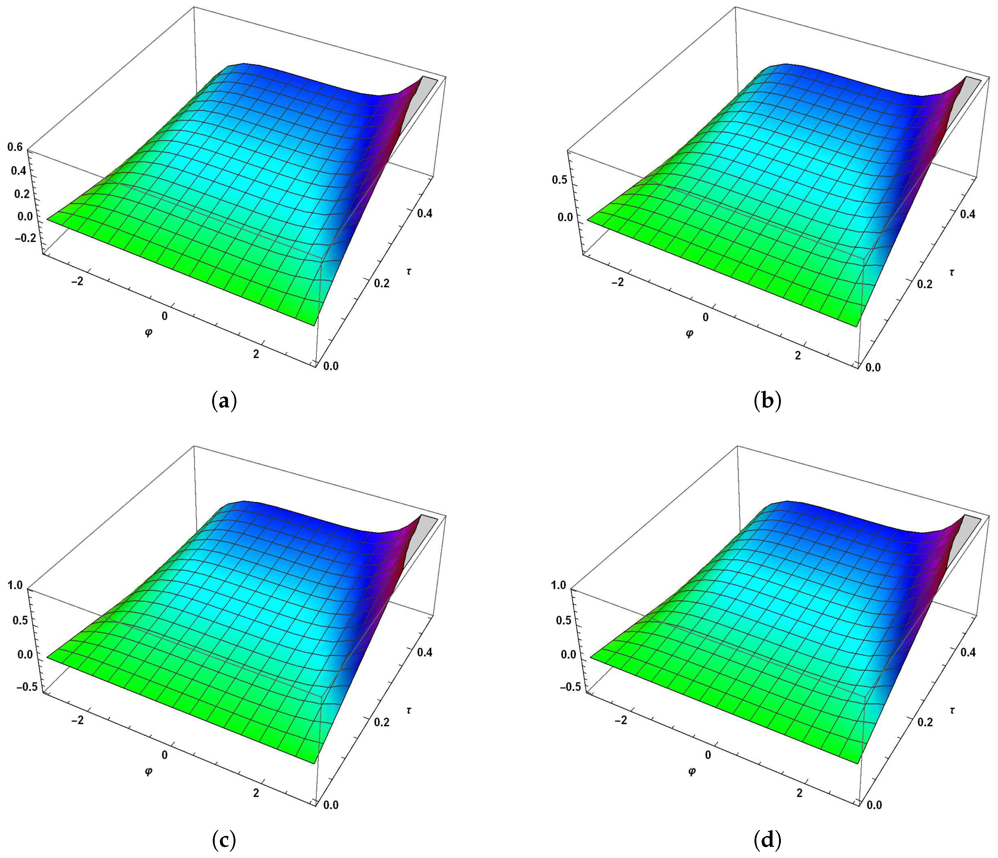
Figure 2.
Graphical relation of the approximate solution with the precise solution for distinct parameters of . (a) Graphical visual of approximate solution for . (b) Graphical visual of approximate solution for . (c) Graphical visual of approximate solution for . (d) Graphical visual of precise solution.

Figure 3.
Graphical relation of the approximate solution with the precise solution for distinct parameters of . (a) Graphical visual of approximate solution for . (b) Graphical visual of approximate solution for . (c) Graphical visual of approximate solution for . (d) Graphical visual of precise solution.


Table 1.
The NFAS results for distinct parameters of when for Example 1.
| Exact Solution | ||||
|---|---|---|---|---|
| 0.10 | 0.190039 | 0.274522 | 0.29552 | 0.29552 |
| 0.15 | 0.190039 | 0.274522 | 0.29552 | 0.29552 |
| 0.20 | 0.190039 | 0.274523 | 0.29551 | 0.29551 |
| 0.25 | 0.190040 | 0.274524 | 0.295523 | 0.295523 |
| 0.30 | 0.190042 | 0.274528 | 0.295526 | 0.295526 |
| 0.35 | 0.190047 | 0.274534 | 0.295533 | 0.295533 |
| 0.40 | 0.190055 | 0.274545 | 0.295545 | 0.295545 |
| 0.45 | 0.0190068 | 0.274564 | 0.295566 | 0.295566 |
| 0.50 | 0.190088 | 0.274594 | 0.295597 | 0.295597 |
Table 2.
The NFAS results for distinct parameters of when and for Example 2.
| Exact Solution | ||||
|---|---|---|---|---|
| 0.10 | 0.380073 | 0.549038 | 0.591034 | 0.591034 |
| 0.15 | 0.380073 | 0.549038 | 0.591034 | 0.591034 |
| 0.20 | 0.380073 | 0.549038 | 0.591034 | 0.591034 |
| 0.25 | 0.380073 | 0.549038 | 0.591034 | 0.591034 |
| 0.30 | 0.380073 | 0.549038 | 0.591034 | 0.591034 |
| 0.35 | 0.380073 | 0.549039 | 0.591035 | 0.591035 |
| 0.40 | 0.380074 | 0.549040 | 0.591036 | 0.591036 |
| 0.45 | 0.380075 | 0.549041 | 0.591037 | 0.591037 |
| 0.50 | 0.380077 | 0.549044 | 0.591040 | 0.591040 |
Table 3.
The NFAS results for distinct parameters of when , , and for Example 3.
| Exact Solution | ||||
|---|---|---|---|---|
| 0.10 | −1.56817 | −1.47581 | −1.42272 | −1.42272 |
| 0.15 | −1.51193 | −1.41958 | −1.36648 | −1.36648 |
| 0.20 | −1.45323 | −1.36087 | −1.30778 | −1.30778 |
| 0.25 | −1.39208 | −1.29972 | −1.24662 | −1.24662 |
| 0.30 | −1.3285 | −1.23614 | −1.18305 | −1.18305 |
| 0.35 | −1.26254 | −1.17018 | −1.11708 | −1.11708 |
| 0.40 | −1.19422 | −1.10187 | −1.04877 | −1.04877 |
| 0.45 | −1.12361 | −1.03125 | −0.978158 | −0.978158 |
| 0.50 | −1.05075 | −0.958389 | −0.905293 | −0.905293 |
Disclaimer/Publisher’s Note: The statements, opinions and data contained in all publications are solely those of the individual author(s) and contributor(s) and not of MDPI and/or the editor(s). MDPI and/or the editor(s) disclaim responsibility for any injury to people or property resulting from any ideas, methods, instructions or products referred to in the content. |
© 2023 by the authors. Licensee MDPI, Basel, Switzerland. This article is an open access article distributed under the terms and conditions of the Creative Commons Attribution (CC BY) license (https://creativecommons.org/licenses/by/4.0/).
Share and Cite
MDPI and ACS Style
Nadeem, M.; Iambor, L.F. Approximate Solution to Fractional Order Models Using a New Fractional Analytical Scheme. Fractal Fract. 2023, 7, 530. https://doi.org/10.3390/fractalfract7070530
AMA Style
Nadeem M, Iambor LF. Approximate Solution to Fractional Order Models Using a New Fractional Analytical Scheme. Fractal and Fractional. 2023; 7(7):530. https://doi.org/10.3390/fractalfract7070530
Chicago/Turabian StyleNadeem, Muhammad, and Loredana Florentina Iambor. 2023. "Approximate Solution to Fractional Order Models Using a New Fractional Analytical Scheme" Fractal and Fractional 7, no. 7: 530. https://doi.org/10.3390/fractalfract7070530