


Bifurcation of Traveling Wave Solution of Sakovich Equation with Beta Fractional Derivative

Department of Mathematics and Statistics, College of Science, King Faisal University, P.O. Box 400, Al-Ahsa 31982, Saudi Arabia
*
Author to whom correspondence should be addressed.
Fractal Fract. 2023, 7(5), 372; https://doi.org/10.3390/fractalfract7050372
Submission received: 10 March 2023
/
Revised: 23 April 2023
/
Accepted: 27 April 2023
/
Published: 29 April 2023
(This article belongs to the Special Issue Recent Advances in Time/Space-Fractional Evolution Equations)
Abstract
:The current work is devoted to studying the dynamical behavior of the Sakovich equation with beta derivatives. We announce the conditions of problem parameters leading to the existence of periodic, solitary, and kink solutions by applying the qualitative theory of planar dynamical systems. Based on these conditions, we construct some new solutions by integrating the conserved quantity along the possible interval of real wave propagation in order to obtain real solutions that are significant and desirable in real-world applications. We illustrate the dependence of the solutions on the initial conditions by examining the phase plane orbit. We graphically show the fractional order beta effects on the width of the solutions and keep their amplitude approximately unchanged. The graphical representations of some 3D and 2D solutions are introduced.
1. Introduction
In recent years, time evolution phenomena, such as nonlinear waves, are best described by partial differential equations [1,2]. These equations are hard to analyze, and there are no common analytical approaches to solve them. Exact traveling wave solutions of nonlinear evolution equations are one of the fundamental objects of study in mathematical physics. These exact solutions, when they exist, can help one to understand the mechanism of the complicated physical phenomena and dynamical processes modeled by these nonlinear evolution equations. Among traveling wave solutions, solitary waves with nonlinear dispersive effects, called solitons, are of great interest due to their additional property of permanently retaining [3,4]. Solitons play a momentous role in the telecommunication industry as signals can proceed far away without any distortion in the form of solitons, see for example [5]. As a sequence, numerous techniques have been proposed in the literature to obtain different solutions [6,7,8,9,10,11,12,13]. The Korteweg–de Vries (KdV) equation and its modifications are nonlinear differential equations, whose solutions were analytically described. The family of the KdV equations model a number of nonlinear processes such as waves in shallow water, ion acoustic waves in plasma, and many physics and engineering phenomena [14,15]. In his work on the Painlevé analysis of a class of second-order equations, Sakovich formed a new equation using the KdV-equation and the fifth order KdV-equation [16]. The equation obtained, named after Sakovich, takes the following form:
where u is a wave function in three independent variables, representing time and two spatial variables. The Sakovich equation was extended several time to obtain versions with more independent variables [17,18]. It is worth noting that the Sakovich equation and all its extended versions are Painlevé integrable [16,17,18]. The Painlevé test [19] provides a criterion for the integrability of nonlinear partial differential equations. In [16], Sakovich showed that Equation (1) satisfies the Painlevé test and possesses multiple solutions that satisfy, simultaneously, the Korteweg–de Vries (KdV) equation and the fifth-order KdV equation.
In fact, numerous evolutionary systems with memory effects on dynamics have been mathematically modeled using fractional calculus. Several different derivative definitions such as Riemman–Liouville, Caputo, Grünwald–Letnikov, etc., have arisen (see for example [20,21]. Fractional derivatives have their geometric and physical interpretations [22]. In [23], Atangana introduced the “beta-derivative”, which complies with numerous requirements that were restrictions for fractional derivatives. The introduced derivative can be thought of as a natural extension of the classical derivative rather than fractional derivatives. For more information about the -derivative, see Appendix A. The -derivative version of Equation (1) is given by
where and represents the -derivative with respect to space and time, respectively. Notice, when , Equation (2) will be reduced to Equation (1). The solutions for several fractional nonlinear equations were investigated in the literature [24,25]. Bifurcation is one of the methods used to describe the solutions of many fractional and classical differential equations [26,27,28,29,30,31,32,33,34,35]. In this work, we use bifurcation methods to investigate the dynamical behavior of Equation (2). To the extent of the authors’ knowledge, the study of the -time derivative Sakovich equation has not been investigated in the literature. We construct some wave solutions of the equation, and study the influence of the order -derivative on the obtained solutions.
This paper is organized as follows: Section 2 contains the mathematical analysis covering the conversion of Equation (2) into a traveling wave system by using appropriate wave transformation and applying the qualitative theory for a planar integrable system to this system. Section 3 is devoted to constructing a wave solution for Equation (2). In Section 4, we provide 3D-graphical representations and illustrate the effect of the order on the solutions. Finally, Section 5 gives a summary of the obtained result.
2. Bifurcation Analysis
We search for a wave solution in the form
where are arbitrary constants and is the Gamma function. Applying Proposition A2, we obtain
where primes indicate a derivative with respect to . Taking into account the results provided in the appendix, and the expressions (4), we obtain
Thus, we have two possibilities, either , or . The first equation, , gives a solution of the form
where are two constants. The second equation
can be written as a dynamical system in the form
Since H does not explicitly depend on , which plays the role of the time in Hamiltonian mechanics, it is a conserved quantity, i.e., it takes a constant value along all the phase orbits. Thus, we obtain
where f is an arbitrary constant. Using Equation (12), we can rewrite the first equation in (9) as
where is given by
To integrate both sides of Equation (13), we need to determine the range of the parameters , and f. The desired range can be determined by using bifurcation analysis. For more details about the bifurcation theory, see, e.g., [36,37]. First, we find the equilibrium points for the Hamiltonian system (9). These are the critical points for the potential function (11), i.e., they are , where satisfies the quadratic equation . The number of the equilibrium points is determined by the sign of the discriminant . We will consider the different possibilities individually and utilize MATLAB software to sketch phase portraits:
- (a)
- If , then there is a unique equilibrium point for system (9). This point is a cusp since . The phase portrait and potential function for system (9) are shown in Figure 1a,b, respectively. For fixed values of the parameters , there are three type of phase orbits depending on whether , shown in blue, , shown in green, or , shown in red, where is the value of the conserved quantity at the cusp point . All the phase orbits in these cases are unbounded and, consequently, they will imply unbounded solutions.
- (b)
- If , then there are no equilibrium points for the Hamiltonian system (9). The phase plane consists of one family of unbounded phase orbits for any value of the parameter f as shown in Figure 2a. This type of phase orbit will lead to unbounded solutions. The potential function (11) is given by Figure 2b.
- (c)
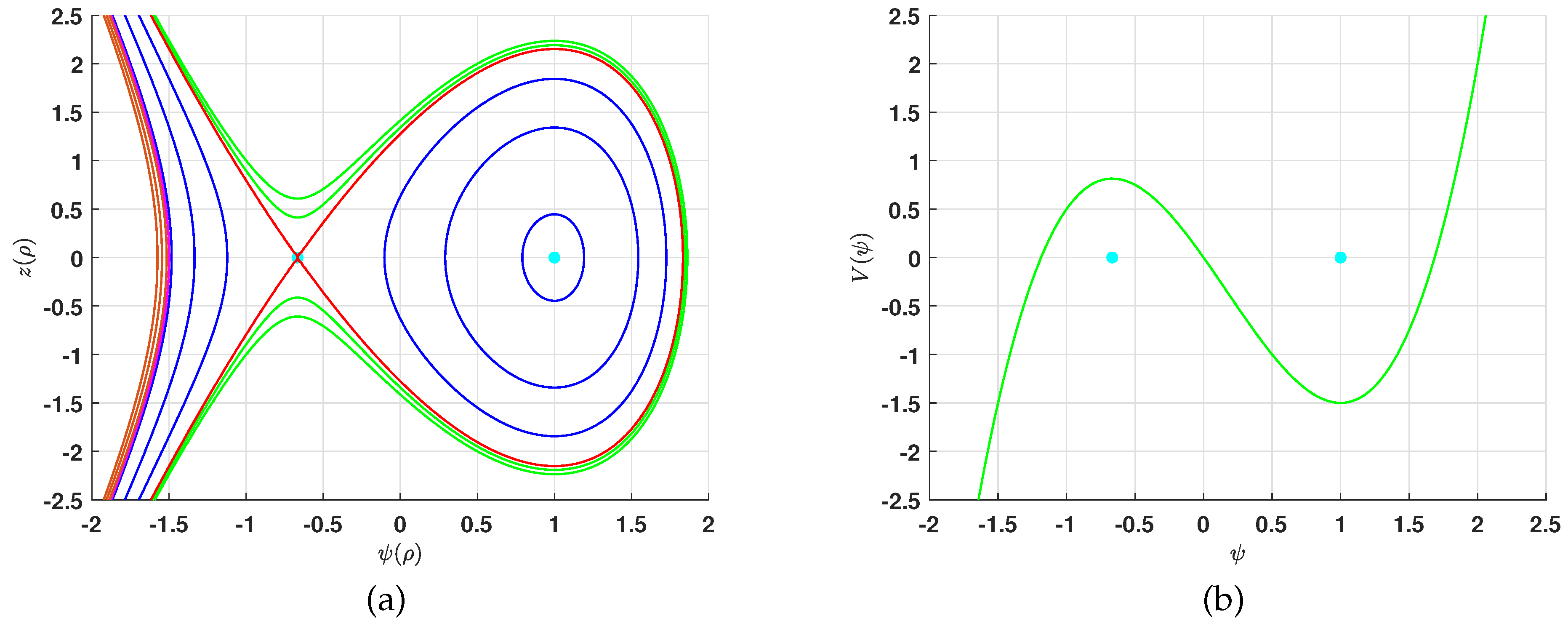
- If , then there are two equilibrium points for the Hamiltonian system (9). They are . To determine the nature of these equilibrium points, we calculateSince reversing the signs of k and exchanges and , we may assume , hence . Under this assumption, will be a center while will be a saddle point. Figure 3a,b show the phase portrait and potential function (11), respectively. To describe the phase portrait for this case, we defined the two constants and , which are the values of the conserved quantity at the equilibrium points , i.e.,
Figure 1.
(a) Phase portrait when () and (b) the potential function. The cyan solid circle is the equilibrium point.
Figure 1.
(a) Phase portrait when () and (b) the potential function. The cyan solid circle is the equilibrium point.
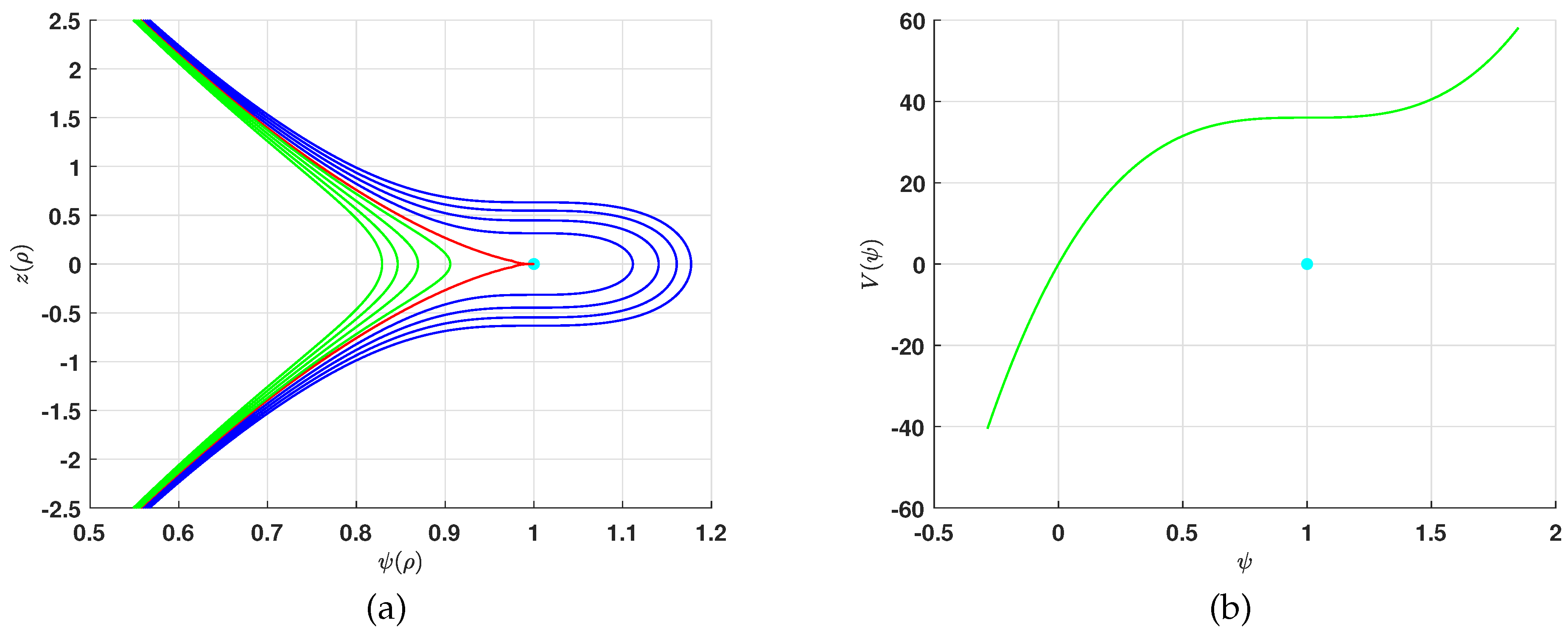
Figure 2.
(a) Phase portrait when () and (b) the potential function.

Figure 3.
(a) Phase portrait when with () and (b) the potential function. The cyan solid circles are the equilibrium points.
Figure 3.
(a) Phase portrait when with () and (b) the potential function. The cyan solid circles are the equilibrium points.
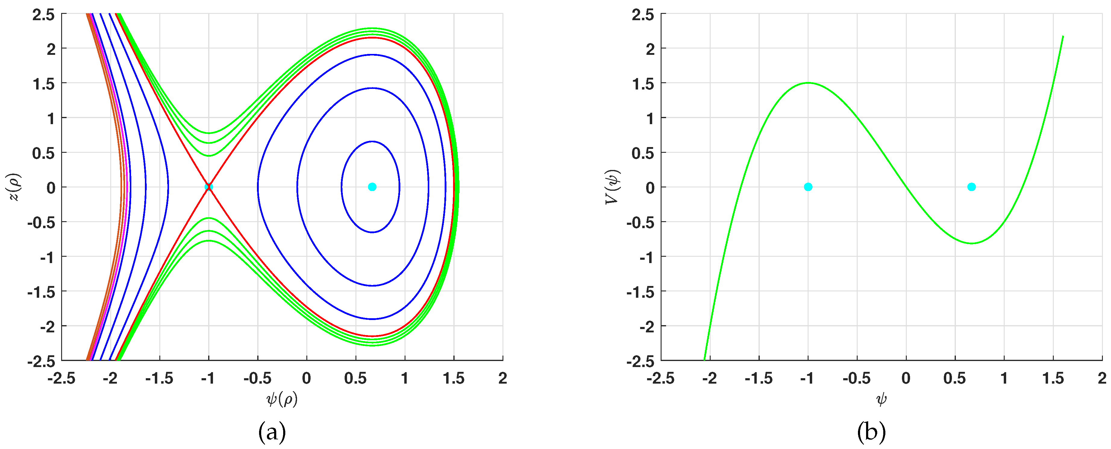
For all the energy levels , system (9) has a family of unbounded orbits, shown in green in Figure 3a. Corresponding to the energy level , there is a homoclinic orbit, shown in red, which connects the saddle point with itself and has unbounded extensions. For , there are two families of orbits, shown in blue, one of which is periodic enclosing the center point and contained inside the homoclinic orbit while the other one is unbounded. For , there is a single unbounded orbit, shown in pink. Finally, when , there is a family of unbounded orbits, shown in brown.
3. Solutions
The present section aims to obtain solutions for Equation (2) taking into account the bifurcations constraints on the parameters introduced in the previous section. Equation (13) can be written as
where
The procedure of finding the solutions is given in the following Theorems:
Theorem 1.
Proof.
- (a)
- For the given range of the parameters, system (9) has two families of unbounded orbits shown in blue and in green in Figure 1a. This shows that the polynomial (18) has one real root and two complex conjugate roots , where denotes the complex conjugate. Note that if while if . The domain of the solution in both cases is . Assuming , and integrating both sides of Equation (17), we obtain the solution of Equation (2) given in (19).
- (b)
- For the selected range of the parameters, system (9) has a single phase orbit passing through the cusp point , shown in red in Figure 1a. This shows that the polynomial (18) has as a repeated root. Hence, . The domain of the solution is . Assuming , and integrating both sides of Equation (2) gives us the solution (20).
□
Proof.
For the given range of the parameters, system (9) has no equilibrium point as shown in Figure 2a and any phase orbit intersects the –axis at exactly one point. Thus, the polynomial (18) has one real root , and two complex conjugate roots . The domain of the solution is . Assuming and integrating both sides of Equation (17), we obtain a solution in the form (19) for Equation (2). □
Theorem 3.
Assuming , we have
Proof.
- (a)
- For the given range of the parameters, system (9) has a homoclinic orbit, shown in red in Figure 3a. This shows that the polynomial (18) has one double root, which is , and another simple root denoted by . Thus, . There are two possible domains of the solution . If and , then integrating both sides of Equation (17) gives the solution (21). If and , we obtain the solution (22) by integrating both sides of Equation (17).
- (b)
- The bifurcation analysis shows that for the given range of the parameters, the system (9) has two families of orbits; one is periodic and the other unbounded. This shows that the polynomial (18) has three real zeros, , where . Thus, . There are two possible domains of the solution, namely . Assuming , , and integrating both sides of Equation (17), we obtain a new solution (23) for Equation (2). On other hand, if , , then integrating both sides of Equation (13) yields to a new solution (24) for Equation (2).
- (c)
- The proof of this statement is completely analogous to the proof of part (a) in Theorem 1.
□
The next proposition gives the procedures of obtaining the solutions for Equation (2) corresponding to the phase orbits shown in Figure 4a.
Proposition 1.
Remark 1.
Note that the roots after carrying out the replacement in Proposition 1 are different from those in Theorem 3 due to the dependence of the roots on the coefficients of the polynomial (18). Thus, the solutions obtained in Proposition 1 are different from those in Theorem 3.
Finding the domain of the solution is important since it enables us to construct all possible solutions for Equation (2). This deserves some elaboration. It should be noted that from part (a) in Theorem 3, we have two solutions, (21) and (22), for the same conditions on the parameters , and f, that are completely different mathematically and physically. Solution (22) is a solitary solution that corresponds to the red homoclinic phase orbit in Figure 3a. The other solution (21) is unbounded and corresponds to the unbounded extension of the homoclinic orbit. The two solutions are the results of integrating Equation (17) along all possible intervals of real wave propagation.
Remark 2.
The degeneracy of the obtained solutions can be investigated through the transition between the phase plane orbits. This shows the consistency of the obtained results. In Figure 3a, when , the periodic family of blue orbits will be transformed to the homoclinic orbit, shown in red. Thus, the periodic solution (24) corresponding to a periodic orbit will be transformed to the solitary solution (22). The correctness of this statement can be seen by letting , then and , and the solution (24) converges to:
which agrees with the solution (22).
4. Graphical Representation
In this sections, we give 2D and 3D representations of the solutions obtained above and clarify the influence of the fractional order on the solutions.
For the fixed values and , m is restricted to fall in the interval . We will take . The solution of Equation (2) can be obtained from Theorem 3 as determined by the value of the conserved quantity (12) and the domain of the solution. We have the following cases:
- (a)
- For , Equation (2) has either the solution (21) or (22) depending on the chosen domain of the solution. Thus, if we select , where are the zeros of the polynomial (18), then Equation (2) has the solution (22), which can be rewritten in the formSolution (26) is a solitary wave solution for Equation (2) corresponding to the homoclinic orbit in red as outlined by Figure 3a. This type of solutions is also named a compressive solitary wave solution; for more details, see, e.g., [36]. Figure 5a–c show the 3D-graphical representation of the solution (26) for several values of the order () while Figure 5d shows the 2D representation of the solutions. It should be noted that the amplitude of the solution is left approximately unchanged by changing the value of the order while the solution’s width decreases with the increasing of the order .
- (b)
- We take , which falls in the interval . From Theorem (3), Equation (2) has either the solution (23) or the solution (24) depending on the chosen domain of the solution. Direct calculations give , , and , which are the roots of the polynomial (18). Choosing the interval of the real solution as , will result in the solution for Equation (2) having the formThe solution (27) is a periodic solution for Equation (2) and this solution corresponds to the periodic family of orbit in blue around the equilibrium point as is clarified by Figure 3a. Figure 6a–c show the 3D-graphical representation of the solution (27) for different values of () while Figure 6d shows the 2D representation of the solution. Figure 6d shows that the amplitude of the solution (27) remains unchanged for changing values of the order while the solution’s width decreases as the value of the order increases.
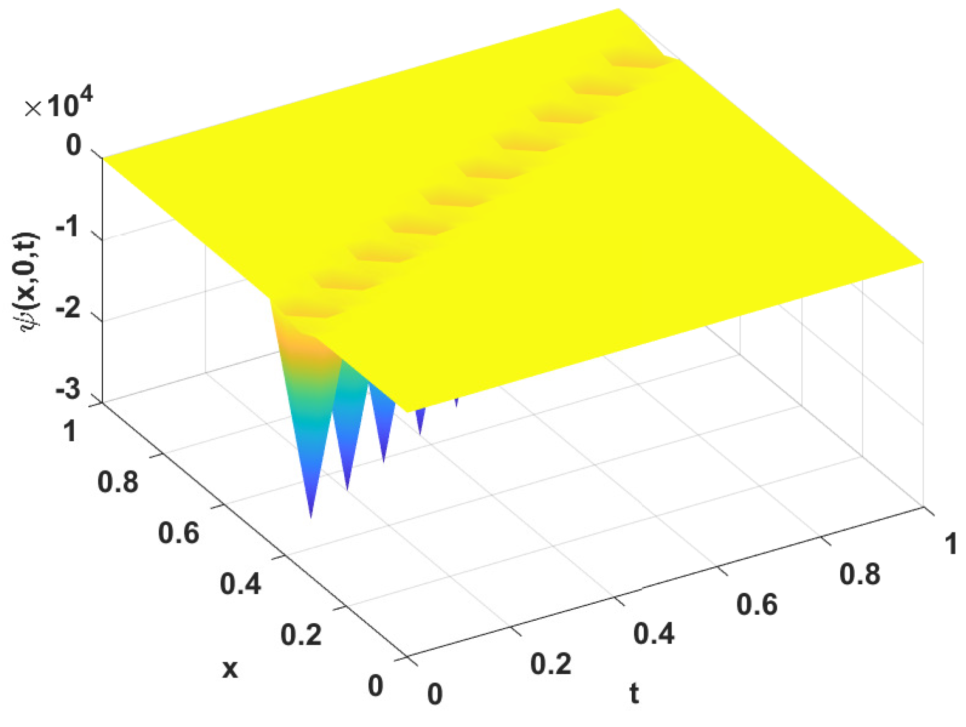
To illustrate the importance of the choice of the domain of the solution, we give the graphical representation for two solutions having the same condition on the parameters, but with different domains of the solution. The solution (23) with takes the form
The two solutions (27) and (28) were obtained with the same conditions on the parameters , and , but with different domains of the solution. The two solutions are completely different physically and mathematically, as shown in Figure 6a and Figure 7. One of them is periodic and the other is singular. This can be also seen by examining the phase orbits. The phase orbit for this case consists of two orbits, shown in blue in Figure 3a. One of the orbits is periodic, which gives a periodic solution, and the other is unbounded, which gives an unbounded solution.
Figure 5.
Graphic representation of the solution (22) for different values of the fractional order . (a) . (b) . (c) . (d) 2D representation with various .
Figure 5.
Graphic representation of the solution (22) for different values of the fractional order . (a) . (b) . (c) . (d) 2D representation with various .

Figure 6.
Graphic representation of the solution (24) for different values of the fractional order . (a) . (b) . (c) . (d) 2D representation with various .
Figure 6.
Graphic representation of the solution (24) for different values of the fractional order . (a) . (b) . (c) . (d) 2D representation with various .
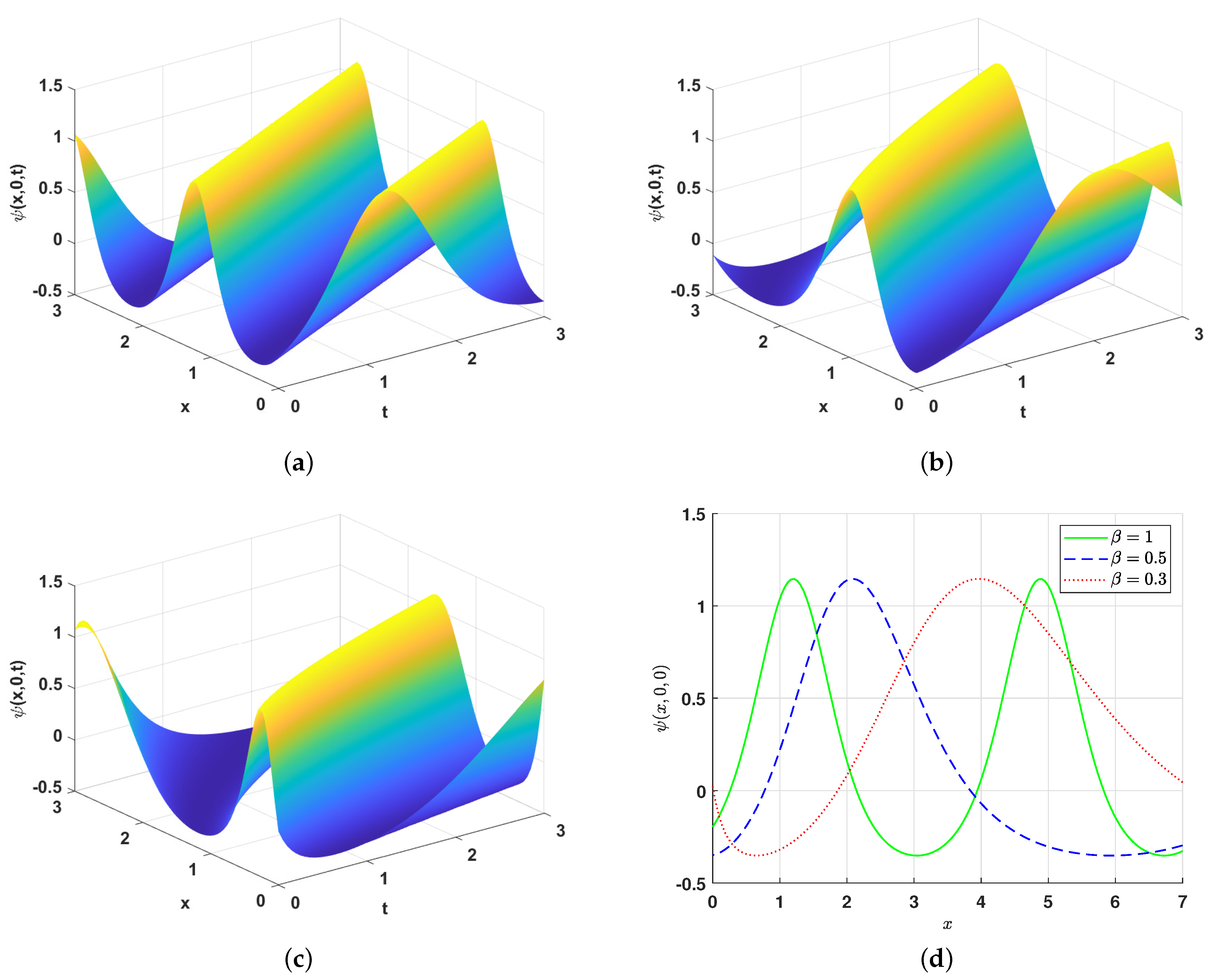
Figure 7.
Graphic representation of the solution (23) with .
Figure 7.
Graphic representation of the solution (23) with .
5. Conclusions
This paper studied the dynamical behavior of the solutions of the fractional Sakovich equation with beta derivatives for time and space variables. This equation was transformed in an appropriate manner to create a Hamiltonian system that describes time evolution. Bifurcation analysis was carried out, the phase portrait was generated, and possible domains of the solution were determined. To create some novel solutions for the Sakovich equation with beta derivatives, the conserved quantity was integrated along these intervals. The dependence of the solutions on the initial conditions was illustrated by examining the phase plane orbit. The 3D- and 2D-graphical representations of these solutions were generated. We showed that the fractional order affected the width of the solitary and periodic solutions while leaving the amplitude of the solutions approximately unchanged. Furthermore, we have illustrated the significance of the choice of the domain of the solution by producing two solutions with the same conditions on the parameters, but with different domains of the solution. We have found that one of them is periodic while the other is singular, i.e., they are mathematically and physically different, as shown in Figure 6a and Figure 7. This point also illustrated the effectiveness of applying bifurcation analysis since the latter solutions correspond to the phase orbit in blue, in Figure 3a, which consists of two families, where one of them is periodic and the other is unbounded. The upcoming work may include the study of chaotic behavior for system (9) after adding the periodic term and its applications to image encryption. Additionally, the geometric and physical interpretation for Equation (2) will be considered.
Author Contributions
Conceptualization, M.A.N.; Methodology, M.A.N. and M.A.A.; Software, M.A.A. and M.A.N.; Validation, M.A.N. and M.A.A.; Formal analysis, M.A.N. and M.A.A.; Writing—original draft, M.A.N. and M.A.A.; Writing—review & editing, M.A.A. and M.A.N.; Funding acquisition, M.A.A. All authors have read and agreed to the published version of the manuscript.
Funding
The authors extend their appreciation to the Deputyship for Research and Innovation, Ministry of Education in Saudi Arabia for funding this research work through the project number INST193.
Data Availability Statement
The data that support the findings of this study are available from the author upon reasonable request.
Acknowledgments
The authors acknowledge the Deputyship for Research & Innovation, Ministry of Education in Saudi Arabia for their financial support, project number INST193.
Conflicts of Interest
The author declare that they have no competing interest.
Appendix A. β-Derivative
The importance of fraction calculus stems from it great applicability in modeling natural phenomena. Different fractional integrals and derivatives have been defined [24,38]. Among these definitions, the -derivative was defined as follows:
Definition A1
If the above limit exists for a function f and , we say that f is -differentiable. We list some properties of the -fractional derivatives in the following proposition. To simplify notations, we omitted the index 0 and use for .
Proposition A1
- 1.
- for all scalars .
- 2.
- .
- 3.
- For , we have .
- 4.
- For any constant c, .
The following lemma can be directly proved using the definition of -derivative and the substitution
Lemma A1.
Let , and f be a differentiable and β-differentiable function, then
Theorem A1.
Let be a differentiable and —differentiable function. Assume g is a function defined in the range of f and also differentiable. Then, we have
Proof.
Let , then
□
Note that fractional derivatives can be considered a natural extension of the classical derivatives ().
In the following, we extend -derivative to include functions of several variables as follows:
Note that if , we obtain . The proofs of the results in the following can be done using the definition above and the substitution .
Proposition A2.
Let , and be two β-differentiable functions. The following statements hold.
- 1.
- 2.
- .
- 3.
- For , we have.
References
- Christiansen, P.; Sørensen, M.P.; Scott, A.C. Nonlinear Science at the Dawn of the 21st Century; Lecture Notes in Physics; Springer: Berlin/Heidelberg, Germany, 2000; Volume 542. [Google Scholar]
- Al Nuwairan, M.; Chaabelasri, E. Balanced Meshless Method for Numerical Simulation of Pollutant Transport by ShallowWater Flow over Irregular Bed: Application in the Strait of Gibraltar. Appl. Sci. 2022, 12, 6849. [Google Scholar] [CrossRef]
- Kilic, B.; Inc, M. Optical solitons for the Schrödinger–Hirota equation with power law nonlinearity by the Bäcklund transformation. Optik 2017, 138, 64–67. [Google Scholar] [CrossRef]
- İnç, M.; Kilic, B.; Baleanu, D. Optical soliton solutions of the pulse propagation generalized equation in parabolic-law media with space-modulated coefficients. Optik 2016, 127, 1056–1058. [Google Scholar] [CrossRef]
- Inc, M. New compacton and solitary pattern solutions of the nonlinear modified dispersive Klein–Gordon equations. CHaos Solitons Fractals 2007, 33, 1275–1284. [Google Scholar] [CrossRef]
- Hirota, R. Exact solution of the Kortewegde Vries equation for multiple collisions of solitons. Phys. Rev. Lett. 1971, 27, 1192. [Google Scholar] [CrossRef]
- Liu, S.; Fu, Z.; Liu, S.; Zhao, Q. Jacobi elliptic function expansion method and periodic wave solutions of nonlinear wave equations. Phys. Lett. A 2001, 289, 69–74. [Google Scholar] [CrossRef]
- Ma, W.X.; Batwa, S. A binary Darboux transformation for multicomponent NLS equations and their reductions. Anal. Math. Phys. 2021, 11, 44. [Google Scholar] [CrossRef]
- Kumar, S.; Dhiman, S.K.; Baleanu, D.; Osman, M.S.; Wazwaz, A.M. Lie symmetries, closed-form solutions, and various dynamical profiles of solitons for the variable coefficient (2+1)-dimensional KP equations. Symmetry 2022, 14, 597. [Google Scholar] [CrossRef]
- Fan, E.; Zhang, J. Applications of the Jacobi elliptic function method to special-type nonlinear equations. Phys. Lett. 2002, 305, 383–392. [Google Scholar] [CrossRef]
- Rabie, W.; Ahmed, H.; Hamdy, W. Exploration of New Optical Solitons in Magneto-Optical Waveguide with Coupled System of Nonlinear Biswas–Milovic Equation via Kudryashov’s Law Using Extended F-Expansion Method. Mathematics 2023, 11, 300. [Google Scholar] [CrossRef]
- Asghar, A.; Seadawy, A. Dispersive soliton solutions for shallow water wave system and modified Benjamin-Bona-Mahony equations via applications of mathematical methods. J. Ocean Eng. Sci. 2021, 6, 85–98. [Google Scholar]
- Aderyani, S.; Saadati, R.; O’Regan, D.; Alshammari, F. Describing Water Wave Propagation Using the G′/G2—Expansion Method. Mathematics 2023, 11, 191. [Google Scholar] [CrossRef]
- Darrigol, O. Worlds of Flow: A history of hydrodynamics from the Bernoullis to Prandtl; Oxford University Press: New York, NY, USA, 2009. [Google Scholar]
- Seadawy, A.R.; Iqbal, M.; Lu, D. Propagation of kink and anti-kink wave solitons for the nonlinear damped modified Korteweg–de Vries equation arising in ion-acoustic wave in an unmagnetized collisional dusty plasma. Phys. Stat. Mech. Its Appl. 2020, 544, 123560. [Google Scholar] [CrossRef]
- Sakovich, S. A New Painlevé-Integrable Equation Possessing KdV-Type Solitons. Nonlinear Phenom. Complex Syst. 2019, 22, 299–304. Available online: https://arxiv.org/abs/1907.01324 (accessed on 1 March 2023).
- Wang, G.; Wazwaz, A.M. Symmetry and Painlevé analysis for the extended Sakovich equation. Int. J. Numer. Methods Heat Fluid Flow 2020, 31, 541–547. [Google Scholar] [CrossRef]
- Wazwaz, A.M. Two new Painlevé integrable extended Sakovich equations with (2+1) and (3+1) dimensions. Int. J. Numer. Methods Heat Fluid Flow 2019, 30, 1379–1387. [Google Scholar] [CrossRef]
- Weiss, J.; Tabor, M.; Carnevale, G. The Painlevé property for partial differential equations. J. Math. Phys. 1983, 24, 522–526. [Google Scholar] [CrossRef]
- Caputo, M.; Fabricio, M. A new definition of fractional derivative without singular kernel. Prog. Fract. Differ. Appl. 2015, 1, 73–85. [Google Scholar]
- Atangana, A.; Secer, A. A note on fractional order derivatives and table of fractional derivatives of some special functions. Abstr. Appl. Anal. 2013, 2013, 279681. [Google Scholar] [CrossRef]
- Podlubny, I. Geometric and physical interpretation of fractional integration and fractional differentiation. Fract. Calc. Appl. Anal. 2002, 5, 367–386. [Google Scholar]
- Atangana, A.; Baleanu, D.; Alsaedi, A. Analysis of time-fractional hunter-saxton equation: A model of neumatic liquid crystal. Open Phys. 2016, 14, 145–149. [Google Scholar] [CrossRef]
- Das, S. Functional Fractional Calculus; Springer: Berlin/Heidelberg, Germany, 2011; Volume 1. [Google Scholar]
- Tarasov, V.E. Fractional Dynamics: Applications of Fractional Calculus to Dynamics of Particles, Fields and Media; Springer Science (Business Media): New York, NY, USA, 2011. [Google Scholar]
- Elmandouh, A.A.; Elbrolosy, M.E. New traveling wave solutions for Gilson–Pickering equation in plasma via bifurcation analysis and direct method. Math. Methods Appl. Sci. 2022, 2022, 1–15. [Google Scholar] [CrossRef]
- Al Nuwairan, M.; Elmandouh, A. Qualitative analysis and wave propagation of the nonlinear model for low-pass electrical transmission lines. Phys. Scr. 2021, 96, 095214. [Google Scholar] [CrossRef]
- Elmandouh, A.; Elbrolosy, M. Integrability, variational principal, bifurcation and new wave solutions for Ivancevic option pricing model. J. Math. 2022, 2022, 9354856. [Google Scholar] [CrossRef]
- Al Nuwairan, M. Bifurcation and Analytical Solutions of the Space-Fractional Stochastic Schrödinger Equation with White Noise. Fractal Fract. 2023, 7, 157. [Google Scholar] [CrossRef]
- Elbrolosy, M.E.; Elmandouh, A. Dynamical behaviour of conformable time-fractional coupled Konno-Oono equation in magnetic field. Math. Probl. Eng. 2022, 2022, 3157217. [Google Scholar] [CrossRef]
- Hassan, T.S.; Elmandouh, A.A.; Attiya, A.A.; Khedr, A.Y. Bifurcation Analysis and Exact Wave Solutions for the Double-Chain Model of DNA. J. Math. 2022, 2022, 7188118. [Google Scholar] [CrossRef]
- Alhamud, M.; Elbrolosy, M.; Elmandouh, A. New Analytical Solutions for Time-Fractional Stochastic (3+1)-Dimensional Equations for Fluids with Gas Bubbles and Hydrodynamics. Fractal Fract. 2023, 7, 16. [Google Scholar] [CrossRef]
- Aldhafeeri, A.; Al Nuwairan, M. Bifurcation of Some Novel Wave Solutions for Modified Nonlinear Schrödinger Equation with Time M-Fractional Derivative. Mathematics 2023, 11, 1219. [Google Scholar] [CrossRef]
- Du, L.; Sun, Y.; Wu, D. Bifurcations and solutions for the generalized nonlinear Schrödinger equation. Phys. Lett. A 2019, 383, 126028. [Google Scholar] [CrossRef]
- Han, T.; Li, Z.; Zhang, X. Bifurcation and new exact traveling wave solutions to time-space coupled fractional nonlinear Schrödinger equation. Phys. Lett. A 2021, 395, 127217. [Google Scholar] [CrossRef]
- Saha, A.; Banerjee, S. Dynamical Systems and Nonlinear Waves in Plasmas; CRC Press: Boca Raton, FL, USA, 2021; p. x+207. [Google Scholar]
- Nemytskii, V.V. Qualitative Theory of Differential Equations; Princeton University Press: Princeton, NJ, USA, 2015; Volume 2083. [Google Scholar]
- Miller, K.S.; Ross, B. An Introduction to the Fractional Calculus and Fractional Differential Equations; Wiley-Blackwell: Hoboken, NJ, USA, 1993. [Google Scholar]
- Artin, E. The Gamma Function; Library of Congress (English Translation): Washington, DC, USA, 1964.
- Atangana, A.; Alqahtani, R. Modelling the Spread of River Blindness Disease via the Caputo Fractional Derivative and the Beta-derivative. Entropy 2016, 18, 40. [Google Scholar] [CrossRef]
Figure 4.
(a) Phase portrait when with () and (b) the potential function. The cyan solid circles are the equilibrium points.
Figure 4.
(a) Phase portrait when with () and (b) the potential function. The cyan solid circles are the equilibrium points.
Disclaimer/Publisher’s Note: The statements, opinions and data contained in all publications are solely those of the individual author(s) and contributor(s) and not of MDPI and/or the editor(s). MDPI and/or the editor(s) disclaim responsibility for any injury to people or property resulting from any ideas, methods, instructions or products referred to in the content. |
© 2023 by the authors. Licensee MDPI, Basel, Switzerland. This article is an open access article distributed under the terms and conditions of the Creative Commons Attribution (CC BY) license (https://creativecommons.org/licenses/by/4.0/).
Share and Cite
MDPI and ACS Style
Almulhim, M.A.; Al Nuwairan, M. Bifurcation of Traveling Wave Solution of Sakovich Equation with Beta Fractional Derivative. Fractal Fract. 2023, 7, 372. https://doi.org/10.3390/fractalfract7050372
AMA Style
Almulhim MA, Al Nuwairan M. Bifurcation of Traveling Wave Solution of Sakovich Equation with Beta Fractional Derivative. Fractal and Fractional. 2023; 7(5):372. https://doi.org/10.3390/fractalfract7050372
Chicago/Turabian StyleAlmulhim, Munirah A., and Muneerah Al Nuwairan. 2023. "Bifurcation of Traveling Wave Solution of Sakovich Equation with Beta Fractional Derivative" Fractal and Fractional 7, no. 5: 372. https://doi.org/10.3390/fractalfract7050372