Characterization of the Local Growth of Two Cantor-Type Functions

Abstract

The Cantor set and its homonymous function have been frequently utilized as examples for various physical phenomena occurring on discontinuous sets. This article characterizes the local growth of the Cantor’s singular function by means of its fractional velocity. It is demonstrated that the Cantor function has finite one-sided velocities, which are non-zero of the set of change of the function. In addition, a related singular function based on the Smith–Volterra–Cantor set is constructed. Its growth is characterized by one-sided derivatives. It is demonstrated that the continuity set of its derivative has a positive Lebesgue measure of 1/2.

1. Introduction

The Cantor set is an example of a perfect set (i.e., closed and having no isolated points) that is at the same time nowhere dense. The Cantor set and its homonymous function have been frequently utilized as examples for various physical phenomena occurring on discontinuous sets. The self-similar properties of the Cantor set allow for convenient simplifications when developing such models. For example, the Cantor function arises in models of mechanical stability and damage of quasi-brittle materials [1], in the mechanics of disordered elastic materials [2,3] or in fluid flows in fractally permeable reservoirs [4].

The homonymous function was introduced by Georg Cantor in 1883, as a counterexample to then-prevalent opinion about the universal applicability of the Fundamental Theorem of Calculus. The Cantor function is the standard example of a singular function whose derivative vanishes almost everywhere in the unit interval. In particular, the Cantor’s function is an example of a function that is continuous, but not absolutely continuous. Therefore, characterization of the Cantor’s function in terms of local fractional calculus or the closely related fractional velocity has its own merits. On the other hand, the construction of the Cantor set can be generalized in a way that gives rise to a singular function, called here the SVC (Smith–Volterra–Cantor) function for brevity, with somehow more physically realistic properties. Notably, its growth can be characterized by the usual notion of derivative suitably relaxed to allow for discontinuities.

There are different naming conventions for the Cantor function in the literature. The same function is also called sometimes the Cantor ternary function, the Lebesgue function, Lebesgue’s singular function, the Cantor–Vitali function, the Devil’s staircase, the Cantor staircase function and the Cantor–Lebesgue function. Expositions about properties of the function can be found in [5,6].

On $I=[0,1]$, Cantor’s function can be defined as the solution of the functional equation

$$F\left(x\right):=\frac{1}{2}\left\{\begin{array}{cc}F\left(3x\right),\hfill & 0\le x\le 1/3\hfill \\ 1\hfill & 1/3<x<2/3\hfill \\ F(3x-2)+1,\hfill & 2/3\le x\le 1\hfill \end{array}\right.$$

(1)

The function is the unique solution of Equation (1) in the class of all bounded functions $f:[0;1]\mapsto \mathbb{R}$ ([7,8] (Proposition 10.6.2)). It has fixed points $F\left(0\right)=0$ and $F\left(1\right)=1$, among others. The symbol F without subscripts is reserved for the Cantor function throughout the manuscript. The function is skew-symmetric about the point $1/2$ according to the equation [9]:

$$F\left(x\right)+F(1-x)=1$$

(2)

Outside the unit interval the function can be analytically continued. Typically, one can adjoin the interval $U=[-\infty ,0]$ to the domain of F by assigning $F\left(y\right)=0,y\in U$ and $V=[0,\infty ]$ to the domain of F by assigning $F\left(y\right)=\lfloor y\rfloor +F\left(\left\{y\right\}\right),y\in V$, where $\lfloor y\rfloor$ and $\left\{y\right\}$ represent the integral and the fractional part of the number y, respectively.

From a different perspective, the Cantor function can be defined also as the map between the Cantor ternary set $\mathcal{C}$ and the set of dyadic rationals $\mathcal{D}\setminus \{1/2\}$ extended by continuity on the entire unit interval. This approach will be used for the second example presented in the paper.

2. Bounds of Growth of the Cantor’S Function

The Cantor function grows on the Cantor set. The Cantor set is a classical example of a perfect subset of the closed interval [0, 1] that has the same cardinality as the real line but whose Lebesgue measure is zero.

Definition 1.

We say that f is of (point-wise) Hölder class ${\mathbb{H}}^{\beta }$ if for a given x there exist two positive constants $C,\delta \in \mathbb{R}$ that for an arbitrary y in its domain and given $|x-y|\le \delta$ fulfil the inequality $|f\left(x\right)-f\left(y\right)|\le {C|x-y|}^{\beta }$, where $|·|$ denotes the norm of the argument.

Cantor’s function is Hölder continuous on every point of the Cantor set. Moreover, the point-wise Hölder exponent $\alpha =log2/log3\approx 0.63092975$. Everywhere in the paper $\alpha$ will be treated as a constant with this value. Moreover, this exponent coincides with the Hausdorff dimension of the Cantor set.

Here we establish a useful bound for the Cantor’s function oscillation on I.

• Upper bond of$F\left(x\right).$ By the functional Equation (1) and the monotonicity $F\left(x\right)\le x^{\alpha }$.
• Lower bond$F\left(x\right).$ For $x=\frac{2}{3^n}$ we have $F\left(\frac{2}{3^n}\right)=\frac{1}{2^n}$. Therefore, since F is increasing,

  $$F\left(x\right)\ge {\left(\frac{x}{2}\right)}^{\alpha }.$$

The relationship between $L\left(x\right):={\left(\frac{x}{2}\right)}^{\alpha }$, $F\left(x\right)$ and $U\left(x\right):=x^{\alpha }$ is plotted in Figure 1a. Therefore,

$${\left(\frac{x}{2}\right)}^{\alpha }\le F\left(x\right)\le x^{\alpha }$$

(3)

By composing Equations (2) and (3) we arrive at another bonding estimate for $F\left(x\right)$:

$$1-U(1-x)\le F\left(x\right)\le 1-L(1-x)$$

(4)

The relationship is plotted in Figure 1b. Finally, $\forall x\in I$

$$1-U(1-x)\le F\left(x\right)\le U\left(x\right)$$

(5)

3. Point-Wise Oscillation of Functions

Unless otherwise stated, everywhere in the paper $ϵ$ will be considered a positive real number.

Definition 2

(Anonymous function notation). The notation for the pair $\mu ::ϵ$ will be interpreted as the implication that if the left-hand side, is fixed then the right-hand side, is fixed by the value chosen on the left, i.e., as an anonymous functional dependency $ϵ=ϵ\left(\mu \right)$.

Definition 3.

Define the forward oscillation and its limit as the operators

$$\begin{array}{cc}\hfill {\mathrm{osc}}_{ϵ}^{+}\left[f\right]\left(x\right):=& \underset{[x,x+ϵ]}{sup}f-\underset{[x,x+ϵ]}{inf}f,I=[x,x+ϵ]\hfill \\ \hfill {\mathrm{osc}}^{+}\left[f\right]\left(x\right):=& \underset{ϵ\to 0}{lim}\left(\underset{I}{sup}-\underset{I}{inf}\right)f=\underset{ϵ\to 0}{lim}\left(\underset{I}{sup}f-\underset{I}{inf}f\right)\hfill \end{array}$$

and the backward oscillation and its limit as the operators

$$\begin{array}{cc}\hfill {\mathrm{osc}}_{ϵ}^{-}\left[f\right]\left(x\right):=& \underset{[x-ϵ,x]}{sup}f-\underset{[x-ϵ,x]}{inf}f,I=[x-ϵ,x]\hfill \\ \hfill {\mathrm{osc}}^{-}\left[f\right]\left(x\right):=& \underset{ϵ\to 0}{lim}\left(\underset{I}{sup}-\underset{I}{inf}\right)f=\underset{ϵ\to 0}{lim}\left(\underset{I}{sup}f-\underset{I}{inf}f\right)\hfill \end{array}$$

according to previously introduced notation [10,11].

Lemma 1

(Oscillation lemma). Consider the function $f:X\mapsto Y\subseteq {\mathbb{R}}^{}$. Suppose that $I_{+}=\left[x,x+ϵ\right]\subseteq X$, $I_{-}=\left[x-ϵ,x\right]\subseteq X$, respectively.

If ${\mathrm{osc}}^{+}\left[f\right]\left(x\right)=0$ then f is right-continuous at x. Conversely, if f is right-continuous at x then ${\mathrm{osc}}^{+}\left[f\right]\left(x\right)=0$. If ${\mathrm{osc}}^{-}\left[f\right]\left(x\right)=0$ then f is left-continuous at x. Conversely, if f is left-continuous at x then ${\mathrm{osc}}^{-}\left[f\right]\left(x\right)=0$. That is,

$$\underset{ϵ\to 0}{lim}{\mathrm{osc}}_{ϵ}^{\pm }\left[f\right]\left(x\right)=0⟺\underset{ϵ\to 0}{lim}f(x\pm ϵ)=f\left(x\right)$$

Proof. 

Forward case Suppose that ${\mathrm{osc}}_{}^{+}\left[f\right]\left(x\right)=0$. Then there exists a pair $\mu ::\delta ,\delta \le ϵ$, such that ${\mathrm{osc}}_{\delta }^{+}\left[f\right]\left(x\right)\le \mu$. Therefore, f is bounded in $I_{+}$. Since $\mu$ is arbitrary, we select $x^{\prime }$ such that

$$|f\left(x^{\prime }\right)-f\left(x\right)|={\mu }^{\prime }\le \mu$$

and set $|x-x^{\prime }|={\delta }^{\prime }$. Since $\mu$ can be made arbitrarily small, so is ${\mu }^{\prime }$. Therefore, f is (right)-continuous at x.

Reverse case. If f is (right-) continuous at $x\in I=[x,x+ϵ]$ then there exists a pair $\mu ::\delta$ such that

$$\begin{array}{cc}\hfill \left|f\left(x^{\prime }\right)-f\left(x\right)\right|& <\mu /2,\left|x^{\prime }-x\right|<\delta /2\hfill \\ \hfill \left|f\left(x\right)-f\left(x^{\prime \prime }\right)\right|& <\mu /2,\left|x-x^{\prime \prime }\right|<\delta /2\hfill \end{array}$$

for some $x^{\prime },x^{\prime \prime }\in I$, which are different from x. Then we add the inequalities and by the triangle inequality we have

$$\begin{array}{cc}\hfill \left|f\left(x^{\prime }\right)-f\left(x^{\prime \prime }\right)\right|& \le \left|f\left(x^{\prime }\right)-f\left(x\right)\right|+\left|f\left(x\right)-f\left(x^{\prime \prime }\right)\right|<\mu \hfill \\ \hfill \left|x^{\prime }-x^{\prime \prime }\right|& \le \left|x^{\prime }-x\right|+\left|x-x^{\prime \prime }\right|<\delta .\hfill \end{array}$$

However, since $x^{\prime }$ and $x^{″}$ are arbitrary we can set the former to correspond to the minimum and the latter to the maximum of f in the interval. Therefore, by the least-upper-bond property we can identify $f\left(x^{\prime }\right)\mapsto {inf}_{ϵ}f\left(x\right)$, $f\left(x^{\prime \prime }\right)\mapsto {sup}_{ϵ}f\left(x\right)$. Therefore, ${\mathrm{osc}}_{\delta }^{+}\left[f\right]\left(x\right)<\mu$ for $\left|x^{\prime }-x^{″}\right|<\delta$ (for the pair $\mu ::\delta$ ). Therefore, the limit is ${\mathrm{osc}}^{+}\left[f\right]\left(x\right)=0$.

The left case follows by applying the right case, just proved, to the mirrored image of the function: $f(-x)$.  □

Then the negation of the statement is also true:

Corollary 1.

The following statements are equivalent

$${\mathrm{osc}}_{}^{\pm }\left[f\right]\left(x\right)=\underset{ϵ\to 0}{lim}{\mathrm{osc}}_{ϵ}^{\pm }\left[f\right]\left(x\right)>0⟺\underset{ϵ\to 0}{lim}f(x\pm ϵ)\ne f\left(x\right)$$

Definition 4.

Define the set of discontinuity for the function f in the compact interval I of Lebesgue measure |I| as

$$\Delta [f,I]:=\left\{x:{\mathrm{osc}}_{}^{\pm }\left[f\right]\left(x\right)>0,x\in I\right\}$$

or if the context is known $\Delta [f,I]\equiv \Delta \left[I\right]$. In particular, under this definition ${\mathrm{osc}}_{}^{\pm }\left[f\right]\left(x\right)=\infty$ is admissible.

From this definition it is apparent that $|\Delta [F\left]\right|=0$ and $|\Delta [F^{\prime }\left]\right|=0$ on $I=[0,1]$.

4. Fractional Velocity

In the late 20th century, Cherbit introduced fractional velocity as a tool to study the fractal phenomena and physical processes for which instantaneous velocity was not well defined [12]. The properties of fractional velocity have been extensively studied in [10,13]. It was established that for fractional orders fractional velocity is continuous only if it is zero. The properties of fractional velocity are surveyed in [11].

Definition 5.

Define the parametrized difference operators acting on a function $f\left(x\right)$ as

$$\begin{array}{cc}\hfill {\Delta }_{ϵ}^{+}\left[f\right]\left(x\right)& :=f(x+ϵ)-f\left(x\right),\hfill \\ \hfill {\Delta }_{ϵ}^{-}\left[f\right]\left(x\right)& :=f\left(x\right)-f(x-ϵ)\hfill \end{array}$$

where $ϵ>0$. The first one we refer to as forward difference operator, the second one we refer to as backward difference operator.

Definition 6.

Define Fractal Variation operators of order $0<\beta \le 1$ as

$$\begin{array}{c}\hfill {\upsilon }_{ϵ+}^{\beta }\left[f\right]\left(x\right):=\frac{{\Delta }_{ϵ}^{+}\left[f\right]\left(x\right)}{{ϵ}^{\beta }}=\frac{f(x+ϵ)-f\left(x\right)}{{ϵ}^{\beta }}\end{array}$$

(6)

$$\begin{array}{c}\hfill {\upsilon }_{ϵ-}^{\beta }\left[f\right]\left(x\right):=\frac{{\Delta }_{ϵ}^{-}\left[f\right]\left(x\right)}{{ϵ}^{\beta }}=\frac{f\left(x\right)-f(x-ϵ)}{{ϵ}^{\beta }}\end{array}$$

(7)

for a positive ϵ [14].

Definition 7

(Fractional order velocity). Define the fractional velocity of fractional order β as the limit

$$\begin{array}{cc}\hfill {\upsilon }_{\pm }^{\beta }f\left(x\right)& :=\underset{ϵ\to 0}{lim}\frac{{\Delta }_{ϵ}^{\pm }\left[f\right]\left(x\right)}{{ϵ}^{\beta }}=\underset{ϵ\to 0}{lim}{\upsilon }_{ϵ\pm }^{\beta }\left[f\right]\left(x\right)\hfill \end{array}$$

(8)

where $ϵ>0$ and $0<\beta \le 1$ are real parameters and $f\left(x\right)$ is function.

A function for which at least one of ${\upsilon }_{\pm }^{\beta }f\left(x\right)$ exists finitely will be called β-differentiable at the point x.

Condition 1

(Hölder growth condition).

$${\mathrm{osc}}_{ϵ}^{\pm }f\left(x\right)\le C{ϵ}^{\beta },\forall ϵ>0,C>0,\beta \le 1$$

on $I=[x,x+ϵ]$ or $I=[x-ϵx]$, respectively. This condition trivially implies the usual Hölder growth condition ${\upsilon }_{ϵ\pm }^{\beta }\left[f\right]\left(x\right)\le C{ϵ}^{\beta }$.

Condition 2

(Hölder oscillation condition).

$${\mathrm{osc}}^{\pm }{\upsilon }_{ϵ\pm }^{\beta }\left[f\right]\left(x\right)=0,\beta \le 1$$

on $I=[x,x+ϵ]$.

Theorem 1

(Existence of β-velocity). For each $\beta >0$, if ${\upsilon }_{+}^{\beta }f\left(x\right)$ exists (finitely), then f is right-Hölder continuous of order β at x, and the analogous result holds for ${\upsilon }_{-}^{\beta }f\left(x\right)$ and left-Hölder continuity.

Conversely, if Conditions 1 and 2 hold, then ${\upsilon }_{\pm }^{\beta }f\left(x\right)$ exists. Moreover, the Hölder oscillation condition is a necessary and sufficient condition for the existence of β-velocity. The Hölder growth condition is a necessary condition for the existence of β-velocity.

The proof is given in [10] and is repeated here for convenience.

Proof. 

We will first prove the case for right continuity. Condition C1 trivially implies the usual Hölder continuity, which according to our notation is given as ${\upsilon }_{ϵ\pm }^{\beta }\left[f\right]\left(x\right)\le C{ϵ}^{\beta }$.

Forward statement

Without loss of generality suppose that $L>0$ is the value of the limit. Then, by the hypothesis,

$$\left|\frac{{\Delta }_{ϵ}^{+}\left[f\right]\left(x\right)}{{ϵ}^{\beta }}-L\right|<\mu$$

holds for every $\mu ::\delta ,ϵ<\delta$. Straightforward rearrangement gives

$$\left|f(x+ϵ)-f\left(x\right)-L{ϵ}^{\beta }\right|<\mu {ϵ}^{\beta }.$$

Then, by the reverse triangle inequality,

$$\left|f(x+ϵ)-f\left(x\right)\right|-L{ϵ}^{\beta }\le \left|f(x+ϵ)-f\left(x\right)-L{ϵ}^{\beta }\right|<\mu {ϵ}^{\beta }.$$

so that $\left|f(x+ϵ)-f\left(x\right)\right|<\left(\mu +L\right){ϵ}^{\beta }$. Further, by the least-upper-bound property, there exists a number $C\le \mu +L$, such that $\left|f(x+ϵ)-f\left(x\right)\right|\le C{ϵ}^{\beta },$ which is precisely the Hölder growth condition. The left continuity can be proven in the same way.

Converse statement

In order to prove the converse statement, we can observe that Condition 2 implies that ${\mathrm{osc}}^{+}{\upsilon }_{ϵ+}^{\beta }\left[f\right]\left(x\right)=0$ so that

$${\mathrm{osc}}_{ϵ}^{+}\frac{{\Delta }_{ϵ}^{+}\left[f\right]\left(x\right)}{{ϵ}^{\beta }}\le \mu$$

for $\mu ::ϵ$ (and in particular for a Cauchy null-sequence $\mu$) so that

$$\left|\underset{ϵ}{sup}\frac{{\Delta }_{ϵ}^{+}\left[f\right]\left(x\right)}{{ϵ}^{\beta }}-\underset{ϵ}{inf}\frac{{\Delta }_{ϵ}^{+}\left[f\right]\left(x\right)}{{ϵ}^{\beta }}\right|\le \mu$$

by Lemma 1 and

$$\underset{ϵ}{sup}\frac{{\Delta }_{ϵ}^{+}\left[f\right]\left(x\right)}{{ϵ}^{\beta }}\le \mu +\underset{ϵ}{inf}\frac{{\Delta }_{ϵ}^{+}\left[f\right]\left(x\right)}{{ϵ}^{\beta }},$$

so that taking the limits in $\mu$ (and hence $ϵ$) implies

$$\underset{ϵ\to 0}{lim\; sup}\frac{{\Delta }_{ϵ}^{+}\left[f\right]\left(x\right)}{{ϵ}^{\beta }}=\underset{ϵ\to 0}{lim\; inf}\frac{{\Delta }_{ϵ}^{+}\left[f\right]\left(x\right)}{{ϵ}^{\beta }}$$

hence $\underset{ϵ\to 0}{lim}{\upsilon }_{ϵ+}^{\beta }\left[f\right]\left(x\right)=L={\upsilon }_{+}^{\beta }f\left(x\right)$ for some real number L.

However, the latter limit can be rewritten from its definition as

$$\left|\frac{{\Delta }_{ϵ}^{+}f\left(x\right)-L{ϵ}^{\beta }}{{ϵ}^{\beta }}\right|<\mu$$

for an arbitrary $\mu ::ϵ$. Then it follows that $\left|{\Delta }_{ϵ}^{+}f\left(x\right)\right|<(\mu +L){ϵ}^{\beta }$, which is the usual Hölder growth condition. Then, since $\mu$ is arbitrary, we can select another ${ϵ}^{\prime }$, such that

$$\left|{\Delta }_{{ϵ}^{\prime }}^{+}f\left(x\right)\right|={\mathrm{osc}}_{{ϵ}^{\prime }}^{+}\left[f\right]\left(x\right)\le (\mu +L){{ϵ}^{\prime }}^{\beta }$$

for $\mu ::{ϵ}^{\prime }$ and we identify Condition 1.

The left case follows by applying the right case, just proved, to the reflected function $f(-x)$.  □

5. Fractional Velocities of the Cantor Function

We can formally $\alpha$-differentiate the recursion equation. The result reads

$${\upsilon }_{+}^{\alpha }F\left(x\right)=\left\{\begin{array}{cc}{\upsilon }_{+}^{\alpha }F\left(3x\right),\hfill & 0\le x\le 1/3\hfill \\ 0\hfill & 1/3<x<2/3\hfill \\ {\upsilon }_{+}^{\alpha }F\left(3x-2\right),\hfill & 2/3\le x\le 1\hfill \end{array}\right.$$

Therefore, the existence of the $\alpha$-velocity on a countably infinite set will depend on its existence at the two fixed points: $x=\{0,1\}$.

Cantor’s function obeys the functional Equation (2); therefore, straightforward calculations show that

$${\upsilon }_{ϵ+}^{\alpha }\left[F\right]\left(x\right)={\left.{\upsilon }_{ϵ-}^{\alpha }\left[F\right]\left(u\right)\right|}_{u=1-x}$$

so that

$${\upsilon }_{+}^{\alpha }F\left(x\right)={\left.{\upsilon }_{-}^{\alpha }F\left(u\right)\right|}_{u=1-x}$$

In a similar way,

$${\upsilon }_{ϵ-}^{\alpha }\left[F\right]\left(x\right)={\left.{\upsilon }_{ϵ+}^{\alpha }\left[F\right]\left(u\right)\right|}_{u=1-x}$$

and

$${\upsilon }_{-}^{\alpha }F\left(x\right)={\left.{\upsilon }_{+}^{\alpha }F\left(u\right)\right|}_{u=1-x}$$

The idea of the proof is to use the dynamic properties of the Cantor Iteration Function System around 0. Here we calculate directly ${\upsilon }_{+}^{\alpha }F\left(0\right)$ using $ϵ-\delta$ arguments. Suppose that $\delta =\frac{\lambda }{3^n}$ and $\lambda <1$. Then

$$Q=\left|\frac{F\left(\delta \right)-F\left(0\right)}{{\delta }^{\alpha }}-1\right|=\left|\frac{F(\lambda /3^n)}{{(\lambda /3^n)}^{\alpha }}-1\right|=\left|\frac{F\left(\lambda \right)}{2^n\frac{{\lambda }^{\alpha }}{3^{n\alpha }}}-1\right|=\left|\frac{F\left(\lambda \right)}{{\lambda }^{\alpha }}-1\right|\le \left|\frac{1}{{\lambda }^{\alpha }}-1\right|=ϵ$$

Therefore,

$$\delta =\frac{1}{3^n\sqrt[\alpha ]{ϵ+1}}$$

can be expressed in terms of $ϵ$. Since $\lambda$ can be any positive number smaller than 1, $F\left(x\right)$ is $\alpha$-differentiable at 0.

Suppose that $x=\frac{2}{3}$ and $\delta =\frac{\lambda }{3^n}$. Then

$$\begin{array}{c}Q=\left|\frac{F(2/3+{\lambda }^{\alpha }/3^n)-F(2/3)}{{(\lambda /3^n)}^{\alpha }}-1\right|=\left|\frac{F(\lambda /3^{n-1})}{2{(\lambda /3^n)}^{\alpha }}-1\right|=\left|\frac{F\left(\lambda \right)}{2^n\frac{{\lambda }^{\alpha }}{3^{n\alpha }}}-1\right|=\left|\frac{F\left(\lambda \right)}{{\lambda }^{\alpha }}-1\right|\le \left|\frac{1}{{\lambda }^{\alpha }}-1\right|=ϵ\hfill \end{array}$$

and the same reasoning applies. Therefore, $F\left(x\right)$ is $\alpha$-differentiable at $2/3$.

Suppose that $x=1/2$. Then ${\upsilon }_{ϵ+}^{\alpha }\left[F\right]\left(x\right)={\upsilon }_{+}^{\alpha }F\left(x\right)=0$ for $ϵ<1/2^{n+1}$. Suppose that $x=1$. Then ${\upsilon }_{ϵ+}^{\alpha }\left[F\right]\left(x\right)={\upsilon }_{+}^{\alpha }F\left(x\right)=0$. Therefore, by recursion, the fractional velocity can be calculated in the entire $I=[0,1]$.

The argument developed so far can be summarized in the following theorem.

Theorem 2.

The Cantor function is α-differentiable everywhere in $[0,1]$ for $\alpha =log2/log3$.

$${\upsilon }_{+}^{\alpha }F\left(x\right)=\left\{\begin{array}{cc}{\upsilon }_{+}^{\alpha }F\left(3x\right),\hfill & 0\le x\le 1/3\hfill \\ 0\hfill & 1/3<x<2/3\hfill \\ {\upsilon }_{+}^{\alpha }F\left(3x-2\right),\hfill & 2/3\le x\le 1\hfill \end{array}\right.$$

where ${\upsilon }_{+}^{\alpha }F\left(0\right)=1$ and ${\upsilon }_{+}^{\alpha }F\left(1\right)=0$. By duality,

$${\upsilon }_{-}^{\alpha }F\left(x\right)=\left\{\begin{array}{cc}{\upsilon }_{-}^{\alpha }F\left(3x\right),\hfill & 0\le x\le 1/3\hfill \\ 0\hfill & 1/3<x<2/3\hfill \\ {\upsilon }_{-}^{\alpha }F\left(3x-2\right),\hfill & 2/3\le x\le 1\hfill \end{array}\right.$$

where ${\upsilon }_{-}^{\alpha }F\left(0\right)=0$ and ${\upsilon }_{-}^{\alpha }F\left(1\right)=1$.

Remark 1

(Alternative proof). The proof can be given also from the properties of fractional velocity. From Equation (2)

$$1-{(1-x)}^{\alpha }\le F\left(x\right)\le x^{\alpha }$$

and consequently

$$1-{\left(1-x-\epsilon \right)}^{\alpha }\le F(x+\epsilon )\le {\left(x+\epsilon \right)}^{\alpha }$$

Further, subtract $F\left(x\right)$ from every inequality and take absolute values.

$$\begin{array}{c}\left|1-{\left(1-x-\epsilon \right)}^{\alpha }-\left(1-{(1-x)}^{\alpha }\right)\right|\le \left|1-{\left(1-x-\epsilon \right)}^{\alpha }-F\left(x\right)\right|\le \left|F(x+\epsilon )-F\left(x\right)\right|\le \hfill \\ \left|{\left(x+\epsilon \right)}^{\alpha }-F\left(x\right)\right|\le \left|{\left(x+\epsilon \right)}^{\alpha }-x^{\alpha }\right|.\hfill \end{array}$$

In summary,

$${(1-x)}^{\alpha }-{\left(1-x-\epsilon \right)}^{\alpha }\le \left|F(x+\epsilon )-F\left(x\right)\right|\le {\left(x+\epsilon \right)}^{\alpha }-x^{\alpha }$$

So that

$$\left|-{\upsilon }_{ϵ+}^{\alpha }\left[U\right]\left(1-x\right)\right|\le \left|{\upsilon }_{ϵ+}^{\alpha }\left[F\right]\left(x\right)\right|\le \left|{\upsilon }_{ϵ+}^{\alpha }\left[U\right]\left(x\right)\right|$$

Therefore,

$$\begin{array}{c}{\mathrm{osc}}_{ϵ}^{+}{\upsilon }_{ϵ+}^{\alpha }\left[F\right]\left(x\right)\le \left|{\upsilon }_{ϵ+}^{\alpha }\left[U\right]\left(x\right)-{\upsilon }_{ϵ+}^{\alpha }\left[U\right]\left(1-x\right)\right|=\frac{{\left(x+ϵ\right)}^{\alpha }-x^{\alpha }}{{ϵ}^{\alpha }}-\frac{{(1-x)}^{\alpha }-{\left(1-x+ϵ\right)}^{\alpha }}{{ϵ}^{\alpha }}=Q\hfill \end{array}$$

For $x\ne \{0,1\}$ $\underset{ϵ\to 0}{lim}Q=0$, which fulfills the Hölder oscillation condition.

Therefore, ${\upsilon }_{+}^{\alpha }F\left(x\right)$ exists on $(0,1)$. On the other hand, by the functional Equation (1) F(2/3) = F(0)/2; therefore, if ${\upsilon }_{+}^{\alpha }F\left(2/3\right)$ exists, so does ${\upsilon }_{+}^{\alpha }F\left(0\right)$. In the same way, from F(1/3) = F(1)/2 it follows that ${\upsilon }_{+}^{\alpha }F\left(1\right)$ exists.

Remark 2

(Double-sided limits). The double-sided limits do not exist on the set where $\chi =\{x:{\upsilon }_{+}^{\alpha }F\left(x\right)\ne {\upsilon }_{-}^{\alpha }F\left(x\right)\}$. On this set the oscillation is

$$\mathrm{osc}{\upsilon }^{\alpha }F\left(x\right)=\left({\upsilon }_{+}^{\alpha }F\left(x\right)-{\upsilon }_{-}^{\alpha }F\left(x\right)\right)=1.$$

which is in accordance with Marstrand’s theorem.

6. The Smith–Volterra–Cantor Set and Its Related Singular Function

There are sets that are totally disconnected, uncountable and non-null. An example of such sets is the Smith–Volterra–Cantor (SVC) set (i.e., the so-called fat Cantor set), which is of measure $1/2$. The SVC set is a homeomorphic image of the Cantor set. This is the set that was considered in 1881 by V. Volterra to construct his famous counter example of a function with a bounded derivative that exists everywhere but the derivative is not Riemann integrable in any closed bounded subinterval of the unit interval [15].

The construction of the SVC set is given as follows: The set is constructed by iteratively removing intervals from the unit interval $I_0=[0,1]$. At each step k, the length that is removed is $p_{k+1}=p_k/4$ from the middle of each of the remaining intervals. That is, starting from $I_0$ and $p_0=1/4$ on every step

$$\begin{array}{cc}\hfill I_k=[u,v]& ⟶I_{k+1}^l=\left[u,(u+v)/2-p_k/2\right],I_{k+1}^r=\left[(u+v)/2+p_k/2,v\right]\hfill \\ \hfill p_k& ⟶p_{k+1}=p_k/4\hfill \end{array}$$

For example,

$$\begin{array}{cc}k=1:\hfill & I_1=\left[0,\frac{3}{8}\right],I_2=\left[\frac{5}{8},1\right]\hfill \\ \hfill \\ k=2:\hfill & I_{21}=\left[0,\frac{5}{32}\right],I_{22}=\left[\frac{7}{32},\frac{3}{8}\right],I_{23}=\left[\frac{5}{8},\frac{25}{32}\right],I_{24}=\left[\frac{27}{32},1\right]\hfill \\ \hfill \\ k=3:\hfill & I_{31}=\left[0,\frac{9}{128}\right],I_{32}=\left[\frac{11}{128},\frac{5}{32}\right],I_{33}=\left[\frac{7}{32},\frac{37}{128}\right],I_{34}=\left[\frac{39}{128},\frac{3}{8}\right],\hfill \\ \hfill \\ & I_{35}=\left[\frac{5}{8},\frac{89}{128}\right],I_{36}=\left[\frac{91}{128},\frac{25}{32}\right],I_{37}=\left[\frac{27}{32},\frac{117}{128}\right],I_{38}=\left[\frac{119}{128},1\right]\hfill \end{array}$$

During the process, disjoint intervals of total length

$$L=\sum _{k=0}^{\infty }\frac{1}{4.2^k}=\frac{1}{2}$$

are removed so that the resulting set is of measure $1/2$. The Smith–Volterra–Cantor set is closed as it is an intersection of closed sets. Furthermore, at step n the length of each closed subinterval is $l_n=\frac{1}{2}\left(l_{n-1}-p_{n-1}\right)$. Starting from $l_0=1$ one gets

$$l_n=\frac{1}{2}\left(\frac{1}{2^n}+\frac{1}{4^n}\right)$$

Therefore, by the the Nested Interval Theorem the SVC set is totally disconnected and contains no intervals.

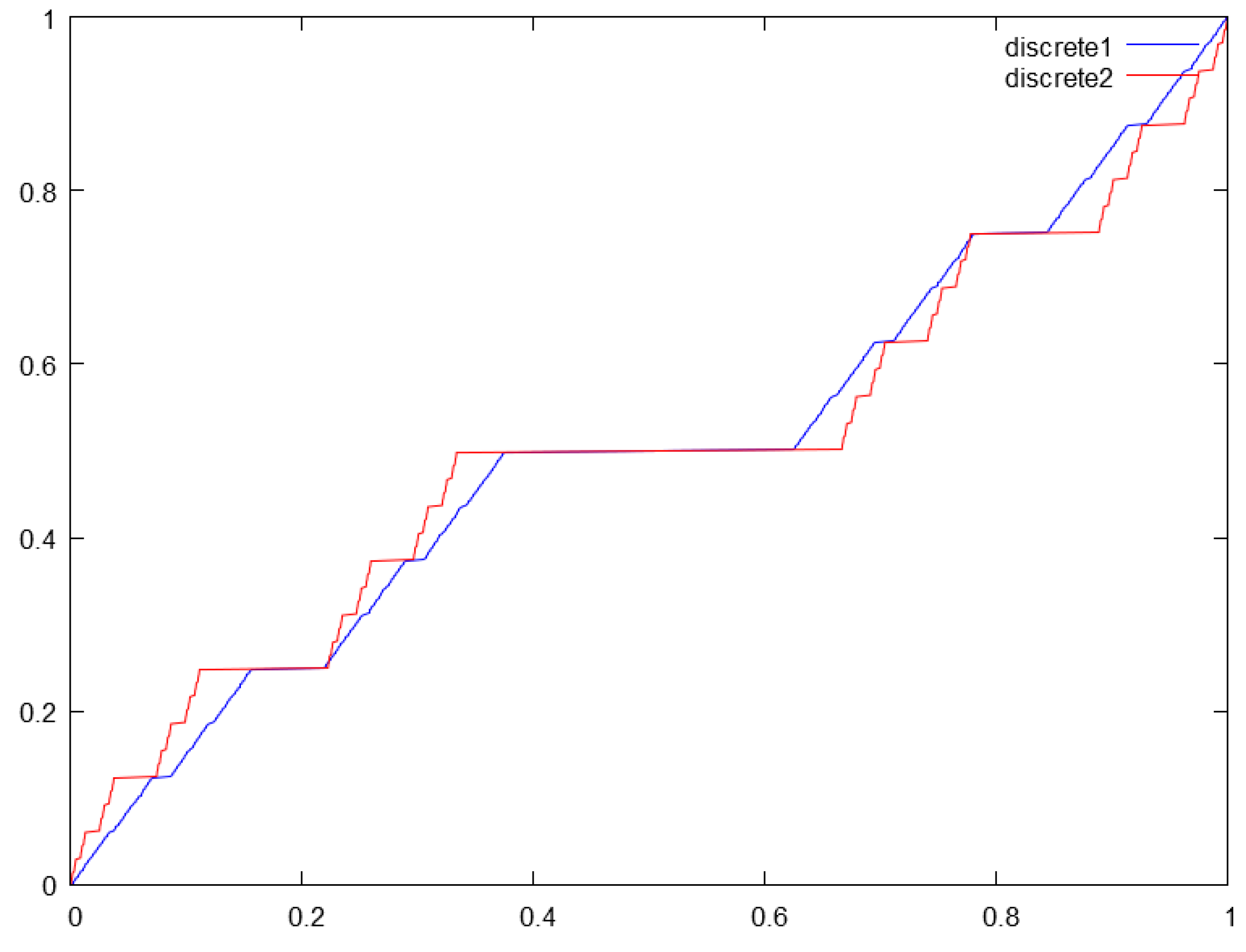
The set presented above can be used to construct a singular function, resembling by some of its properties the Cantor function described above (see Figure 2). On the other hand it is Lipschitz on its set of change.

Definition 8

(SVC Function). Define the SVC function as the map between the SVC set defined above and the dyadic rationals $D\setminus \{1/2\}$ in the following construction. Let $S_n$ be the sequence of the end-points of the interval in the n-th step in the construction of the SVC set. Let $D_n$ be the sequence of dyadic rationals with denominator $2^n$ excluding $1/2$.

Define the sequence of continuous piece-wise linear functions (see Figure 2) $F_n:[0,1]\mapsto [0,1]$, such that

$$F_n\left(S_n\right)=D_n$$

and the limit $F_C\left(x\right):=\underset{n\to \infty }{lim}{F}_n\left(x\right)$.

In the following argument we characterize the set of growth of the SVC function. In the case of the SVC function $I=[0,1]$. Then, by construction, the set $C=\{x:F_C^{\prime }\left(x\right)=0\}$ has measure $1/2$. On the other hand, for $u\in S_n$ and $h_0=1$

$$h_k=\frac{1}{2}\left(h_{k-1}-\frac{1}{4^k}\right)$$

$$q_k=2^k{h}_k=2^{k-1}{h}_{k-1}-\frac{1}{2^{k+1}}=q_{k-1}-\frac{1}{2^{k+1}}$$

Then by induction

$$q_n=1-\frac{1}{2}\sum _{k=1}^n\frac{1}{2^k}$$

Therefore, in limit

$$q^{*}=1-\frac{1}{2}\left(\frac{1}{1-1/2}-1\right)=\frac{1}{2}$$

Then for the difference quotient

$$\frac{{\Delta }_{h_n}{F}_n\left(u\right)}{h_n}=\frac{1}{q_n}$$

Therefore, in limit

$$\underset{n\to \infty }{lim}\frac{{\Delta }_h{F}_n\left(u\right)}{h}=F_C^{\prime -}\left(u\right)=2$$

while $F_C^{\prime +}\left(u\right)=0$. Therefore, $|\Delta [F_C^{\prime \pm }\left]\right|=1/2$.

Theorem 3.

Let S denote the SVC set and $I=[0,1]$. Then $F_C^{\prime +}\left(u\right)=0$ on $u\in I\setminus S$ and $F_C^{\prime -}\left(u\right)=2$ on $u\in S$. Moreover, $|F_C^{\prime \pm }\left(u\right)=0|=1/2$ and $|\Delta [F_C^{\prime \pm }\left]\right|=1/2$.

The last result demands that the hypothesis of the Lebesgue’s monotone differentiation theorem requires strict monotonicity of the function.

References

- Carpinteri, A.; Cornetti, P. A fractional calculus approach to the description of stress and strain localization in fractal media. Chaos Solitons Fractals 2002, 13, 85–94. [Google Scholar] [CrossRef]
- Carpinteri, A.; Chiaia, B.; Cornetti, P. A fractal theory for the mechanics of elastic materials. Mater. Sci. Eng. 2004, 365, 235–240. [Google Scholar] [CrossRef]
- Carpinteri, A.; Cornetti, P.; Sapora, A.; Paola, M.D.; Zingales, M. Fractional calculus in solid mechanics: Local versus non-local approach. Phys. Scr. 2009, T136, 014003. [Google Scholar] [CrossRef]
- Balankin, A.S.; Elizarraraz, B.E. Map of fluid flow in fractal porous medium into fractal continuum flow. Phys. Rev. 2012, 85. [Google Scholar] [CrossRef] [PubMed]
- Fleron, J.F. A Note on the History of the Cantor Set and Cantor Function. Math. Mag. 1994, 67, 136–140. [Google Scholar] [CrossRef]
- Dovgoshey, O.; Martio, O.; Ryazanov, V.; Vuorinen, M. The Cantor function. Expos. Math. 2006, 24, 1–37. [Google Scholar] [CrossRef] [Green Version]
- Kairies, H.H. Functional equations for peculiar functions. Aequationes Math. 1997, 53, 207–241. [Google Scholar] [CrossRef]
- Kuczma, M.; Choczewski, B.; Ger, R. Iterative Functional Equations; Cambridge University Press: Cambridge, UK, 2003. [Google Scholar]
- Chalice, D.R. A Characterization of the Cantor Function. Am. Math. Mon. 1991, 98, 255–258. [Google Scholar] [CrossRef]
- Prodanov, D. Conditions for continuity of fractional velocity and existence of fractional Taylor expansions. Chaos Solitons Fractals 2017, 102, 236–244. [Google Scholar] [CrossRef]
- Prodanov, D. Fractional Velocity as a Tool for the Study of Non-Linear Problems. Fractal Fract. 2018, 2, 4. [Google Scholar] [CrossRef]
- Cherbit, G. Fractals, dimension non entiére et applications. In Fractals, Dimension non Entière et Applications; Masson: Paris, France, 1987; chapter Dimension locale, quantité de mouvement et trajectoire; pp. 340–352. [Google Scholar]
- Adda, F.B.; Cresson, J. About Non-differentiable functions. J. Math. Anal. Appl. 2001, 263, 721–737. [Google Scholar] [CrossRef]
- Prodanov, D. Fractional variation of Hölderian functions. Fract. Calc. Appl. Anal. 2015, 18, 580–602. [Google Scholar] [CrossRef]
- DiMartino, R.; Urbina, W.O. Excursions on Cantor-Like Sets. arXiv 2017, arXiv:1411.7110v2. [Google Scholar]
Figure 1.
Recursive construction of Cantor’s function and its bounds. is approximated by an iteration function system, iterations. (a) ; (b) .
Figure 2.
Approximations of the SVC (Smith-Volterra-Cantor) and Cantor’s functions. Blue (discrete1)—SVC function, red (discrete2)—Cantor’s function; both functions are computed for six levels of iteration.
© 2019 by the author. Licensee MDPI, Basel, Switzerland. This article is an open access article distributed under the terms and conditions of the Creative Commons Attribution (CC BY) license (http://creativecommons.org/licenses/by/4.0/).
Share and Cite
MDPI and ACS Style
Prodanov, D. Characterization of the Local Growth of Two Cantor-Type Functions. Fractal Fract. 2019, 3, 45. https://doi.org/10.3390/fractalfract3030045
AMA Style
Prodanov D. Characterization of the Local Growth of Two Cantor-Type Functions. Fractal and Fractional. 2019; 3(3):45. https://doi.org/10.3390/fractalfract3030045
Chicago/Turabian StyleProdanov, Dimiter. 2019. "Characterization of the Local Growth of Two Cantor-Type Functions" Fractal and Fractional 3, no. 3: 45. https://doi.org/10.3390/fractalfract3030045