Julia and Mandelbrot Sets for Dynamics over the Hyperbolic Numbers

Abstract

Julia and Mandelbrot sets, which characterize bounded orbits in dynamical systems over the complex numbers, are classic examples of fractal sets. We investigate the analogs of these sets for dynamical systems over the hyperbolic numbers. Hyperbolic numbers, which have the form $x+\tau y$ for $x,y\in \mathbb{R}$, and ${\tau }^2=1$ but $\tau \ne \pm 1$, are the natural number system in which to encode geometric properties of the Minkowski space ${\mathbb{R}}^{1,1}$. We show that the hyperbolic analog of the Mandelbrot set parameterizes the connectedness of hyperbolic Julia sets. We give a wall-and-chamber decomposition of the hyperbolic plane in terms of these Julia sets.

1. Introduction

The Mandelbrot set, arising from the study of dynamical systems on the complex plane, has been an object of interest ever since its introduction by Robert W. Brooks and Peter Matelski [1]. With its combination of simplicity of definition and complexity of structure, the set exhibits one of the most classical fractal patterns in mathematics.

The Mandelbrot set gives the set of complex parameter values c for which the orbit of the initial point $z_0=0$ is bounded under iterations of the map $f_c:\mathbb{C}\to \mathbb{C}$ defined by

$$\begin{array}{c}\hfill f_c(z)\doteq z^2+c.\end{array}$$

Definition 1.

The Mandelbrot set ${\mathcal{M}}_{\mathbb{C}}$ is the set of complex numbers $c\in \mathbb{C}$ for which there exists some $B_c\in \mathbb{R}$ such that for all $n\in \mathbb{N}$, the inequality $\left|f_c^n(0)\overline{f_c^n(0)}\right|<B_c$ is satisfied.

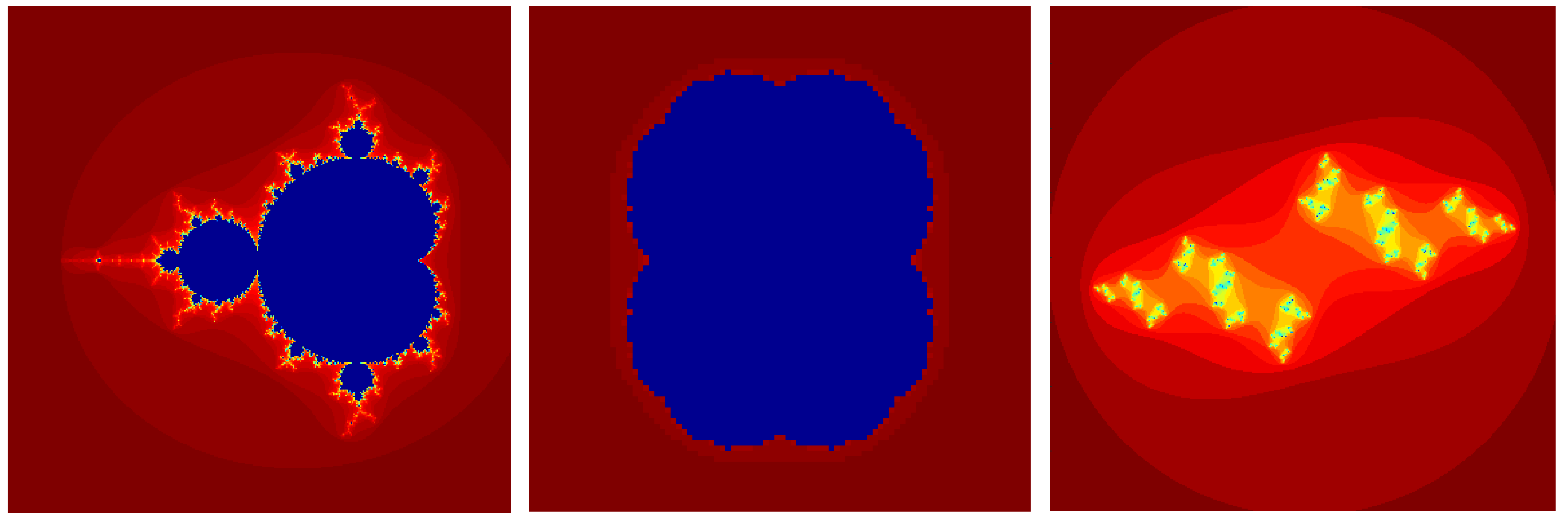
The left panel of Figure 1 shows the Mandelbrot set.

Julia sets, studied by the pioneers of complex dynamics Gaston Julia and Pierre Fatou, are subsets of complex phase space and also exhibit fractal structure.

Definition 2.

Fix a polynomial $f:\mathbb{C}\to \mathbb{C}$. The filled Julia set associated with f, denoted by ${\mathcal{K}}_{\mathbb{C}}(f)$, is the set of values $z_0\in \mathbb{C}$ for which there exists some $B_{z_0}\in \mathbb{R}$ such that for all $n\in \mathbb{N}$, the inequality $\left|f^n(z_0)\overline{f^n(z_0)}\right|<B_{z_0}$ is satisfied. The Julia set associated with f, denoted by ${\mathcal{J}}_{\mathbb{C}}(f)$, is the boundary of ${\mathcal{K}}_{\mathbb{C}}(f)$.

Julia sets associated with the complex quadratic polynomial $f_c$ that defines the Mandelbrot set are shown in the center and right panels of Figure 1. These examples illustrate a surprising connection of a topological nature between Mandelbrot and Julia sets given by the dichotomy theorem.

Dichotomy Theorem.

The Mandelbrot set parameterizes the connectedness of filled Julia sets: The filled Julia set ${\mathcal{K}}_{\mathbb{C}}(f_c)$ is connected if c is in the Mandelbrot set and totally disconnected otherwise.

For the examples of Figure 1, the choice $c=0.2$ for the center panel lies in the Mandelbrot set, and the Julia set is connected; whereas the choice $c=-1+0.5i$ for the right panel lies outside the Mandelbrot set, and the Julia set is totally disconnected. A discussion and proof of this significant result in complex dynamics may be found in [2]. The dichotomy theorem showcases the idea of viewing $\mathbb{C}$ as both the parameter space and the dynamical plane for a dynamical system.

Given the rich results for iterations of quadratic maps on the complex plane, it is natural to wonder about the behavior of dynamics on a less well-known, but also very useful sibling of the complex numbers, the hyperbolic numbers, $\mathbb{H}$ [3]. This number system has connections to diverse topics such as general relativity, differential equations, and the study of abstract algebras [4,5].

The first to explore a hyperbolic number analog to the hyperbolic numbers (under the name of perplex numbers) was Senn [6], who in 1990 performed numerical experiments revealing that the hyperbolic analog to the Mandelbrot set has a completely different character from the (complex) Mandelbrot set. For the quadratic map $f(z)=z^2+c$, for $z,c\in \mathbb{H}$, Senn’s simulations indicated that the set of values of c for which the orbit $f^n(0)$ is bounded consists of a square with one of its diagonals on the real axis between $(-2,0)$ and $(\frac{1}{4},0)$. Artzy [7] and Metzler [8] independently proved this conjecture. Artzy further showed that Julia sets for quadratic maps with the constant c in the hyperbolic Mandelbrot set are connected, rectangular sets. This suggests that the dichotomy theorem may also hold for hyperbolic quadratic maps. Artzy states that the hyperbolic Julia set is disconnected for values of c outside of the Mandelbrot set. Fishback [9] describes, with reference to Artzy [7], these disconnected hyperbolic Julia sets as being stretched Cantor sets or products of Cantor sets. Proofs or explicit descriptions of these disconnected hyperbolic Julia sets are, however, not found in [7] or [9].

In this paper, we provide explicit descriptions, with proofs, for Julia sets over $\mathbb{H}$. Hyperbolic Julia sets turn out to have one of four characteristics: they may be empty, the product of intervals, the product of a Cantor set and an interval, or the product of two Cantor sets. Our main result is a wall-and-chamber decomposition of the hyperbolic plane, which gives the regions of the parameter space that give rise to each of these types of Julia sets. This clarifies the results and statements of [7,9] by providing an explicit statement and proof of the hyperbolic-number analog to the dichotomy theorem:

Quadchotomy Theorem.

The hyperbolic Mandelbrot set parameterizes the connectedness of filled hyperbolic Julia sets.

The quadchotomy theorem is stated explicitly as Theorem 2.

Structure of the Paper

In Section 2, we provide an introduction to the hyperbolic numbers, emphasizing characteristic coordinates. Section 3 explicitly defines the hyperbolic Mandelbrot and Julia sets (slightly differently from Artzy [7] in the choice of a hyperbolic analog of boundedness). We give an explicit description of the former, mirroring the results of Artzy [7] and Metzler [8]. The main result, the quadchotomy theorem, is proven in Section 4.

2. Hyperbolic Numbers

The hyperbolic numbers $\mathbb{H}$, sometimes called perplex numbers, motor variables, split-complex numbers, Lorentz numbers, Minkowski numbers, or a variety of other names, can be understood in several contexts [3,4,5,10]. Algebraically, $\mathbb{H}$ can be identified with the ring $\mathbb{R}[t]/(t^2-1)$, where we call $\tau$ the image of t in the quotient. Hence, they are abstractly isomorphic to $\mathbb{R}\oplus \mathbb{R}$ as a module over $\mathbb{R}$, with generators 1 and $\tau$. In analogy to the complex numbers, we write $z=u+\tau v$ for $u,v\in \mathbb{R}$, where ${\tau }^2=1$, but $\tau \ne \pm 1$.

Seen as a module over $\mathbb{R}$, hyperbolic numbers admit an automorphism, which acts trivially on the component generated by 1, called hyperbolic conjugation. If $z=x+\tau y$, the hyperbolic conjugate is $\overline{z}=x-\tau y$. Hyperbolic conjugation shares properties with complex conjugation; $z=\overline{\overline{z}}$, $\overline{z}+\overline{w}=\overline{z+w}$, and $\overline{z}\overline{w}=\overline{zw}$.

We will refer to $\mathbb{H}$ as the hyperbolic plane in analogy to the complex plane; our usage is entirely distinct from the geometric notion of the plane equipped with a hyperbolic metric, which would typically be modeled with the Poincaré disk or upper half plane. Indeed, the hyperbolic numbers are equipped with a quadratic form, but it does not give rise to a metric or norm. Instead, if $z=x+\tau y$,

$$\begin{array}{c}\hfill \left|\right|z\left|\right|=z\overline{z}=x^2-y^2.\end{array}$$

Representing the hyperbolic number $z=x+\tau y$ as the matrix:

$$z=\left[\begin{array}{cc}x& y\\ y& x\end{array}\right]=\left[\begin{array}{cc}1& 1\\ -1& 1\end{array}\right]\left[\begin{array}{cc}x-y& 0\\ 0& x+y\end{array}\right]{\left[\begin{array}{cc}1& 1\\ -1& 1\end{array}\right]}^{-1},$$

and addition $z_1+z_2=(x_1+\tau y_1)+(x_2+\tau y_2)=(x_1+x_2)+j(y_1+y_2)$ and multiplication $z_1{z}_2=(x_1+\tau y_1)(x_2+\tau y_2)=(x_1{x}_2+y_1{y}_2)+\tau (x_1{y}_2+x_2{y}_1)$ correspond respectively to matrix addition and multiplication. The matrix approach reveals the natural characteristic coordinates $X=x-y$ and $Y=x+y$ with which to work with hyperbolic numbers, as noted by Fishback [9]. Representing a hyperbolic number in characteristic coordinates as

$$z=\left(\begin{array}{cc}X& 0\\ 0& Y\end{array}\right),$$

the hyperbolic multiplication

$$z_1{z}_2=\left[\begin{array}{cc}{x}_1& y_1\\ y_1& x_1\end{array}\right]\left[\begin{array}{cc}{x}_2& y_2\\ y_2& x_2\end{array}\right]=\left[\begin{array}{cc}{x}_1{x}_2+y_1{y}_2& x_1{y}_2+x_2{y}_1\\ x_1{y}_2+x_2{y}_1& x_1{x}_2+y_1{y}_2\end{array}\right]$$

is simply

$$z_1{z}_2=\left(\begin{array}{cc}{X}_1& 0\\ 0& Y_1\end{array}\right)\left(\begin{array}{cc}{X}_2& 0\\ 0& Y_2\end{array}\right)=\left(\begin{array}{cc}{X}_1{X}_2& 0\\ 0& Y_1{Y}_2\end{array}\right).$$

In addition, the quadratic form has a simple form in characteristic coordinates:

$$\begin{array}{c}\hfill z\overline{z}=(x+\tau y)(x-\tau y)=x^2-y^2=(x-y)(x+y)=XY.\end{array}$$

(1)

The sets $D_{+}:=\{z=x+\tau x\}$ and $D_{-}:=\{z=x-\tau x\}$ in the hyperbolic plane where either characteristic coordinate vanishes form the axes of the characteristic coordinate system. Note that $D_{+}$ and $D_{-}$ are closed under addition and multiplication.

3. The Hyperbolic Mandelbrot Set

The simple representation of multiplication for hyperbolic numbers in characteristic coordinates gives rise to hyperbolic Mandelbrot and Julia sets that contrast significantly with the classical Mandelbrot and Julia sets of complex numbers. Our definitions for hyperbolic Mandelbrot and Julia sets closely follow the corresponding definitions over $\mathbb{C}$. If $f:\mathbb{H}\to \mathbb{H}$ is a function, we again write $f^2(z):=f(f(z))$, $f^3(z):=f(f(f(z)))$, etc.

Definition 3.

For each $c\in \mathbb{H}$, consider the map

$$\begin{array}{c}\hfill f_c(z)=z^2+c.\end{array}$$

The hyperbolic Mandelbrot set ${\mathcal{M}}_{\mathbb{H}}$ is the set of values $c\in \mathbb{H}$ for which there exists some $B_c\in \mathbb{R}$ such that for all $n\in \mathbb{N}$, the inequality $\left|f_c^n(0)\overline{f_c^n(0)}\right|<B_c$ is satisfied.

Definition 4.

Fix a polynomial $f(z):\mathbb{H}\to \mathbb{H}$. The hyperbolic filled Julia set associated with f, denoted by ${\mathcal{K}}_{\mathbb{H}}(f)$, is the set of values $z_0\in \mathbb{H}$ for which there exists some $B_{z_0}\in \mathbb{R}$ such that for all $n\in \mathbb{N}$, the inequality $\left|f^n(z_0)\overline{f^n(z_0)}\right|<B_{z_0}$ is satisfied. The hyperbolic Julia set associated with f, denoted by ${\mathcal{J}}_{\mathbb{H}}(f)$, is the boundary of ${\mathcal{K}}_{\mathbb{H}}(f)$.

The quantity $\left|f^n(z_0)\overline{f^n(z_0)}\right|$ is equal to zero on the characteristic axes $D_{\pm }$, and therefore, the bound $\left|f^n(z_0)\overline{f^n(z_0)}\right|<B_{z_0}$ automatically holds on these sets even though the real and hyperbolic components of $f^n(z_0)$ may be limited to infinity. Artzy [7] makes a different choice in the definition of the hyperbolic Julia set in that he bounds the real and hyperbolic parts.

The similarities in definition to the complex case lead to several of the same immediate results. We will use the fact that, as for the complex Mandelbrot set [2], ${\mathcal{M}}_{\mathbb{H}}$ is invariant under conjugation. We note as well that since both complex and hyperbolic conjugations fix $\mathbb{R}\subset \mathbb{C},\mathbb{H}$, we must have ${\mathcal{M}}_{\mathbb{H}}\cap \mathbb{R}={\mathcal{M}}_{\mathbb{C}}\cap \mathbb{R}$.

Remark 1.

The two definitions are in many ways similar, but the Mandelbrot set is a subset of parameter space, whereas a Julia set is said to lie in the dynamical plane. Theorem 2 makes the connection between ${\mathcal{M}}_{\mathbb{H}}$ and ${\mathcal{K}}_{\mathbb{H}}(f)$ explicit for f quadratic.

Key to determining the hyperbolic Mandelbrot and Julia sets is the observation that in characteristic coordinates, the map $f_c(z)=z^2+c_1+\tau c_2$ decouples into the real quadratic map $f_c(x)=x^2+c$ on each coordinate. Indeed, $f_c$ can be written as

$$\begin{array}{cc}\hfill f_c(x,y)& =(x^2+y^2+c_1,2xy+c_2)\hfill \\ & =\left(\frac{1}{2}\left(X^2+Y^2\right)+c_1,\frac{1}{2}\left(Y^2-X^2\right)+c_2\right);\hfill \end{array}$$

or, writing $f_c$ as a function characteristic coordinates,

$$\begin{array}{cc}\hfill f_c(X,Y)& =\left(X^2+c_1-c_2,Y^2+c_1+c_2\right)\hfill \\ & =\left(X^2+c_X,Y^2+c_Y\right)\hfill \\ & =\left(f_{c_X}(X),f_{c_Y}(Y)\right),\hfill \end{array}$$

(2)

where $c_X=c_1-c_2$ and $c_Y=c_1+c_2$ are representations of the constants in characteristic coordinates. In characteristic coordinates, the map decouples into a map on each coordinate, so that under iteration, we have

$$\begin{array}{c}\hfill f_c^n(X,Y)=\left(f_{c_X}^n(X),f_{c_Y}^n(Y)\right).\end{array}$$

(3)

The map $f_c(x)=x^2+c:\mathbb{R}\to \mathbb{R}$ (for $x,c\in \mathbb{R}$), whose behavior is well known [2], is therefore key to finding hyperbolic Julia sets.

For $c\le \frac{1}{4}$, the behavior of the dynamical system $x_{n+1}=f_c(x_n)$ may be understood by a change of coordinates to the well-known logistic map. Writing

$${\rho }_{+}(c)=\frac{1+\sqrt{1-4c}}{2},\xi =\frac{1}{2}\left(1-\frac{x}{{\rho }_{+}(c)}\right),r=2{\rho }_{+}(c),$$

the dynamical system $x_{n+1}=f_c(x_n)$ becomes the logistic dynamical system ${\xi }_{n+1}=g_r({\xi }_n)$ for $g_r(\xi )=r(1-\xi )\xi$.

The case $c<-2$ corresponds to $r>4$, for which all orbits of the logistic map diverge to infinity except for points in a Cantor set. For $g_r(\xi )$, the Cantor set is contained in $[0,{\eta }_{-}]\cup [{\eta }_{+},1]$, where ${\eta }_{\pm }=\frac{1}{2r}(r\pm \sqrt{r^2-4r})$. For $f_c(x)$, this translates to a Cantor set contained in $[-{\rho }_{+}(c),-\gamma (c)]\cup [\gamma (c),{\rho }_{+}(c)]$, where $4{\gamma }^2(c)=-4c-2-2\sqrt{1-4c}$. Note that for $c<-2$, $\gamma (c)<0$, so the Cantor set for $f_c(x)$ is bounded away from zero.

The case $-2\le c\le \frac{1}{4}$ corresponds to $1\le r\le 4$, for which orbits of the logistic map are bounded for $\xi \in [0,1]$ and diverge to infinity otherwise. That is, for $c\in [-2,\frac{1}{4}]$, the orbit $f_c^n(x)$ is bounded if and only if $-{\rho }_{+}(c)\le x\le {\rho }_{+}(c)$. In this case, the fixed points are $x=\frac{1}{2}(1\pm \sqrt{1-4c})$; there is a fixed point equal to zero only for $c=0$.

That ${\mathcal{K}}_{\mathbb{C}}(f_c)\cap \mathbb{R}$ is empty for $\frac{1}{4}<c$ may be seen as follows: For any $x\in \mathbb{R}$, the minimum value of $f_c(x)-x$ is $c-\frac{1}{4}$. Thus, for any $x_0\in \mathbb{R}$ and positive integer n, $f_c^{n+1}(x_0)\ge f_c^n(x_0)+c-\frac{1}{4}$; $f_c^n(x_0)\ge x_0+n\left(c-\frac{1}{4}\right)$. It follows that for $c>\frac{1}{4}$, $f_c^n(x_0)\to \infty$ as $n\to \infty$.

In summary, we have the following:

Lemma 1.

Let $f_c(z)=z^2+c$ for $c\in \mathbb{R}$. Then, the intersection ${\mathcal{K}}_{\mathbb{C}}(f_c)\cap \mathbb{R}$ is

(i) 

a Cantor set not containing zero if $c<-2$,

(ii) 

the interval $-{\rho }_{+}(c)\le x\le {\rho }_{+}(c)$ if $-2<c<\frac{1}{4}$,

(iii) 

empty if $\frac{1}{4}<c$.

The decoupling of the characteristic coordinates endows ${\mathcal{M}}_{\mathbb{H}}$ with a much simpler structure than ${\mathcal{M}}_{\mathbb{C}}$, as detailed in the next theorem, due to Artzy and Metzler [7,8].

Theorem 1.

Let S be the square given by

$$\begin{array}{cc}\hfill S:& =\left\{max\left(x-\frac{1}{4},-x-2\right)\le y\le min\left(x+2,-x+\frac{1}{4}\right)\right\}\hfill \\ & =\left\{(X,Y)\in {\left[-2,\frac{1}{4}\right]}^2\right\},\hfill \end{array}$$

and let $D=D_{+}\cup D_{-}$ be the union of the diagonals in $\mathbb{H}$. Then, ${\mathcal{M}}_{\mathbb{H}}=S\cup D$.

Proof. 

We need to determine the values of c for which $|f_c^n(0=0+0\tau )|$ is bounded as n approaches infinity. The expression (3) for iterates of the map $f_c(z)$ in characteristic coordinates allows us to write $|f_c^n(0)|=|f_{c_X}^n(0)f_{c_Y}^n(0)|.$ According to Lemma 1, $f_{c_{X,Y}}^n(0)$ are bounded for (and only for) $-2\le c_{X,Y}\le \frac{1}{4}$. Thus, $|f_c^n(0)|$ is bounded for $(c_X,c_Y)\in S=\left\{(X,Y)\in {\left[-2,\frac{1}{4}\right]}^2\right\}$.

It could also be the case that, without loss of generality, $f_{c_X}^n(0)\to 0$, but $f_{c_Y}^n(0)\to \infty$ in a manner so that their product is bounded. Since $f_{c_X}^n(0)\to 0$ only for $c_X=0$, such cases occur only for $(c_X,c_Y)$ on the union D. D is, in fact, in ${\mathcal{M}}_{\mathbb{H}}$: Since $D_{+}$ and $D_{-}$ are closed under addition and multiplication, the restrictions $f_c{|}_{D_{\pm }}:D_{\pm }\to D_{\pm }$ are well defined. However, since $\left|z\overline{z}\right|=0$ for all $z\in D$, we have that $D\subset {\mathcal{M}}_{\mathbb{H}}$. □

The center panel of Figure 2 depicts the hyperbolic Mandelbrot set.

Remark 2.

As implied by Theorem 2 below, the fact that the part of D outside of S is in the Mandelbrot set is largely an artifact of the fact that $D_{+}$ and $D_{-}$ are ideals of $\mathbb{H}$.

4. Hyperbolic Julia Sets

Over the complex numbers, ${\mathcal{M}}_{\mathbb{C}}$ determines the points in parameter space that correspond to connected Julia sets. One may ask if ${\mathcal{M}}_{\mathbb{H}}$ performs the analogous role for the hyperbolic numbers. The positive answer may be given more nuance, as $\mathbb{H}$ as a parameter space admits a wall-and-chamber decomposition based on the form of ${\mathcal{K}}_{\mathbb{H}}(f)$, in which ${\mathcal{M}}_{\mathbb{H}}$ is the chamber corresponding to connectedness of nonempty filled Julia sets. We now develop this decomposition explicitly.

Proposition 1.

For $c\in \mathbb{H}$, let $c=(c_X,c_Y)$ be its description in characteristic coordinates, and let $f_c(z)=z^2+c$. Write $f_{c_X}(X)=X^2+c_X$ and $f_{c_Y}(Y)=Y^2+c_Y$. For $c_X,c_Y\ne 0$, the filled hyperbolic Julia set ${\mathcal{K}}_{\mathbb{H}}(f_c)$ is equal to the Cartesian product of ${\mathcal{K}}_{\mathbb{C}}(f_{c_X})\cap \mathbb{R}$ and ${\mathcal{K}}_{\mathbb{C}}(f_{c_Y})\cap \mathbb{R}$.

Proof. 

Let $z_0=(X_0,Y_0)$ in characteristic coordinates. By equation $(1)$, $\left|f^n(z_0)\overline{f^n(z_0)}\right|=\left|f_{c_X}^n(X_0)f_{c_Y}^n(Y_0)\right|$ = $\left|f_{c_X}^n(X_0)\right|\left|f_{c_Y}^n(Y_0)\right|$. According to the discussion leading to Lemma 1, ${lim}_{n\to \infty }{f}_c^n(X_0)=0$ only for $c=0$. For $c_X,c_Y\ne 0$, there is a $B_{z_0}$ such that $\left|f_{c_X}^n(X_0)f_{c_Y}^n(Y_0)\right|<B_{z_0}$ for all n if and only if there is some $M_{z_0}\in \mathbb{R}$ such that for all n $\left|f_{c_X}^n(X_0)\right|$, $\left|f_{c_Y}^n(Y_0)\right|<M_{z_o}$. However, since $c_X,X_0\in \mathbb{R}$, we have $\left|f_{c_X}^n(X_0)\right|<M_{z_0}$ if and only if $X_0\in {\mathcal{K}}_{\mathbb{C}}(f_{c_X})\cap \mathbb{R}$, $Y_0\in {\mathcal{K}}_{\mathbb{C}}(f_{c_Y})\cap \mathbb{R}$. We conclude that, for $c_X,c_Y\ne 0$,

$$\begin{array}{c}\hfill {\mathcal{K}}_{\mathbb{H}}(f_c)=\left\{(X,Y):|f_{c,X}^n(X)·f_{c,Y}^n(Y)|<B_{z_0}\right\}=\left\{{\mathcal{K}}_{\mathbb{C}}(f_{c_X})\cap \mathbb{R}\right\}\times \left\{{\mathcal{K}}_{\mathbb{C}}(f_{c_Y})\cap \mathbb{R}\right\}.\end{array}$$

□

Examples of filled hyperbolic Julia sets are shown in the side panels of Figure 2. The filled hyperbolic Julia sets may be totally disconnected (Panel A), connected but not totally disconnected (Panel B), connected and nonempty (Panel C), or empty (Panel D). These examples represent the decomposition of $\mathbb{H}$ stated in the following analog to the dichotomy theorem of complex Mandelbrot and filled Julia sets and depicted in Figure 3:

Theorem 2 (Quadchotomy).

For $c\in \mathbb{H}$, let $f_c(z)=z^2+c$, and let $c=(c_X,c_Y)$ in characteristic coordinates, with $c_X,c_Y\ne 0$. Then, $\mathbb{H}$ admits a wall-and-chamber decomposition as follows:

(i) 

if $c\in S$, then ${\mathcal{K}}_{\mathbb{H}}(f_c)$ is nonempty and connected;

(ii) 

if one of $c_X,c_Y$ is in $[-2,\frac{1}{4}]$ and the other is less than or equal to $-2$, then ${\mathcal{K}}_{\mathbb{C}}(f_c)$ is disconnected;

(iii) 

if $c_X,c_Y<-2$, then ${\mathcal{K}}_{\mathbb{C}}(f_c)$ is totally disconnected;

(iv) 

otherwise, ${\mathcal{K}}_{\mathbb{H}}(f_c)$ is empty.

Proof. 

By Proposition 1, we need to understand ${\mathcal{K}}_{\mathbb{C}}(f_{c_X})\cap \mathbb{R}$ and ${\mathcal{K}}_{\mathbb{C}}(f_{c_Y})\cap \mathbb{R}$, which are given in Lemma 1.

Part (i): When $c\in S$, $c_X,c_Y\in [-2,\frac{1}{4}]$, and ${\mathcal{K}}_{\mathbb{C}}(f_{c_X})$ and ${\mathcal{K}}_{\mathbb{C}}(f_{c_Y})$ are both simply connected and conjugate-invariant. Thus, ${\mathcal{K}}_{\mathbb{C}}(f_{c_X})\cap \mathbb{R}$ and ${\mathcal{K}}_{\mathbb{C}}(f_{c_Y})\cap \mathbb{R}$ are both connected, so ${\mathcal{K}}_{\mathbb{H}}(f_c)$ is as well.

Part (ii): In this case, exactly one of ${\mathcal{K}}_{\mathbb{C}}(f_{c_X})\cap \mathbb{R}$ or ${\mathcal{K}}_{\mathbb{C}}(f_{c_Y})\cap \mathbb{R}$ is connected; the other is a Cantor set. The product of a Cantor set and a connected set is a disconnected set.

Part (iii): Both ${\mathcal{K}}_{\mathbb{C}}(f_{c_X})\cap \mathbb{R}$ and ${\mathcal{K}}_{\mathbb{C}}(f_{c_Y})\cap \mathbb{R}$ are Cantor sets, which are totally disconnected, and the product of two totally disconnected sets is again totally disconnected.

Part (iv): By Lemma 1, at least one of ${\mathcal{K}}_{\mathbb{C}}(f_{c_X})\cap \mathbb{R}$ or ${\mathcal{K}}_{\mathbb{C}}(f_{c_Y})\cap \mathbb{R}$ is empty, so their product is as well. □

We ignored the characteristic axes in Theorem 2. We compute their Julia sets as follows: If, say, $c_Y=0$, then $\left|f_c^n(z_0)\overline{f_c^n(z_0)}\right|=\left|f_{c_X}^n(X_0)f_{c_Y}^n(Y_0)\right|=Y_0^{2n}\left|f_{c_X}^n(X_0)\right|$. The ratio of $\left|f^{n+1}(z_0)\overline{f^{n+1}(z_0)}\right|$ to $\left|f^n(z_0)\overline{f^n(z_0)}\right|$ is $Y_0^2\frac{\left|f_{c_X}^{n+1}(X_0)\right|}{\left|f_{c_X}^n(X_0)\right|}=Y_0^2\frac{\left|f_{c_X}\left(f_{c_X}^n(X_0)\right)\right|}{\left|f_{c_X}^n(X_0)\right|}=Y_0^{2}R\left(f_{c_X}^n(X_0)\right)$, for $R(x)=x+\frac{c_X}{x}.$ If $\left|f_{c_X}^n(X_0)\right|$ is unbounded, then so is this ratio since $R(x)$ approaches infinity with x. That is, for $c_X>\frac{1}{4}$, the filled Julia set is empty. For $c_X<\frac{1}{4}$, the Julia set is the product $(X_0,Y_0)\in \mathfrak{C}\times [-1,1]$ for a Cantor set $\mathfrak{C}$ contained in $[-{\rho }_{+}(c_X),-\gamma (c_X)]\cup [\gamma (c_X),{\rho }_{+}(c_X)]$.

5. Discussion

The decoupling into characteristic coordinates allows for the computation of Mandelbrot and Julia sets for hyperbolic numbers. These sets are simpler than their counterparts in the complex number setting. However, an analog to the dichotomy theorem for complex dynamics carries over to hyperbolic dynamics.

Complex numbers and hyperbolic numbers are two of the three classes of what are called binary numbers. Senn [6] also numerically investigated the third class of binary numbers, namely parabolic numbers $z=a+bϵ$, where ${ϵ}^2=0$. Fishback [9] found the Mandelbrot set of these numbers, which form what is called the Laguerre plane. Fishback and Horton further showed that an analog of the dichotomy theorem extends to three-component number systems, the ternary numbers [11].

Binary numbers are two-dimensional examples of Clifford algebras. Do analogs of the dichotomy theorem also hold for higher dimensional Clifford algebras, such as quaternions, octonions, and their hyperbolic counterparts?