Stokes’ First Problem for Viscoelastic Fluids with a Fractional Maxwell Model

Abstract

Stokes’ first problem for a class of viscoelastic fluids with the generalized fractional Maxwell constitutive model is considered. The constitutive equation is obtained from the classical Maxwell stress–strain relation by substituting the first-order derivatives of stress and strain by derivatives of non-integer orders in the interval $(0,1]$. Explicit integral representation of the solution is derived and some of its characteristics are discussed: non-negativity and monotonicity, asymptotic behavior, analyticity, finite/infinite propagation speed, and absence of wave front. To illustrate analytical findings, numerical results for different values of the parameters are presented.

1. Introduction

Viscoelastic fluid flows with the classical Maxwell constitutive model [1] have been the object of intense study for many years, for a short survey see for example [2,3]. In the case of a unidirectional flow, the Maxwell constitutive relation has the dimensionless form

$$\sigma +a\frac{\partial \sigma }{\partial t}=b\frac{\partial \epsilon }{\partial t},$$

(1)

where $\sigma$ and $\epsilon$ are shear stress and strain, respectively, a is the relaxation time, and b the dynamic viscosity.

Fractional calculus, in view of its ability to model hereditary phenomena with long memory, has proved to be a valuable tool to handle viscoelastic aspects [4]. For instance, rheological constitutive equations with fractional derivatives play an important role in the description of properties of polymer solutions and melts [5]. A four-parameter generalization of the classical Maxwell model (1) has been proposed in [6], see also [7,8] and [9] (Chapter 7). It is obtained from (1) by substituting the first order time-derivatives of stress and strain with Riemann-Liouville fractional derivatives in time, which leads to the following generalized fractional Maxwell constitutive equation

$$\sigma +a{D}_t^{\alpha }\sigma =b{D}_t^{\beta }\epsilon ,$$

(2)

where $0<\alpha ,\beta \le 1$ and $a,b>0$. Since for $\alpha >\beta$, the corresponding relaxation function is increasing, which is not physically acceptable, the constitutive model (2) is considered only for fractional order parameters satisfying the constraints (see [6,7,8,9])

$$0<\alpha \le \beta \le 1,a,b>0.$$

(3)

The fractional Maxwell constitutive Equation (2) with thermodynamic constraints (3) has been shown to be an excellent model for capturing the linear viscoelastic behavior of soft materials exhibiting one or more broad regions of power-law-like relaxation [8,10,11].

Stokes’ first problem is one of the basic problems for simple flows. It is concerned with the shear flow of a fluid occupying a semi-infinite region bounded by a plate which undergoes a step increase of velocity from rest. One of the first studies on Stokes’ first problem for viscoelastic fluids is [12]. Since then many works have been devoted to this problem for different types of fluids with linear constitutive equations. Stokes’ first problem for viscoelastic fluids with general stress–strain relation is studied in [13], [14] (Section 5.4) and [4] (Chapter 4). For some recent results concerning unidirectional flows of viscoelastic fluids with fractional derivative models we refer to [15] (Chapter 7). Let us note that the fractional order governing equations are usually derived from classical models by substituting the integer order derivatives by fractional derivatives. The problem of correct fractionalization of the governing equations is discussed in [16].

The classical Maxwell constitutive Equation (1) and its fractional order generalization (2) are among the simplest viscoelastic models for fluid-like behavior and the corresponding Stokes’ first problem is a good model of essential processes involved in wave propagation. For studies on Stokes’ first problem for classical Maxwell fluids we refer to [2,3] and the references cited therein. Stokes’ first problem for generalized fractional Maxwell fluids is studied in [17,18], where explicit solutions in the form of series expansions are obtained (in [18] only the particular case $\beta =1$ is considered). Explicit solutions of other types of problems for unidirectional flows of fractional Maxwell fluids with constitutive Equation (2) can be found in [19,20,21].

Despite the abundance of works devoted to exact solutions of unidirectional flows of linear viscoelastic fluids, to the best of our knowledge, there is very little analytical work enlightening the basic properties of solution to Stokes’ first problem for fractional Maxwell fluids, such as propagation speed, non-negativity, monotonicity, regularity, and asymptotic behavior. In addition, it was pointed out in [22,23] that in a number of recent works the obtained exact solutions to Stokes’ first problem for non-Newtonian fluids contain mistakes. In the present work we provide a new explicit solution to Stokes’ first problem for generalized Maxwell fluids with a constitutive model (2) and compare it numerically to the one given in [17]. Moreover, based on the theory of Bernstein functions, we study analytically the properties of the solution and support the analytical findings by numerical results.

This paper is organized as follows. In Section 2, the material functions of the fractional Maxwell model are studied. In Section 3, the solution to Stokes’ first problem is studied analytically based on its representation in Laplace domain. Section 4 is devoted to derivation of explicit integral representation of solution and numerical computation. Some facts concerning Bernstein functions and related classes of functions are summarized in an Appendix.

2. Fractional Maxwell Model-Material Functions

Consider a unidirectional viscoelastic flow and suppose it is quiescent for all times prior to some starting time that we assume as $t=0$. Since we work only with causal functions ($f\left(t\right)=0$ for $t<0$), if there is no danger of confusion for the sake of brevity, we still denote by $f\left(t\right)$ the function $H\left(t\right)f\left(t\right)$, where $H\left(t\right)$ is the Heaviside unit step function. We are concerned with the fractional Maxwell model, given by the linear constitutive Equation (2) with parameters satisfying (3). The material functions—relaxation function $G\left(t\right)$ and the creep compliance $J\left(t\right)$—in a one-dimensional linear viscoelastic model are defined by the identities [4,24]

$$\sigma (x,t)={\int }_0^{t}G(t-\tau )\dot{\epsilon }(x,\tau )\mathrm{d}\tau ;\epsilon (x,t)={\int }_0^{t}J(t-\tau )\dot{\sigma }(x,\tau )\mathrm{d}\tau ,t>0,$$

(4)

where the over-dot denotes the first derivative in time.

Applying (A4), we derive from the constitutive Equation (2) expressions for material functions in the Laplace domain:

$$\widehat{G}\left(s\right)=\frac{b{s}^{\beta -1}}{1+a{s}^{\alpha }},\widehat{J}\left(s\right)=\frac{1}{b{s}^{\beta +1}}+\frac{a}{b{s}^{\beta -\alpha +1}}.$$

(5)

Taking the inverse Laplace transform of the above representations of $\widehat{G}\left(s\right)$ and $\widehat{J}\left(s\right)$, we get, by using the properties (A5) and (A8), the following representations of the material functions (see also [6,7,8,9])

$$G\left(t\right)=\frac{b}{a}{t}^{\alpha -\beta }{E}_{\alpha ,\alpha -\beta +1}\left(-\frac{1}{a}{t}^{\alpha }\right),J\left(t\right)=\frac{t^{\beta }}{b\Gamma (1+\beta )}+\frac{a{t}^{\beta -\alpha }}{b\Gamma (1+\beta -\alpha )},t>0,$$

(6)

in terms of the Mittag-Leffler function (A6) and power-law type functions, respectively.

The second law of thermodynamics, stating that the total entropy can only increase over time for an isolated system, implies the following restrictions on the material functions: $G\left(t\right)$ should be non-increasing and $J\left(t\right)$ non-decreasing for $t>0$. This behavior is related to the physical phenomena of stress relaxation and strain creep [4]. It has been proven that the fractional Maxwell model (2) is consistent with the second law of thermodynamics if and only if $0<\alpha \le \beta \le 1$ [6,7,8,9]. For completeness, here we formulate and prove a slightly stronger statement. In fact, it appears that the monotonicity of the material functions of the fractional Maxwell model imply that the relaxation function $G\left(t\right)$ is completely monotone and the creep compliance $J\left(t\right)$ is a complete Bernstein function. The definitions and properties of completely monotone functions and related classes of functions are summarized in the Appendix.

Proposition 1.

Assume $0<\alpha ,\beta \le 1$, $a,b>0$, $t>0$. The following assertions are equivalent:

(a) 

$0<\alpha \le \beta \le 1$;

(b) 

$G\left(t\right)$ is monotonically non-increasing for $t>0$;

(c) 

$J\left(t\right)$ is monotonically non-decreasing for $t>0$;

(d) 

$G\left(t\right)$ is a completely monotone function;

(e) 

$J\left(t\right)$ is a complete Bernstein function.

Proof. 

Using the representations (6) for the material functions, we prove that condition (a) is equivalent to any of the conditions (b)–(e). First we show that if $1\ge \alpha >\beta >0$ then (b) and (c) are not satisfied. The definition of Mittag-Leffler function (A6) implies $G\left(t\right)\sim t^{\alpha -\beta }$ for $t\to 0$. Therefore, if $\alpha >\beta$, $G\left(t\right)$ is increasing near 0, i.e., (b) is violated. Further, $\mathrm{d}J/\mathrm{d}t\sim t^{\beta -\alpha -1}/\Gamma (\beta -\alpha )$ for $t\to 0$. Since $\Gamma (\beta -\alpha )<0$ for $1\ge \alpha >\beta >0$, in this case $J\left(t\right)$ is decreasing near 0, and thus (c) is violated. Therefore, any of conditions (b) and (c) implies (a). It remains to prove that (a) implies (d) and (e), i.e., $G\left(t\right)\in \mathcal{CMF}$ and $J\left(t\right)\in \mathcal{CBF}$. Indeed, if $0<\alpha \le \beta \le 1$ then $t^{\alpha -\beta }\in \mathcal{CMF}$ and $E_{\alpha ,\alpha -\beta +1}\left(-\frac{1}{a}{t}^{\alpha }\right)\in \mathcal{CMF}$ as a composition of the completely monotone Mittag-Leffler function of negative argument and the Bernstein function $t^{\alpha }$. Therefore, $G\left(t\right)\in \mathcal{CMF}$ is a product of two completely monotone functions. The fact that $J\left(t\right)$ is a complete Bernstein function follows from the property of the power function $t^{\gamma }\in \mathcal{CBF}$ for $\gamma \in [0,1]$. ☐

Representations (6) together with the asymptotic expansion (A7) gives $G(+\infty )=0$ and $J(+\infty )=+\infty$. Therefore, the fractional Maxwell constitutive equation indeed models fluid-like behavior (for a discussion on the general conditions see e.g., [24], Section 2). More precisely, (6) and (A7) imply for $t\to +\infty$ that $G\left(t\right)\sim t^{-\alpha }$ if $\beta <1$ and $G\left(t\right)\sim t^{-\alpha -1}$ if $\beta =1$. This means that only for $\beta =1$ the relaxation function $G\left(t\right)$ is integrable at infinity and the integral over $(0,\infty )$ is finite, which is a stronger condition required for fluid behavior. In this case ($\beta =1$) we obtain from (6) and (A9) the area under the relaxation curve

$${\int }_0^{\infty }G\left(t\right)\mathrm{d}t=b,\beta =1.$$

The asymptotic expansions of the material functions for $t\to 0^{+}$ are $G\left(t\right)\sim t^{\alpha -\beta }$, $J\left(t\right)\sim t^{\beta -\alpha }$. Therefore, if $\alpha <\beta$ then $G\left(0^{+}\right)=+\infty$ and $J\left(0^{+}\right)=0$, while if $\alpha =\beta$ different behavior is observed: $G\left(0^{+}\right)<\infty$ and $J\left(0^{+}\right)>0$. More precisely, $G\left(0^{+}\right)=b/a=1/J\left(0^{+}\right)$ for $\alpha =\beta$. This means that in the limiting case $\alpha =\beta$ the material possesses instantaneous elasticity and, therefore, finite wave speed of a disturbance is expected [4] (Chapter 4). This property will be discussed further in the next section.

3. Stokes’ First Problem

Consider incompressible viscoelastic fluid which fills a half-space $x>0$ and is quiescent for all times prior to $t=0$. Rheological properties of the fluid are described by the fractional Maxwell constitutive Equation (2) with parameters satisfying the thermodynamic constraints (3). Taking into account that $D_t^{\beta }\epsilon ={{}^{C}D}_t^{\beta }\epsilon =J_t^{1-\beta }\dot{\epsilon }$ for $\epsilon (x,0)=0$, see (A3), constitutive Equation (2) can be rewritten in the form:

$$\left(1+a{D}_t^{\alpha }\right)\sigma (x,t)=b{J}_t^{1-\beta }\dot{\epsilon }(x,t),0<\alpha \le \beta \le 1,a,b>0.$$

(7)

The fluid is set into motion by a sudden movement of the bounding plane $x=0$ tangentially to itself with constant speed 1. Denote by $u(x,t)$ the induced velocity field. Assuming non-slip boundary conditions, the equation for the rate of strain $\dot{\epsilon }=\partial u/\partial x$, Cauchy’s first law $\partial u/\partial t=\partial \sigma /\partial x$ and the constitutive Equation (7), imply the following IBVP for the velocity field

$$\begin{array}{c}\left(1+a{D}_t^{\alpha }\right)u_t(x,t)=b{J}_t^{1-\beta }{u}_{xx}(x,t),x,t>0,\hfill \end{array}$$

(8)

$$\begin{array}{c}u(0,t)=H\left(t\right),u\to 0\mathrm{as}x\to \infty ,t>0,\hfill \end{array}$$

(9)

$$\begin{array}{c}u(x,0)=u_t(x,0)=0,x>0,\hfill \end{array}$$

(10)

where $H\left(t\right)$ is the Heaviside unit step function. Problem (8)–(10) is the Stokes first problem for a fractional Maxwell fluid, c.f. [17].

Let us note that by applying the Caputo fractional derivative operator ${{}^{C}D}_t^{1-\beta }$ to both sides of Equation (8) and taking into account the zero initial conditions (10), and operator identities (A3), Equation (8) can be rewritten as the following two-term time-fractional diffusion-wave equation

$$a^C{D}_t^{2+\alpha -\beta }u(x,t){+}^C{D}_t^{2-\beta }u(x,t)=b{u}_{xx}(x,t),x,t>0,$$

with Caputo fractional derivatives of orders $2+\alpha -\beta ,2-\beta \in [1,2]$. In a number of works various problems for the two-term time-fractional diffusion-wave equation are studied, e.g., [25], [26] (Chapter 6) and [27,28,29,30,31,32]. In this work, we study the Stokes’ first problem following the technique developed in [33] for the multi-term time-fractional diffusion-wave equation.

Problem (8)–(10) is conveniently treated using Laplace transform with respect to the temporal variable. Denote by $\widehat{u}(x,s)$ the Laplace transform of $u(x,t)$ with respect to t. By applying Laplace transform to Equation (8) and taking into account the boundary conditions (9), initial conditions (10) and identities (A4), the following ODE for $\widehat{u}(x,s)$ is obtained

$$g\left(s\right)\widehat{u}(x,s)={\widehat{u}}_{xx}(x,s),\widehat{u}(0,s)=1/s,\widehat{u}(x,s)\to 0\mathrm{as}x\to \infty ,$$

(11)

where

$$g\left(s\right)=\frac{s}{\widehat{G}\left(s\right)}=\frac{a{s}^{2+\alpha -\beta }}{b}+\frac{s^{2-\beta }}{b}.$$

(12)

Solving problem (11), with s considered as a parameter, it follows, c.f. [17] (Equation (22))

$$\widehat{u}(x,s)=\frac{1}{s}\exp \left(-x\sqrt{g\left(s\right)}\right),$$

(13)

where $g\left(s\right)$ is defined in (12).

Before taking inverse Laplace transform to obtain explicit representation of the solution, we first deduce information about its behavior directly from its Laplace transform (13).

First we prove that $\sqrt{g\left(s\right)}$ is a complete Bernstein function. Here this is deduced from the complete monotonicity of the relaxation function $G\left(t\right)$ proved in Proposition 1. Therefore, the proposed method of proof can be used also for more general models, provided the corresponding relaxation function is completely monotone.

Proposition 2.

Assume $0<\alpha \le \beta \le 1$, $a,b>0$. Then $\sqrt{g\left(s\right)}\in \mathcal{CBF}$.

Proof. 

For the proof we use properties (D), (E) and (G) in the Appendix. Since $G\left(t\right)\in \mathcal{CMF}$ then $\widehat{G}\left(s\right)\in \mathcal{SF}$ by definition. Therefore, property (D) implies $1/\widehat{G}\left(s\right)\in \mathcal{CBF}$. Since also $s\in \mathcal{CBF}$ (by (G)), $g\left(s\right)=s/\widehat{G}\left(s\right)$ is a product of two complete Bernstein functions, and (E) implies $\sqrt{g\left(s\right)}\in \mathcal{CBF}$. ☐

Theorem 1.

The solution of Stokes’ first problem $u(x,t)$ is monotonically non-increasing function in x and monotonically non-decreasing function in t, such that $0\le u(x,t)\le 1$ and $u(x,0^{+})=0$, $u(x,+\infty )=1$. More precisely, for any $x>0$,

$$u(x,t)\sim 1-\frac{x{t}^{\beta /2-1}}{\sqrt{b}\Gamma (\beta /2)},t\to +\infty .$$

(14)

Proof. 

From Proposition 2 and properties (A), (B) and (C) in the Appendix we deduce (in the same way as in [33] (Theorem 2.2)):

$$\exp \left(-x\sqrt{g\left(s\right)}\right)\in \mathcal{CMF},\frac{1}{s}\exp \left(-x\sqrt{g\left(s\right)}\right)\in \mathcal{CMF},\frac{\sqrt{g\left(s\right)}}{s}\exp \left(-x\sqrt{g\left(s\right)}\right)\in \mathcal{CMF}.$$

(15)

Therefore, (13) and Bernstein’s theorem imply

$$u(x,t)\ge 0,\frac{\partial }{\partial t}u(x,t)\ge 0,-\frac{\partial }{\partial x}u(x,t)\ge 0,x,t>0,$$

(16)

and, in this way, the non-negativity and monotonicity properties of the solution are proven. Taking into account that $g\left(s\right)\to 0$ as $s\to 0$ and $g\left(s\right)\to \infty$ as $s\to \infty$, it follows from (13) and the final and initial value theorem of Laplace transform

$$\underset{t\to 0^{+}}{lim}u(x,t)=\underset{s\to \infty }{lim}s\widehat{u}(x,s)=0,\underset{t\to +\infty }{lim}u(x,t)=\underset{s\to 0}{lim}s\widehat{u}(x,s)=1,$$

(17)

and, therefore, $0\le u(x,t)\le 1$. Since $\exp \left(-x\sqrt{g\left(s\right)}\right)\sim 1-x\sqrt{g\left(s\right)}$ and $g\left(s\right)\sim s^{-\beta }/b$ for $s\to 0$, then (13) implies

$$\widehat{u}(x,s)\sim \frac{1}{s}-x\frac{s^{-\beta /2}}{\sqrt{b}},s\to 0,$$

which, by applying (A5) and Tauberian theorem, gives the asymptotic expansion (14) of $u(x,t)$. ☐

Next, propagation speed of a disturbance is discussed. From general theory, see e.g., [4] (Chapter 4) and [14] (Chapter 5), the velocity of propagation of the head of the disturbance is $c={\kappa }^{-1}$, where

$$\kappa =\underset{s\to \infty }{lim}\frac{\sqrt{g\left(s\right)}}{s}=\underset{s\to \infty }{lim}\frac{1}{\sqrt{s\widehat{G}\left(s\right)}}=\underset{t\to 0^{+}}{lim}\frac{1}{\sqrt{G\left(t\right)}}.$$

From here, we easily obtain the propagation speed for the considered fractional Maxwell model

$$c=\left\{\begin{array}{c}\infty ,0<\alpha <\beta \le 1;\hfill \\ \sqrt{b/a},0<\alpha =\beta \le 1.\hfill \end{array}\right.$$

Therefore, if $0<\alpha <\beta \le 1$, the disturbance propagates with infinite speed. On the other hand, if the orders of the two derivatives in the model are equal $0<\alpha =\beta \le 1$ (and thus the model possesses instantaneous elasticity as discussed earlier), the propagation speed c is finite. This means that $u(x,t)\equiv 0$ for $x>ct$. Let us consider the case of finite propagation speed in more detail. It is known that in the limiting case of classical Maxwell model ($\alpha =\beta =1$) the velocity field $u(x,t)$ has a jump discontinuity at the planar surface $x=ct$, see e.g., [2]. What happens when the orders $\alpha$ and $\beta$ are equal, but non-integer? According to [14] the amplitude of such a jump is $\exp (-\omega x)$, where $\omega ={lim}_{s\to \infty }\left(\sqrt{g\left(s\right)}-\kappa s\right)$. In our specific case (12) with $\alpha =\beta$ gives $g\left(s\right)=\frac{a{s}^2}{b}+\frac{s^{2-\beta }}{b}={\kappa }^2{s}^2\left(1+\frac{1}{a{s}^{\beta }}\right)$ and using the expansion $\sqrt{1+x}\sim 1+x/2$ for $x\to 0$, we find

$$\omega =\underset{s\to \infty }{lim}\kappa s\left(\sqrt{1+\frac{1}{a{s}^{\beta }}}-1\right)=\underset{s\to \infty }{lim}\frac{\kappa }{2a}{s}^{1-\beta }.$$

(18)

Therefore, $\omega <\infty$ only in the case $\beta =1$, which means that only in the case of classical Maxwell fluid the wave $u(x,t)$ exhibits a wave front, i.e., a discontinuity at $x=ct$. For equal non-integer values of the parameters $\alpha$ and $\beta$, $0<\alpha =\beta <1$, (18) implies $\omega =\infty$, and thus there is no wave front at $x=ct$. Therefore, in this case, an interesting phenomenon is observed: coexistence of finite propagation speed and absence of wave front. This is a memory effect, which is not present for linear integer order models.

At the end of this section we consider in more detail the case $0<\alpha <\beta \le 1$, for which we obtained $c=\infty$. We will prove next that in this case the solution $u(x,t)$ is an analytic function in t.

Theorem 2.

Let $0<\alpha <\beta \le 1$ and ${\theta }_0=\frac{(\beta -\alpha )\pi }{2(2+\alpha -\beta )}-\epsilon$ , where $\epsilon >0$ is arbitrarily small. Then, for any $x>0$, the solution $u(x,t)$ of Stokes’ first problem (8)-(9)-(10) admits analytic extension to the sector $\left|\arg t\right|<{\theta }_0$, which is bounded on each sub-sector $\left|\arg t\right|\le \theta <{\theta }_0$.

Proof. 

It is sufficient to prove that $\widehat{u}(x,s)$ admits analytic extension to the sector $\left|\arg s\right|<\pi /2+{\theta }_0$ and $s\widehat{u}(x,s)$ is bounded on each sub-sector

$$\left|\arg s\right|\le \pi /2+\theta ,\theta <{\theta }_0,$$

(19)

see e.g., [14] (Theorem 0.1). Indeed, since $\sqrt{g\left(s\right)}\in \mathcal{CBF}$, by property (H) in the Appendix, it can be analytically extended to $\mathbb{C}\setminus (-\infty ,0]$ and, hence, the same will hold for $\widehat{u}(x,s)$. Moreover, from (12) we deduce for any s satisfying (19)

$$\left|\arg \sqrt{g\left(s\right)}\right|\le \frac{2+\alpha -\beta }{2}\left|\arg s\right|\le \pi /2-{\epsilon }_0,$$

where ${\epsilon }_0=\frac{2+\alpha -\beta }{2}\epsilon \in (0,\pi /2)$. Inserting this inequality in (13), we obtain for any $x>0$ and any s satisfying (19) the estimate $|s\widehat{u}(x,s)|\le \exp \left(-{x\left|g\left(s\right)\right|}^{1/2}\sin {\epsilon }_0\right)\le 1.$ ☐

The analyticity of the solution established in the above theorem implies that for any $x>0$ the set of zeros of $u(x,t)$ on $t>0$ can be only discrete. This, together with the monotonicity of $u(x,.)$ proved in Theorem 1, implies that $u(x,t)>0$ for all $x,t>0$. This observation confirms again that in the case $0<\alpha <\beta \le 1$ a disturbance spreads infinitely fast.

4. Explicit Representation of Solution and Numerical Results

To find explicit representation of the solution we apply the Bromwich integral inversion formula to (13) and obtain the following integral in the complex plan

$$u(x,t)=\frac{1}{2\pi \mathrm{i}}{\int }_{D\cup D_0}\frac{1}{s}\exp \left(st-x\sqrt{g\left(s\right)}\right)\mathrm{d}s,$$

(20)

where the Bromwich path has been transformed to the contour $D\cup D_0$, where

$$D=\{s=\mathrm{i}r,r\in (-\infty ,-\epsilon )\cup (\epsilon ,\infty )\},D_0=\{s=\epsilon e^{\mathrm{i}\theta },\theta \in [-\pi /2,\pi /2]\}.$$

In the same way as in [33] (Theorem 2.5) we deduce from (20) the following real integral representation of the solution.

Theorem 3.

The solution of Stokes’ first problem (8)–(10) admits the integral representation:

$$u(x,t)=\frac{1}{2}+\frac{1}{\pi }{\int }_0^{\infty }\exp (-x{K}^{+}\left(r\right))\sin (rt-x{K}^{-}\left(r\right))\frac{\mathrm{d}r}{r},x,t>0,$$

(21)

where

$$K^{\pm }\left(r\right)=\frac{1}{\sqrt{2}}{\left({\left(A^2\left(r\right)+B^2\left(r\right)\right)}^{1/2}\pm A\left(r\right)\right)}^{1/2}$$

with

$$A\left(r\right)=-\frac{a}{b}{r}^{2+\alpha -\beta }\cos \frac{(\beta -\alpha )\pi }{2}-\frac{1}{b}{r}^{2-\beta }\cos \frac{\beta \pi }{2},B\left(r\right)=\frac{a}{b}{r}^{2+\alpha -\beta }\sin \frac{(\beta -\alpha )\pi }{2}+\frac{1}{b}{r}^{2-\beta }\sin \frac{\beta \pi }{2}.$$

Let us check that the integral in (21) is convergent. Indeed, since $K^{-}\left(r\right)\sim r^{1-\beta /2}$ as $r\to 0$ then $\sin (rt-x{K}^{-}\left(r\right))/r\sim r^{-\beta /2}$ as $r\to 0$. Therefore, the function under the integral sign in (21) has an integrable singularity at $r\to 0$. At $r\to \infty$ integrability is ensured by the term $\exp (-x{K}^{+}\left(r\right))$, since $K^{+}\left(r\right)>0$ and $K^{+}\left(r\right)\sim r^{1-(\beta -\alpha )/2}\to +\infty$ as $r\to +\infty .$

Next, the explicit integral representation (21) is used for numerical computation and visualization of the solution to the Stokes’ first problem for different values of the parameters. For the numerical computation of the improper integral in (21) the MATLAB subroutine “integral” is used. The aim of our numerical computations is two-fold: to support the presented analytical findings and to compare our results to those in [17] (see their Figures 1 and 2), where plots of the solution are given, obtained from a different representation: a series expansion in terms of Fox H-functions. In order to compare our numerical solutions to the ones given in [17], we perform computations for the same parameters. In contrast to [17], where only plots of solution as a function of x are given, we plot it also as a function of t.

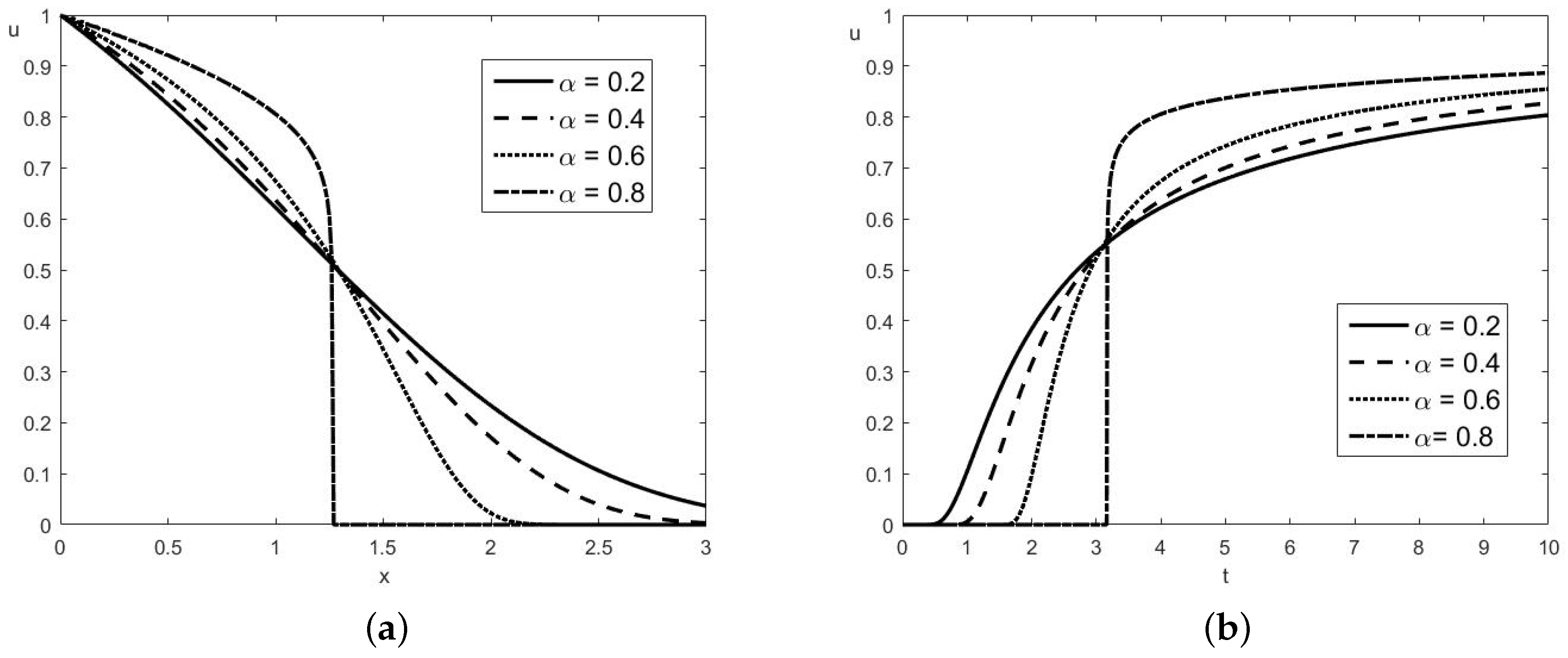
In Figure 1 the solution $u(x,t)$ is plotted for $\beta =0.8$ and four different values of $\alpha$: $0.2,0.4,0.6$, and $0.8$; $a={10}^{\alpha }$, $b={10}^{\beta -1}$. The case of instantaneous elasticity $\alpha =\beta =0.8$ is added to those plotted in Figure 1 of [17], in order to show the different behavior. In this case, the disturbance at $x=0$ propagates with finite speed $c=\sqrt{b/a}={10}^{-1/2}$ and $u(x,t)\equiv 0$ for $x>ct$. There is no wave front at $x=ct$. In the other three cases with $\alpha <\beta$ the propagation speed is infinite and $u(x,t)$ should be positive for all $x,t>0$. However, far from the wall, it becomes negligible. As expected, the solution $u(x,t)$ exhibits monotonic behavior: it is non-increasing with respect to x, see Figure 1a, and non-decreasing with respect to t, see Figure 1b. The plots presented in Figure 1a for $\alpha =0.2,0.4,0.6$ are identical with those given in Figure 1 of [17].

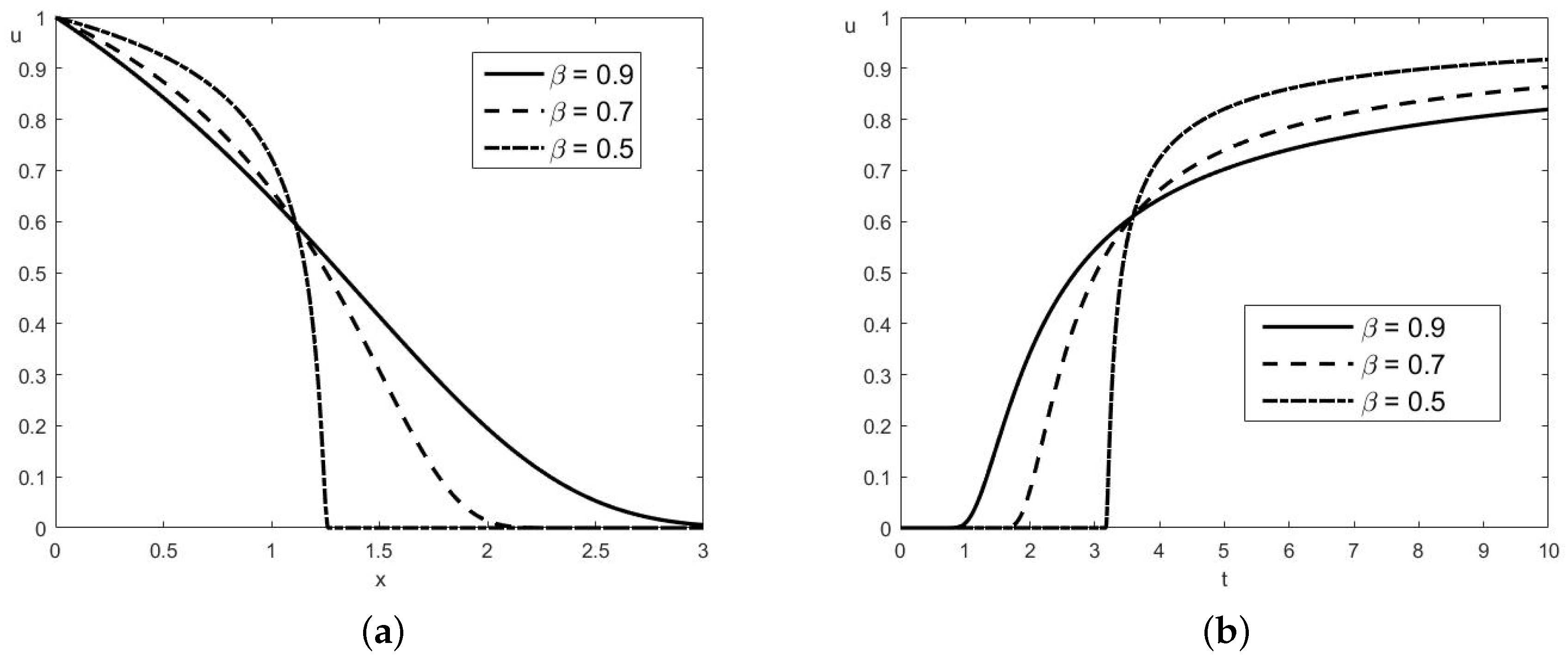
In Figure 2, the solution is plotted for $\alpha =0.5$ and three different values of $\beta$: $0.5,0.7,0.9$, $a={10}^{\alpha }$, $b={10}^{\beta -1}$. The case of instantaneous elasticity now is $\alpha =\beta =0.5$ with finite propagation speed c having the same value as above. Again, as expected, there is no wave front at $x=ct$. Monotonicity of $u(x,t)$ is clearly seen. The plots presented in Figure 2a for fixed time $t=4$ are identical with those given in [17], Figure 2.

We refer also to [33] (Figures 1–3) for more illustrations of the three different types of behavior, related to Maxwell fluids, namely: finite wave speed and presence of wave front ($\alpha =\beta =1$), finite wave speed and absence of wave front ($0<\alpha =\beta <1$), and infinite propagation speed ($0<\alpha <\beta \le 1$). Let us note that the paper [18] also presents plots of the solution of Stokes’ first problem for fractional Maxwell fluids with $\beta =1$. However, the plots in Figures 5a, 7a and 9a of [18] do not seem to be monotonically decreasing with respect to the spatial variable, which is a contradiction with the expected monotonic behavior of the solution.

5. Conclusions

The solution of Stokes’ first problem for a viscoelastic fluid with the generalized Maxwell model with fractional derivatives of stress and strain is studied based on its Laplace transform with respect to the temporal variable. The thermodynamic constraints on the fractional parameters imply physically reasonable monotonic behavior of solution with finite propagation speed (without wave front) when the two fractional orders coincide and infinite propagation speed otherwise. An explicit integral representation of the solution is derived and used for its numerical computation. The obtained numerical results are in agreement with those reported in [17].

The explicit integral representation of the solution can be further used to derive explicit or asymptotic expressions for other characteristics of the flow, such as shear stress at the plate, thickness of the boundary layer, etc.

The presented technique can be applied in the study of different generalizations of the considered model, e.g., the viscoelastic model based on Bessel functions in [34] and the fractional order weighted distributed parameter Maxwell model in [35].