
Effect of Directional Added Mass on Highway Bridge Response during Flood Events


1
Department of Civil and Environmental Engineering, The University of Iowa, Iowa City, IA 52242, USA
2
Iowa Technology Institute (ITI), The University of Iowa, Iowa City, IA 52242, USA
3
IIHR—Hydroscience and Engineering, The University of Iowa, Iowa City, IA 52242, USA
*
Author to whom correspondence should be addressed.
Infrastructures 2022, 7(3), 42; https://doi.org/10.3390/infrastructures7030042
Submission received: 9 January 2022
/
Revised: 1 March 2022
/
Accepted: 8 March 2022
/
Published: 16 March 2022
(This article belongs to the Special Issue Structural Performances of Bridges)
Abstract
:This article presents a new analysis to determine the variation in modal dynamic characteristics of bridge superstructures caused by hydrodynamic added mass (HAM) during progressive flooding. The natural frequency variations were numerically and experimentally extracted in various artificial flood stages that included dry conditions, semi-wet conditions, and fully wet conditions. Three-dimensional finite element modeling of both subscale and full-scale models were simulated through a coupled acoustic structural technique using Abaqus®. Experiments were performed exclusively on a subscale model at a flume laboratory to confirm the numerical simulations. Finally, an approach to quantify the directional HAM in the dominant axes of vibration was pursued using the concept of effective modal mass. It is shown that specific vibrating modes with the largest effective mass are strongly affected during artificial flood events and are identified as the dominant modes. Numerical simulation shows that large directional HAM is introduced on those dominant modes during flood events. For the full-scale representative bridge, the magnitude of the HAM along the first structural mode was estimated to be over 5.8 times the bridge’s structural modal effective mass. It is suggested that directional HAM should be included during the design of bridges over streamways that are prone to flooding in order to potentially be appended to the AASHTO code.
1. Introduction
Bridge structures are considered among the most vital infrastructure elements during and after severe weather incidents because their continued operation is necessary to facilitate the transportation of people, goods, and aid between communities. Based on US infrastructure reports, more than 40% of bridges have passed their designed lifespans, and about 10% are already structurally deficient. Among the human and natural contributors to highway bridge collapse under extreme conditions, hydraulic-related damage is a dominant factor in numerous collapse mechanisms [1,2]. It was reported that more than 48% of bridge collapses in the USA between 1989 and 2000 were due to hydraulic-related causes with various collapse mechanisms [3,4,5]. Destructive hurricanes such as Ivan and Katrina led to increased demand for investigation into these failure mechanisms; this requires sophisticated multi-physics modeling to capture the complex loading incidents on bridges during such extreme events. Recent experimental and numerical efforts have explored the forces imposed on bridge deck superstructures by hurricanes and flooding [6,7,8,9], but regulatory guidelines do not reflect the most recent findings. For example, AASHTO’s Guide Specifications for Bridges Vulnerable to Coastal Storms, which regulates instructions for estimating external forces and moments on bridge structures due to potential floods or storms [10], is based on the one-way fluid-structure interaction (FSI) theory. This means that external forces and moments are initially estimated with the assumption that the bridge is a rigid body, and the resulting forces are imposed upon a structural model. This approach neglects the mutual interactions between fluid forces and structural motions, which arise from fluid pressures and shear stresses introduced by structural motions. In particular, the fluid loading exerted in opposition to structural accelerations, termed hydrodynamic added mass (HAM), can cause tremendous changes in structural responses during flooding and storms. HAM is among the FSI considerations absent from the AASHTO code, which leaves inundated bridges vulnerable to excessive vibration amplitudes or unanticipated resonances.
Fluid-structure interaction theories vary widely in their formulations and simplifications. Most common formulations assume the timescale of structural vibration to be significantly smaller than the convective timescale of any surrounding fluid; such an approach also assumes structural vibrations to be relatively small in amplitude. Both assumptions are generally well suited to the structural responses of inundated bridges in moderate currents. Under such a model, the effective dynamics of the structure in question are altered by the kinematic and dynamic coupling of the fluid and structure. Additional hydrodynamic pressures acting on fluid–structure interfaces develop in proportion to structural accelerations, velocities, and displacements. The forces derived from these pressures are HAM, added damping, and added stiffness. These fluid forces consequently change the natural frequencies (NFs), modal participations, damping ratios, and, potentially, the mode shapes. Moreover, because these hydrodynamic forces are derived from local pressure distributions, their generalized/diagonalized forms depend strongly upon the mode shapes with which they are associated; low-order modes with large projected areas normal to their modal displacements tend to be most strongly affected.
The design and analysis of bridges and other critically important structures requires accurate assessment of the dynamic structural responses, which are strongly affected by the system modal characteristics that change so dramatically with the surrounding medium. Coupled acoustic structural (CAS) modeling is a mature FSI technique in which the fluid domain is approximated as acoustic elements that admit pressure and velocity modes within the fluid domain, while the structural domain is modeled using conventional structural elements. There are established theoretical formulations for computing added-mass quantities for simple geometries fully surrounded by unbounded fluid domains [11,12]. In practice, the added stiffness and damping are often neglected for relatively slow-moving fluids because their effect upon system dynamics is minimal, leaving only HAM to alter the system’s modal parameters [13,14]. For composite materials, complex geometries and mode shapes, and arbitrary inundation levels, estimates of HAM must be made numerically or experimentally. For example, the added mass effects on NFs of simple geometries such as annular, axisymmetric, and isotropic plates cannot be expressed explicitly; rather, their properties must be investigated numerically [15].
There are several commercial software packages with CAS modeling capabilities that can be used to simulate FSI coupling and extract eigenfrequencies and eigenmodes for a diverse set of FSI scenarios. Applications range from a laminated composite plate vibrating in wet conditions to earthquake-induced sloshing of liquid tanks [16,17]. For containership structures, numerical studies show an up to 30% change in NFs as the composition of the surrounding fluid varies [18]. The effects of varied immersion of composite plates in a dense fluid, along with the effects of material anisotropy on HAM, were explored by Motley et al. [19] and Kramer et al. [20], who demonstrated a reduction of nearly 50% in NFs for steel plates and an 80% reduction for composite plates as those plates were immersed in water. Free vibration of partially submerged surface-piercing struts in multi-phase flow demonstrated both experimentally and numerically that HAM effects could change the ordering of normal modes [21]. Time history analysis of a liquid storage tank to study sloshing effects was performed under several bi-directional earthquakes using CAS and finite element method (FEM) tools [22]. Bend-twist coupled behavior of a composite hydrofoil and the effect of its fiber angle were numerically investigated under dry and wet conditions by CAS simulation [23].
The effect of HAM of hydrofoil and its trailing edge shape effect was numerically studied thoroughly [24], and a numerical CAS technique was successfully applied to simulate the FSI of a clamped hemispherical shell structure with good agreement with experimental results [25]. Experimental and numerical modal dynamic sensitivity analysis indicated that the NFs of bridge piers could change up to 20% while the river stream level rises [26]. It was proven that, for small-scale, flexible, soft structures, the experimental modal characteristics are consistent with the numerical results in a wide frequency range [13]. However, for larger structural models such as hydrofoils, FSI studies are frequently numerical rather than experimental [24]. Experimental data for slender hydrofoil structures exist for very few initial vibrating modes, with up to 7.64% error between the experimental and numerical modal information [27]. Estimates of modal HAM, added stiffness, and added damping for a hydrofoil were experimentally estimated by Harwood et al. [28], but only as percentages of the associated structural modal properties. Base shear force, base moment, and HAM properties for immersed columns with arbitrary cross-section have been numerically calculated [29].
While CAS simulation is a useful tool for prediction of coupled FSI, it comes at the cost of increased computational expense, more complex simulation setup, and limitations on its applicability, such as low flow speeds. Another simpler method for modeling the effects of HAM is accomplished by substituting the fluid domain with structural mass elements to produce the same mass-loading distribution that would result from a fluid-filled domain. Equivalent systems for sloshing fluid in arbitrary-section aqueducts during artificially seismic events were studied, and the structural time history responses were computed during simulated events [30]. A lumped mass stick model for nuclear containment buildings based on modal characteristic properties was proposed and numerically compared to the original FEM that showed promising results [31]. It is a common approach to substitute the fluid domain of a reservoir tank with discrete lumped mass elements numerically to investigate effects under vibration and stress/strain field calculations. Each mass element is derived at each tank elevation from the pressure distributions at each assumed vibrating mode. The equivalent system for a water-surrounded hollow bridge pile was derived by evenly distributing discrete mass elements along the pile’s height [32]. Numerical simulation indicated an up to 23% change in NFs as the water height varied around the pile due to the HAM. An equivalent structural system to be substituted with a CAS problem was investigated for a piping system application with both numerical and experimental setups [33].
The use of equivalent uniformly distributed mass to perform simplified FSI analysis is challenged by two principal issues. The first is that fluid inertial loading is not necessarily uniform, especially for complex flows involving multiple phases and free surfaces. The second issue is that fluid inertial loading is directional, so treating HAM as isotropic is generally inaccurate. The AASHTO design code does not explicitly consider the change of medium, so there is a need for simple and efficacious predictive methodologies that can approximate HAM effects without the need for specialized simulation. The objective of this work is to emphasize the importance of—and the need to consider—non-uniform HAM for bridges at risk of flooding. To accentuate the effects of medium changes during inundation flood stages, this work presents both numerical and experimental studies performed on a small-scale model as a validation step, followed by numerical simulation on a full-scale model. The progression of flood events was defined as dry condition, semi-inundation, and full inundation. A CAS solver was used to estimate variation of NFs during simulated flood events; then a process was proposed to quantify modal HAM with the same quantity unit as the original unit of the structural mass from the effective modal mass magnitude. The proposed approach can compute directional HAM by using effective modal mass factors that non-uniformly affect bridges during varying flood conditions.
2. Materials and Methods
Governing Equations of Coupled Acoustic Structure (CAS)
2.1. Acoustic Domain Theory
The governing partial differential equation for the acoustic fluid domain is the well-known Helmholtz wave equation, expressed as follows [34]:
where is the acoustic pressure and is the speed of sound in the surrounding acoustic domain, which can be expressed as follows:
where and are the bulk modulus and mass density of the fluid medium, respectively. By assuming irrotationality of the flow, the velocity field is taken to be a conservative vector field, expressed as the gradient of a potential function, :
where is the gradient operator; , , and are the velocity terms along the x, y, and z axes, respectively; and is the fluid displacement vector. The fluid acoustic pressure is related to the scalar velocity potential by the unsteady Bernoulli equation,
If the fluid medium is further assumed to be incompressible (e.g., water), Equation (1) is replaced by the Laplace equation to ensure continuity:
In this case, the distribution of pressure inside the acoustic domain is governed by the elliptic boundary value problem on the scalar potential . For analytical coupling, it can be advantageous to construct a modal model of the fluid and structure, where kinematic and dynamic boundary conditions specified on the interface between the structural and acoustic domains are used to find modal potentials under the simplifying assumption of infinite acoustic speed. However, most numerical solvers (e.g., FEMs or boundary element methods) retain Equation (1) for the sake of generality, using large values for the bulk modulus to correctly approximate the acoustic speed in the fluid domain.
2.2. Coupling Solid and Acoustic Domains
CAS is multi-physics coupling analysis that contains both solid and fluid domain formulations to be simultaneously solved. The discrete FEM formulation of the CAS model can be expressed by the following asymmetric matrix formulations in homogeneous form [22,25]:
In the case of free vibration, Equation (5) is rewritten as follows:
where , , , , , and are the displacement degree of freedom (DOF) vector, the fluid acoustic pressure DOF, the mass, damping, and stiffness matrices, and the reaction impedance, respectively. In all cases, the subscript indicates a structural quantity and the subscript indicates a fluid quantity. The displacement vector includes both structural and fluid displacements. The coupling between the two mediums is enforced by maintaining equal normal displacement/velocity (kinematic coupling) and equal normal stresses (dynamic coupling) at the interface between the solid and fluid domains. Matrix is critical to the coupling of the fluid and structure by enforcing the compatibility of pressure and displacement at the interface. Under an assumption of proportional damping, Equations (6) and (7) may be diagonalized and a modal model may be realized by an appropriate eigenproblem solver. In total, the solver returns the homogenous solution of Equations (6) and (7) for N modes in terms of the nth NF () and the nth eigenvector containing both structural and fluid acoustic pressure modes . Through manipulation of the aforementioned coupling formulas, it can be shown that added mass and added damping elements of the mass and damping matrix can be expressed as follows [35]:
where , , , and are the real and imaginary operator, normal unit vector, and whole wet surface at the fluid and structure interfaces, respectively. Equations (8) and (9) represent projections of the pressure fields associated with mode onto structural mode . It is clear that neither HAM nor added damping elements can be expressed as spatial mass or damping matrices because they are functions of frequency, structural mode shapes, and velocity potential field—which is itself a solution to a boundary value problem [36,37]. It has been indicated that flood-prone bridges experience significant excitations in the lower frequency range during flooding events, and also that the dynamic characteristics (NFs, damping, and mode shapes) for lower modes vary much more than those of higher-frequency modes [38,39]. Due to these facts and knowing that bridge structural systems are stiff enough that only the first few initial modes are operationally excited, the practical HAM consideration should be attributed to the initial structural modes.
2.3. Essential Boundary Conditions
There are three common types of boundary conditions (BCs) for CAS problems that must be satisfied on the fluid-structure and fluid-free-surface interfaces [40]. Because all three are used in the present simulations, they will be briefly described in this section.
2.3.1. Imposed Pressure (Dirichlet BCs)
On the free surface of the fluid domain, the pressure must be enforced to be equal to zero. The first-order hydrodynamic pressure at any point of the fluid domain is simplified from the unsteady Bernoulli equation:
On the free surface (), a constant pressure condition is imposed as
2.3.2. Imposed Kinematics (Neumann BCs)
Within the acoustic domain, the assumption of inviscid (shear-free) flow, coupled with a small-displacement assumption, allows the first-order perturbations on fluid pressure and acceleration to be related anywhere in the fluid domain (), as follows:
At the fluid–solid interface, the kinematic coupling dictates that fluid and solid velocities and accelerations must be equal:
where and are the structural acceleration and the outward normal direction of the interface surface at fluid domain, respectively. This type of BC is applied on the interface of the fluid and the solid as the geometric compatibility condition.
Where the fluid domain is bounded by stationary wall (e.g., the rigid bottom and side walls of a flume), the velocity and acceleration are identically zero; consequently, Equation (13) will reduce to a zero-gradient condition at those boundaries:
2.3.3. Imposed Impedance or Admittance (Robin BCs)
Where the acoustic domain is not physically bounded, two kinds of BCs may be imposed in order to simulate far-field energy dissipation. These are typically either absorbing BCs or infinite element implementations, both of which require definitions of the impedance and admittance. The level of wave energy absorption at far-field BCs can be defined in terms of acoustic impedance (Z) or its reciprocal, admittance (A):
At the far-field boundaries of an FSI simulation, a Robin-type BC is used to model nonreflecting waves or absorbing BCs to minimize reflected energy effects. The detailed implementation is available in the literature [41]. This BC plays an important role on structural responses, and therefore, its characteristic must be prudently prescribed. Impedance and admittance BCs are based on structural size, scaling, material types, and several other considerations to better predict real-world interaction behavior, even for large structures like a dam reservoir [42].
3. Numerical and Experimental Implementation
As indicated in Section 2.2, there is no explicit formula or analytical derivation to calculate added mass for complex systems such as highway bridge structures. Therefore, the effect of fluid inertial loading can only be investigated through numerical and experimental approaches. In this section, a prototype bridge and its small-scale physical model are first described. Next, the numerical modeling at both scales is introduced. Finally, the experimental approach and data acquisition system used to test the small-scale model in various flood steps are described.
3.1. Prototype Bridge Models
The prototype bridge was selected by picking up one span of a representative composite-deck, steel-girder bridge system, which is the prevalent type in the USA. This representative bridge model is located near Cedar Rapids, Iowa and carries US highway 30 over the Cedar River as shown in Figure 1a. It has a federal ID of FHWA #33472, a span length of 45.7 m, and was investigated in another study as well [43]. This specific bridge has experienced complete inundation by flood incidents during recent years, as indicated by reports at the Iowa DOT.
3.2. Small-Scale Physical Model
The small-scale model of the FHWA #33472 representative bridge was constructed at a geometric scale factor of 1:60 while observing similarity to the degree possible and practical. A single span was constructed from an aluminum plate with girders and pinned connections at each end. Additional masses were included along the edges of the model to approximate the mass distribution of the protype span, shown in Figure 1b. The model was tested in a narrow flume with a controlled water depth, described further in Section 3.4. The construction of a small-scale model with regards to material type, added concentrated physical masses, and structural stiffness necessary to ensure similarity is provided by Karimpour et al. [5,43]. In-depth conceptual information regarding small-scale structural modeling based on prototype size, type, materials, and aims of prospective experiments is also available in the literature [14,44].
3.3. Numerical CAS Implementation
CAS simulation is one of several robust, commercially available multi-physics tools that enable accurate simulation, prediction, and analysis of sophisticated engineering problems [45]. Simulation of CAS can be accomplished by bounding the structural elements with acoustic elements to comply with both solid and fluid governing equations and coupling conditions. The commercial software Abaqus® was used to numerically estimate the mode shapes and NFs of the systems under both dry and wet conditions [46]. The 3D liquid domain was modeled by the eight-node acoustic element type of AC3D8 with an hourglass control option. For the small-scale bridge model, four-node shell elements with reduced integration points (S4R) and hourglass control were used to model the bridge deck and girders. Inertia elements of type MASS were used to model concentrated added masses, which were attached to the small-scale physical model. The final small-scale FEM contained 10,568 structural nodes and 143,094 acoustic nodes.
In Figure 2, the FE model of the small-scale bridge plus three dominant mode shapes (defined as those with maximum modal participation factors) are shown in dry conditions. Based on the FEM results, the 1st, 4th, and 17th modes are dominant and contribute the most to vibration of the small-scale model along its vertical axis (gravitational direction). Figure 3 and Figure 4 show the FEM-CAS modeling of the small-scale model during the semi-inundation and full-inundation stages, respectively. Increasing inundation conditions were simulated by raising the height of the acoustic fluid domain until the upper acoustic boundary was coincident with the deck level (semi-inundated) and completely covered the deck by a height equal to the bridge girder depth (fully inundated). Air has a negligible mass loading effect, so the dry portions of the models were treated as in vacuo. It can be observed that, for conditions of both semi-inundation and full inundation, those aforementioned modes (1st, 4th, and 17th) remain the modes with the highest modal participation factors. This signifies that a change in the fluid medium does not significantly alter the mode shapes or their relative participation but that it does change the NFs of the system.
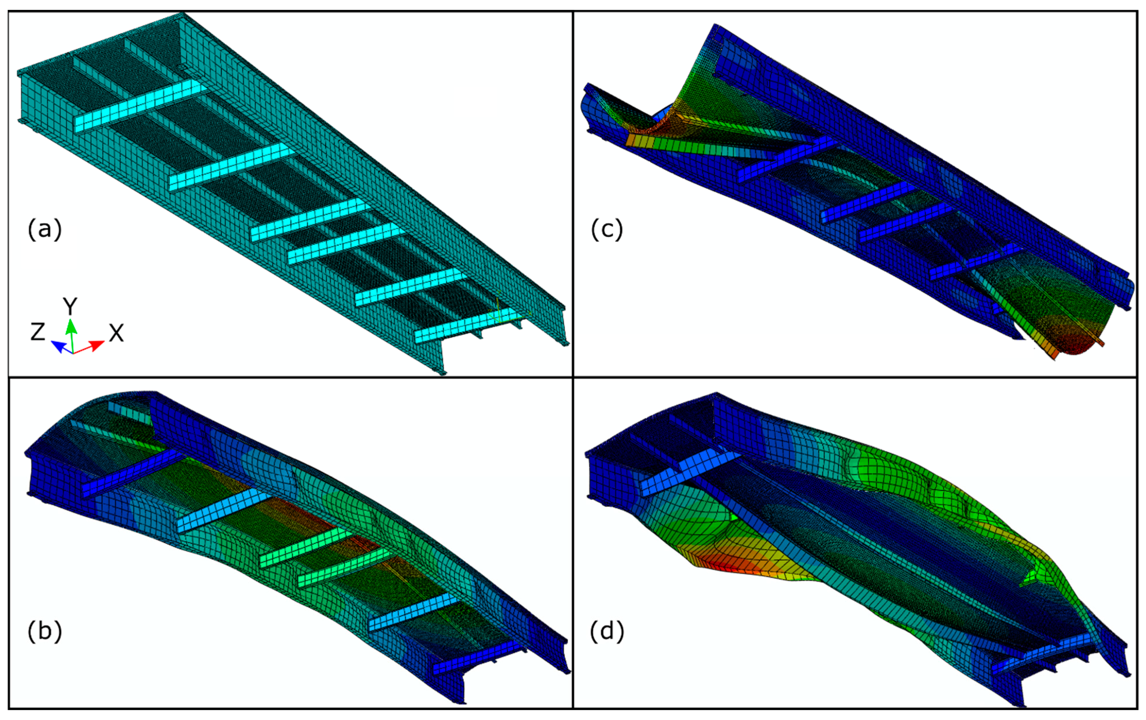
For the full-scale bridge FE model, 3D shell elements (type S4R) were used to model girders and cross beams, 3D truss elements (type T3D2) were used to simulate rebar and stirrups embedded in the concrete deck, and 3D brick elements with reduced integration points (C3D8R) were assigned to the concrete slab. The full-scale bridge FE model is made up of 645,720 structural nodes and 284,962 acoustic nodes. Figure 5 shows the FEM-CAS mesh describing the full-scale bridge, along with three dominant mode shapes. Figure 6 and Figure 7 show the semi-inundation and full-inundation stages of the same full-scale model. The dominant extracted modes for the full-scale bridge are the 1st, 4th, and 9th modes, whereas the 1st, 4th, and 17th modes were dominant for the small-scale bridge. Perfect similarity across widely disparate geometric scales is nearly impossible to maintain; in general, the priority is to match the lower-order modes rather than the higher-order ones because the lower-order modes tend to participate more than higher-order modes during structural vibration. In this particular case, the simplified geometry was suitable to reproduce the balance of modal participation through at least the 4th mode, but not beyond the 9th mode.
For both the small-scale and full-scale FE models, the fluid–solid coupling was enforced through kinematic BCs (displacement equality at the interface) as well as dynamic BCs (pressure equality at the interface). The FE mesh size was refined through convergence analysis in two steps. First, the solid mesh size in dry conditions was refined until the first 10 NFs of the solid model varied by less than 1%. In the second step, the coupled fluid–solid model in wet conditions was refined until the coupled NFs also varied by less than 1% for the 10 initial modes. The numerical eigenfrequency extraction was done based on the Abaqus Lanczos eigenvalue solver method in both dry and wet simulated conditions. Linear perturbation and small displacement assumptions were considered. Several assumptions were considered during CAS and FEM modeling in this study. The fluid domain assumptions can be enumerated as follows: irrotational, inviscid, no material flow, no mesh distortion, and linearly compressible fluid—albeit with a high bulk modulus. Additionally, a nonslip condition exists at rigid (unmoving) walls. Material damping and gravitational loading were both neglected in the structure. The properties of materials modeled in the FEM-CAS simulations are listed in Table 1.
3.4. Experimental CAS and Data Collections
To demonstrate the validity of the numerical simulation, a physical experiment was executed using a small-scale model with the objective of quantifying NFs at varying degrees of inundation in a model-scale flume. To obtain a high signal-to-noise ratio across a broad frequency spectrum and obtain reliable mode estimates in the flume environment, measurements were made of both accelerations and bending strains. A single waterproof accelerometer was recorded for three roving hammer tests. In a separate trial, six strain gauges were recorded for two roving hammer tests, with the strain measurements utilized for feature extraction. A DEWESoft® data acquisition system (DEWE-43A model) was used to acquire data at a sampling rate of 1000 Hz at 24-bit resolution. A low-pass filter with cutoff frequency of 220 Hz was implemented on all channels. As shown in Figure 8, the small-scale bridge model installed in a flume in three predefined stages similar to those of the FEM-CAS simulation are shown in dry conditions (Dry), semi-inundation (WET-0), and full inundation (WET-1).
3.5. Experimental Modal Parameter Extraction
Output-only system identification was performed, using the frequency domain decomposition (FDD) approach, to extract NFs and damping for individual modes. The FDD approach is deployed as an output-only method [47,48,49] that expresses the response power spectrum densities (PSDs) matrix that attains the same poles as the frequency response function (FRF). The singular value decomposition (SVD) of the response PSDs matrix is used to extract the system NFs and mode shape components, as follows [43,50]:
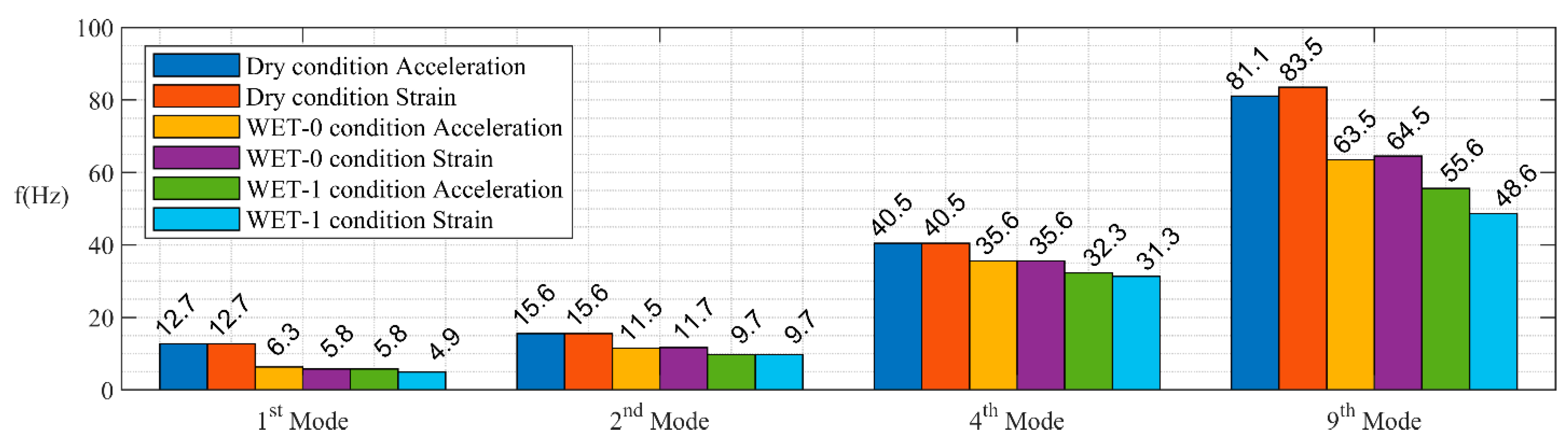
where , , and are unitary matrices containing unscaled mode shape components, the Hermitian transpose of , and a diagonal matrix containing the scalar values of the system poles. Figure 9 and Figure 10 show the acceleration and strain time domain and frequency domain results, respectively. Time-domain traces are shown in the first column of each figure, the PSD in the second column, and the SVD in the third column, with detected system poles indicated by vertical dashed lines. Figure 11 summarizes the detected NFs for each stage of inundation using strain and acceleration signals. As shown in Figure 11, there are slight differences between the natural frequencies extracted from the strain signals and those from the acceleration signals. Those differences, while minor, do suggest a difference in the quality of the respective signals. In this work, the frequencies identified from measured accelerations were used because accelerometers tend to have higher sensitivities, better noise immunity, and better signal-to-noise ratios than strain gauges at relatively high frequencies.
It is immediately clear that the NFs decrease with progressive stages of inundation—a product of the HAM. There is some discrepancy between the accelerometry and strain measurements that grows with increasing modal frequency; this is attributed to the reduced signal-to-noise ratio in the strain measurements at higher frequencies, which is thought to degrade the system identification slightly.
4. Quantification of HAM by Modal Effective Mass
As explained earlier, the HAM of a mode is typically not a unique value because it varies with the scaling convention used for the mode shapes. This section aims to quantify unique modal HAM values in a unique and physically intuitive manner by leveraging the concept of modal effective mass. The nth fundamental frequency of the dry structural system can be expressed in terms of nth modal stiffness and nth modal mass as follows:
Under the assumption of a nearly quiescent fluid, the fluid-added stiffness is conventionally neglected, leaving only the HAM effect when the structure is immersed. The omission of the fluid-added stiffness is not strictly valid when the structure is located at the fluid-free surface; the changing displacement will produce a buoyant force that manifests as a weak spring. However, the fluid-added stiffness should be of minimal importance for relatively dense structural materials such as bridges, and in the scope of this research, its effect was considered negligible. Therefore, the system’s nth NF can be estimated by the following formula [13]:
where is the HAM. The reduction in NFs of the nth mode as a percentage of the dry value is denoted by and expressed as follows:
The HAM coefficient, which is the ratio of HAM to the dry modal mass of the nth mode, can be expressed using Equations (18) and (19) as follows:
Equation (21) indicates that a unique quantification of HAM requires NFs in dry and wet conditions and a uniquely valued dry modal mass. Modal mass, however, is not explicitly reported by FEM solvers; rather, they return modal participation factors and effective modal mass. For the th mode of a structural system, the th modal participation factor in the ith direction indicates how much motion in the th global direction (X-Y-Z) is contributed by the th eigenvector, calculated as follows:
where is the th column vector of the rigid-body “influence” matrix describing the displacement of masses resulting from a rigid-body displacement along the ith axis. The nth modal mass is calculated by diagonalizing the spatial mass matrix with the th eigenvector estimated by the FEM solver:
As previously noted, the generalized modal mass is a non-unique value with no physical meaning because the eigenvector scaling is arbitrary depending on the method used to approximate the eigensolution. The modal participation factor in Equation (22) can be further exploited to cancel out the arbitrary scale factor to arrive at the uniquely defined parameter known as effective modal mass, which possesses the same units as the physical system mass. The nth effective modal mass of the system along the ith direction can be estimated as follows [41]:
Unlike the generalized modal mass () that introduces uniform lump mass in the modal domain, the effective modal mass possesses physical interpretation in the spatial domain along all 3D coordinate directions (i). Each term of the effective modal mass can be interpreted as if an acceleration in the ith global direction (X-Y-Z) is imposed on the structure, and a percentage of the imposed inertial force equal to is attributed to the nth mode of the system. Thus, the modes with the highest effective modal masses contribute the most to the structural dynamic response if the input spectrum has a relatively uniform distribution in the frequency domain. Furthermore, the summation of effective masses in a single direction (i) for all system modes is equal to the system’s total mass, as follows:
where and are the total weight of the structure and the gravitational constant, respectively. Typically, just a few modes represent a very high percentage of the effective mass; these modes are dubbed the dominant mode hereafter. In this study, a dominant mode is defined as any mode for which the effective modal mass in any direction is more than 1% of the dry structural mass. The physical interpretation and uniqueness of the effective mass quantity makes it an excellent candidate for realizing physical HAM values. If the effective modal mass values have been identified from FEM-CAS solver output, they may be substituted into Equation (21) in lieu of the generalized modal mass to derive and estimate the directional HAM as follows:
Table 2 presents the results of numerical and experimental features for the small-scale model for dominant modes—determined to be the 1st, 4th, and 17th modes. The NF column reports FEM results with experimental measurements included in parentheses when available. The overall mass of the physical small-scale bridge model is 5.05 kg. While effective modal mass is directional, the analysis here was limited to the vertical direction because an overwhelming majority of the fluid dynamic pressures act on surfaces with a vertical surface normal, and a majority of the dominant mode shapes represent vertical displacement of the bridge surface. The percentage reduction in NFs is reported for both semi-inundation and full inundation.
Finally, HAM values were calculated through Equation (26), and their percentage relative to the structure’s total mass is reported in parentheses. In contrast to the generalized modal mass and common uniform HAM concept, Equation (26) is deployed to compute the practical/feasible directional HAM along the most critical coordinate direction of the system’s vibration. In the case of bridge structures, this most critical direction is vertical, in the direction of gravity. This is a significant distinction because it means that HAM does not act equally in all coordinate directions. Rather, the HAM in one direction can be very large while it is negligibly small in other directions. Table 2 indicates that, for the small-scale model, 81% of the effective modal mass in the vertical direction is contained in the first structural mode alone. Moreover, the semi-inundation and full-inundation stages produce HAM equal to 280% and 403% of the overall dry mass of the model, respectively. Results of simulations of the full-scale representative bridge span are reported in Table 3.
For the full-scale model, the 1st, 4th, and 9th modes were retained as dominant modes. It was found that the overall mass of one span bridge is about 570 metric tons. Numerical simulation shows that up to 3.75 and 5.85 times the mass of the bridge itself would be introduced as directional HAM in the semi-inundation and full-inundation phases, respectively. This huge fluid inertial load along the vertical direction is associated with very low NFs, where excitation is most likely to occur during flood and storm events, suggesting a dramatic increase in the risk of excessive stress/strain in primary structural components during flooding.
5. Discussion and Results
The current AASHTO guidelines available for bridges subjected to flooding consider bridges as rigid structures and use formulas to estimate the resulting fluid forces that can be applied to the bridge. These AASHTO formulas do not include the variation in bridge response as a result of FSI, leaving the risk of FSI resonance and excessive inertial loads unevaluated. This article demonstrates the importance of considering the HAM effects on bridges that are vulnerable to floods. In order to compute non-uniform directional HAM, the effective modal mass quantity was employed as a physically meaningful quantity to scale the added mass coefficient. The effective modal mass was found to be suitable because it indicates how much inertial force the nth mode along the ith coordinate direction contributes to the system’s overall physical mass. Furthermore, it has the same physical unit as the structural mass, making the calculation more sensible for comparison.
Because its summation along individual axes for all vibrating modes must be equal to the gross mass of the system, it becomes convenient to use it to evaluate the relative contributions of dynamic modes under excitation incidents. This study found that a few dominant modes of vibration of the bridge structure accounted for a very high percentage of the total effective modal mass, meaning that they are the most inertially active responses to excitation. About 81% and 72% of the effective modal mass are attributed to just the first mode of bridge structures with hinge connections for small-scale and full-scale bridges, respectively. Both small-scale and full-scale models of the representative bridge show the same dominant modes at the 1st, 4th, and 17th modes, suggesting that similarity was well-maintained across geometric scales, allowing us to replicate real-world scenarios in small-scale modeling.
In the proposed approach, Equation (26) was derived to compute directional HAM from the dry and wet NFs as well as effective modal mass under dry conditions. FEM-CAS solvers are able to compute both NFs and modal effective mass for composite structures such as bridges. For a small-scale bridge during the semi-inundation stage, HAM values along the vertical axis are 280%, 2.3%, and 5.7% of the bridge’s dry mass for the 1st, 4th, and 17th modes, respectively. During the full-inundation stage, those values are 403%, 4.1%, and 10% of the dry mass for the same modes. At full scale, which was only evaluated using simulation, semi-inundation produced HAM values along the vertical axis of 375%, 34%, and 16% of the dry mass of the bridge for the 1st, 4th, and 17th modes, respectively. During full inundation, those values are 585%, 50%, and 35% of the dry mass. Neither these dynamic property variations (NF variations) nor the huge amount of non-uniform HAM are directly considered in the AASHTO code. This omission leads to safety concerns for bridges that are partially or fully inundated, where external excitation may promote unanticipated resonances with much greater mass participation than in dry conditions.
While this work suggests a method for assigning a unique value to the HAM, the re-spatialization of that mass so that it may be approximated using a distribution of point masses in the dry model remains an area for future work. With detailed knowledge of the mode shapes, it is possible to approximate the HAM mass matrix through the inverse of the modal diagonalization process, but errors in the mode shape—or changes in the mode shape with changing immersion—mean that this method will produce only an approximation of the spatial HAM matrix. Future work should evaluate the effects of mode shape estimates upon the resulting mass matrix. Additionally, this methodology will be inherently limited to cases in which the dry and wetted mode shapes are substantially the same, so an extension of this work should evaluate the consistency of mode shapes using the Modal Assurance Criterion (MAC) or similar metrics.
In this study, it was shown that, for heavy bridge structures, the main axis that could be excited during a potential storm is the axis along the gravitational (heave) direction; additionally, all bridge boundary conditions were considered as rocker bearings that behave like hinges without lateral movement. Real bridges mostly sit on partially restricted supports, such as pendulum, elastomeric, lead-rubber bearings, etc., rather than fixed ones, at least at one of their span ends. Thus, they can expand freely in response to external environmental or operational effects without producing internal stress. It is strongly suggested that further studies be executed to consider a bridge system with roller bearings and continuous span systems that could be displaced laterally by incoming floods, which most likely causes unseating incidents.
Further numerical studies are required to derive a simplified formula based on regression analysis that a bridge designer could use in addition to the proposed formula for estimation of HAM of such bridges. The results of the proposed numerical approach could help bridge designers better consider the dynamic/inertial force that is missing in the AASHTO code for bridges over conduits and streamways.
Author Contributions
A.K.: Conceptualization, Data curation, Formal analysis, Investigation, Methodology, Software, Validation, Writing—original draft. C.H.: Conceptualization, Data curation, Formal analysis, Investigation, Methodology, Writing—review and editing. S.R.: Conceptualization, Data curation, Formal analysis, Investigation, Methodology, Project administration, Resources, Writing—review and editing. All authors have read and agreed to the published version of the manuscript.
Funding
The research described in this paper is funded by the Mid-America Transportation Center via a grant from the U.S. Department of Transportation’s University Transportation Centers Program (grant number: DOT 69A3551747107), and this support is gratefully acknowledged. The contents reflect the views of the authors, who are responsible for the facts and the accuracy of the information presented herein and are not necessarily representative of the sponsoring agencies.
Institutional Review Board Statement
Not applicable.
Informed Consent Statement
Not applicable.
Conflicts of Interest
The authors declare no conflict of interest.
References
- Deng, L.; Wang, W.; Yu, Y. State-of-the-art review on the causes and mechanisms of bridge collapse. J. Perform. Constr. Facil. 2016, 30, 04015005. [Google Scholar] [CrossRef]
- Prendergast, L.J.; Limongelli, M.P.; Ademovic, N.; Anžlin, A.; Gavin, K.; Zanini, M. Structural health monitoring for performance assessment of bridges under flooding and seismic actions. Struct. Eng. Int. 2018, 28, 296–307. [Google Scholar] [CrossRef] [Green Version]
- Wardhana, K.; Hadipriono, F.C. Analysis of recent bridge failures in the United States. J. Perform. Constr. Facil. 2003, 17, 144–150. [Google Scholar] [CrossRef] [Green Version]
- Robertson, I.N.; Riggs, H.R.; Yim, S.C.; Young, Y.L. Lessons from Hurricane Katrina storm surge on bridges and buildings. J. Waterw. Port Coast. Ocean Eng. 2007, 133, 463–483. [Google Scholar] [CrossRef]
- Karimpour, A.; Rahmatalla, S.; Markfort, C. Identification of damage parameters during flood events applicable to multi-span bridges. J. Civ. Struct. Health Monit. 2020, 10, 973–985. [Google Scholar] [CrossRef]
- Qu, K.; Sun, W.Y.; Kraatz, S.; Deng, B.; Jiang, C.B. Effects of floating breakwater on hydrodynamic load of low-lying bridge deck under impact of cnoidal wave. Ocean Eng. 2020, 203, 107217. [Google Scholar] [CrossRef]
- Xiang, T.; Istrati, D.; Yim, S.C.; Buckle, I.G.; Lomonaco, P. Tsunami loads on a representative coastal bridge deck: Experimental study and validation of design equations. J. Waterw. Port Coast. Ocean Eng. 2020, 146, 04020022. [Google Scholar] [CrossRef]
- Yang, W.; Lai, W.; Zhu, Q.; Zhang, C.; Li, F. Study on generation mechanism of vertical force peak values on T-girder attacked by tsunami bore. Ocean Eng. 2020, 196, 106782. [Google Scholar] [CrossRef]
- Santo, H.; Taylor, P.H.; Dai, S.S.; Day, A.H.; Chan, E.S. Wave-in-deck experiments with focused waves into a solid deck. J. Fluids Struct. 2020, 98, 103139. [Google Scholar] [CrossRef]
- Kulicki, J.M.; Mertz, D.R. Guide Specifications for Bridges Vulnerable to Coastal Storms; AASHTO: Washington, DC, USA, 2008. [Google Scholar]
- Patel, M.H. Dynamics of Offshore Structures; Butterworth-Heinemann: Oxford, UK, 2013. [Google Scholar]
- Newman, J.N. Marine Hydrodynamics; The MIT Press: Cambridge, MA, USA, 2018; p. 448. [Google Scholar]
- Escaler, X.; De La Torre, O.; Goggins, J. Experimental and numerical analysis of directional added mass effects in partially liquid-filled horizontal pipes. J. Fluids Struct. 2017, 69, 252–264. [Google Scholar] [CrossRef]
- Deng, Y.; Guo, Q.; Shah, Y.I.; Xu, L. Study on modal dynamic response and hydrodynamic added mass of water-surrounded hollow bridge pier with pile foundation. Adv. Civ. Eng. 2019, 2019, 1562753. [Google Scholar] [CrossRef] [Green Version]
- Askari, E.; Jeong, K.H.; Ahn, K.H.; Amabili, M. A mathematical approach to study fluid-coupled vibration of eccentric annular plates. J. Fluids Struct. 2020, 98, 103129. [Google Scholar] [CrossRef]
- Sharma, N.; Mahapatra, T.R.; Panda, S.K.; Mazumdar, A. Acoustic radiation characteristics of un-baffled laminated composite conical shell panels. Mater. Today Proc. 2018, 5, 24387–24396. [Google Scholar] [CrossRef]
- Rawat, A.; Mittal, V.; Chakraborty, T.; Matsagar, V. Earthquake induced sloshing and hydrodynamic pressures in rigid liquid storage tanks analyzed by coupled acoustic-structural and Euler-Lagrange methods. Thin-Walled Struct. 2019, 134, 333–346. [Google Scholar] [CrossRef]
- Sepehrirahnama, S.; Xu, D.; Ong, E.T.; Lee, H.P.; Lim, K.M. Fluid–structure interaction effects on free vibration of containerships. J. Offshore Mech. Arct. Eng. 2019, 141, 061603. [Google Scholar] [CrossRef]
- Motley, M.R.; Kramer, M.R.; Young, Y.L. Free surface and solid boundary effects on the free vibration of cantilevered composite plates. Compos. Struct. 2013, 96, 365–375. [Google Scholar] [CrossRef]
- Kramer, M.R.; Liu, Z.; Young, Y.L. Free vibration of cantilevered composite plates in air and in water. Compos. Struct. 2013, 95, 254–263. [Google Scholar] [CrossRef]
- Harwood, C.; Stankovich, A.; Young, Y.L.; Ceccio, S. Combined experimental and numerical study of the free vibration of surface-piercing struts. In Proceedings of the 16th International Symposium on Transport Phenomena and Dynamics of Rotating Machinery, Honolulu, HI, USA, 10–15 April 2016. [Google Scholar]
- Rawat, A.; Matsagar, V.A.; Nagpal, A.K. Numerical study of base-isolated cylindrical liquid storage tanks using coupled acoustic-structural approach. Soil Dyn. Earthq. Eng. 2019, 119, 196–219. [Google Scholar] [CrossRef]
- Liao, Y.; Garg, N.; Martins, J.R.; Young, Y.L. Viscous fluid–structure interaction response of composite hydrofoils. Compos. Struct. 2019, 212, 571–585. [Google Scholar] [CrossRef]
- Zeng, Y.S.; Yao, Z.F.; Zhou, P.J.; Wang, F.J.; Hong, Y.P. Numerical investigation into the effect of the trailing edge shape on added mass and hydrodynamic damping for a hydrofoil. J. Fluids Struct. 2019, 88, 167–184. [Google Scholar] [CrossRef]
- Eslaminejad, A.; Ziejewski, M.; Karami, G. An experimental–numerical modal analysis for the study of shell-fluid interactions in a clamped hemispherical shell. Appl. Acoust. 2019, 152, 110–117. [Google Scholar] [CrossRef]
- Deng, Y.; Guo, Q.; Xu, L. Experimental and numerical study on modal dynamic response of water-surrounded slender bridge pier with pile foundation. Shock Vib. 2017, 2017, 4769637. [Google Scholar] [CrossRef]
- Liu, X.; Zhou, L.; Escaler, X.; Wang, Z.; Luo, Y.; De La Torre, O. Numerical simulation of added mass effects on a hydrofoil in cavitating flow using acoustic fluid–structure interaction. J. Fluids Eng. 2017, 139, 041301. [Google Scholar] [CrossRef]
- Harwood, C.M.; Felli, M.; Falchi, M.; Garg, N.; Ceccio, S.L.; Young, Y.L. The hydroelastic response of a surface-piercing hydrofoil in multiphase flows. Part 2. Modal parameters and generalized fluid forces. J. Fluid Mech. 2020, 884, A3. [Google Scholar] [CrossRef]
- Zhang, J.; Wei, K.; Qin, S. An efficient numerical model for hydrodynamic added mass of immersed column with arbitrary cross-section. Ocean Eng. 2019, 187, 106192. [Google Scholar] [CrossRef]
- Li, Y.; Di, Q.; Gong, Y. Equivalent mechanical models of sloshing fluid in arbitrary-section aqueducts. Earthq. Eng. Struct. Dyn. 2012, 41, 1069–1087. [Google Scholar] [CrossRef]
- Roh, H.; Lee, H.; Lee, J.S. New lumped-mass-stick model based on modal characteristics of structures: Development and application to a nuclear containment building. Earthq. Eng. Eng. Vib. 2013, 12, 307–317. [Google Scholar] [CrossRef]
- Jia, J. Tank liquid impact. In Modern Earthquake Engineering; Springer: Berlin/Heidelberg, Germany, 2017. [Google Scholar] [CrossRef]
- Rajbamshi, S.; Guo, Q.; Zhan, M. Model updating of fluid-structure interaction effects on piping system. In Dynamic Substructures, Volume 4; Conference Proceedings of the Society for Experimental Mechanics Series; Linderholt, A., Allen, M., Mayes, R., Rixen, D., Eds.; Springer: Cham, Switzerland, 2020. [Google Scholar] [CrossRef]
- Carlsson, H. Finite Element Analysis of Structure-Acoustic Systems: Formulations and Solution Strategies. Ph.D. Thesis, Lund University, Lund, Sweden, 1992. [Google Scholar]
- Huang, H.; Zou, M.S.; Jiang, L.W. Study on calculation methods for acoustic radiation of axisymmetric structures in finite water depth. J. Fluids Struct. 2020, 98, 103115. [Google Scholar] [CrossRef]
- Ergin, A.; Temarel, P. Free vibration of a partially liquid-filled and submerged, horizontal cylindrical shell. J. Sound Vib. 2002, 254, 951–965. [Google Scholar] [CrossRef]
- Ergin, A.; Uğurlu, B. Linear vibration analysis of cantilever plates partially submerged in fluid. J. Fluids Struct. 2003, 17, 927–939. [Google Scholar] [CrossRef]
- Kvåle, K.A.; Sigbjörnsson, R.; Øiseth, O. Modelling the stochastic dynamic behaviour of a pontoon bridge: A case study. Comput. Struct. 2016, 165, 123–135. [Google Scholar] [CrossRef]
- Petersen, Ø.W.; Øiseth, O. Sensitivity-based finite element model updating of a pontoon bridge. Eng. Struct. 2017, 150, 573–584. [Google Scholar] [CrossRef] [Green Version]
- Yoon, G.H.; Jensen, J.S.; Sigmund, O. Topology optimization of acoustic–structure interaction problems using a mixed finite element formulation. Int. J. Numer. Methods Eng. 2007, 70, 1049–1075. [Google Scholar] [CrossRef]
- Bouaanani, N.; Lu, F.Y. Assessment of potential-based fluid finite elements for seismic analysis of dam–reservoir systems. Comput. Struct. 2009, 87, 206–224. [Google Scholar] [CrossRef]
- Zhang, Q.L.; Li, D.Y.; Wang, F.; Li, B. Numerical simulation of nonlinear structural responses of an arch dam to an underwater explosion. Eng. Fail. Anal. 2018, 91, 72–91. [Google Scholar] [CrossRef]
- Karimpour, A.; Rahmatalla, S. Extended empirical wavelet transformation: Application to structural updating. J. Sound Vib. 2021, 500, 116026. [Google Scholar] [CrossRef]
- Lei, X.; Wang, Z.; Luo, K. Design, verification, and test of the bridge structure vibration similarity model. J. Aerosp. Eng. 2021, 34, 04020101. [Google Scholar] [CrossRef]
- Castelli, F.; Grasso, S.; Lentini, V.; Sammito, M.S.V. Effects of soil-foundation-interaction on the seismic response of a cooling tower by 3D-FEM analysis. Geosciences 2021, 11, 200. [Google Scholar] [CrossRef]
- Dassault Systèmes. ABAQUS/Analysis User’s Guide; Dassault: Waltham, MA, USA, 2016. [Google Scholar]
- Brincker, R.; Zhang, L.; Andersen, P. Modal identification of output-only systems using frequency domain decomposition. Smart Mater. Struct. 2001, 10, 441. [Google Scholar] [CrossRef] [Green Version]
- Brincker, R.; Ventura, C. Introduction to Operational Modal Analysis; John Wiley & Sons: Hoboken, NJ, USA, 2015. [Google Scholar]
- Amador, S.; Ørum, M.; Friis, T.; Brincker, R. Application of frequency domain decomposition identification technique to half spectral densities. In Topics in Modal Analysis & Testing, Volume 9; Conference Proceedings of the Society for Experimental Mechanics Series; Mains, M., Dilworth, B., Eds.; Springer: Cham, Switzerland, 2019. [Google Scholar] [CrossRef]
- Araújo, I.G.; Laier, J.E. Operational modal analysis using SVD of power spectral density transmissibility matrices. Mech. Syst. Signal Process. 2014, 46, 129–145. [Google Scholar] [CrossRef]
Figure 1.
Representative highway bridge (FHWA #33472): (a) full-scale model; (b) small-scale model.
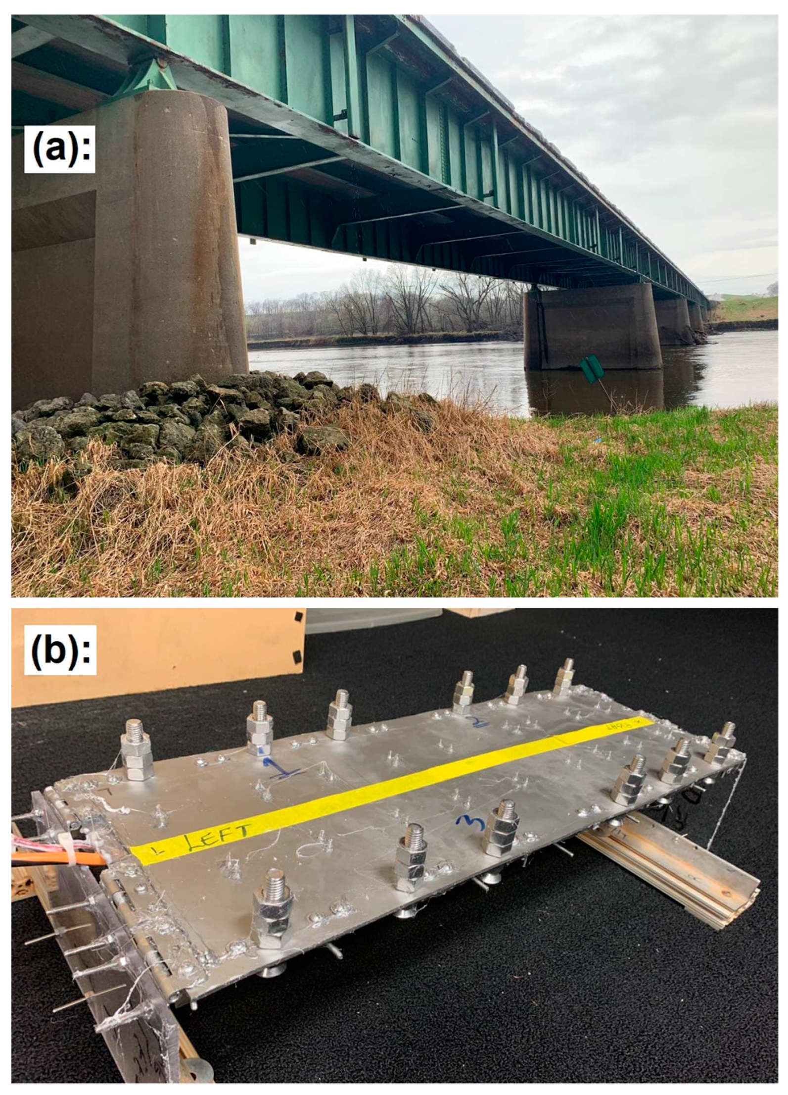
Figure 2.
FEM of the small-scale bridge and its dominant modes in the dry condition: (a) undeformed FEM; (b) 1st mode shape; (c) 4th mode shape; (d) 17th mode shape. The model is colored by normalized displacement magnitude.
Figure 2.
FEM of the small-scale bridge and its dominant modes in the dry condition: (a) undeformed FEM; (b) 1st mode shape; (c) 4th mode shape; (d) 17th mode shape. The model is colored by normalized displacement magnitude.
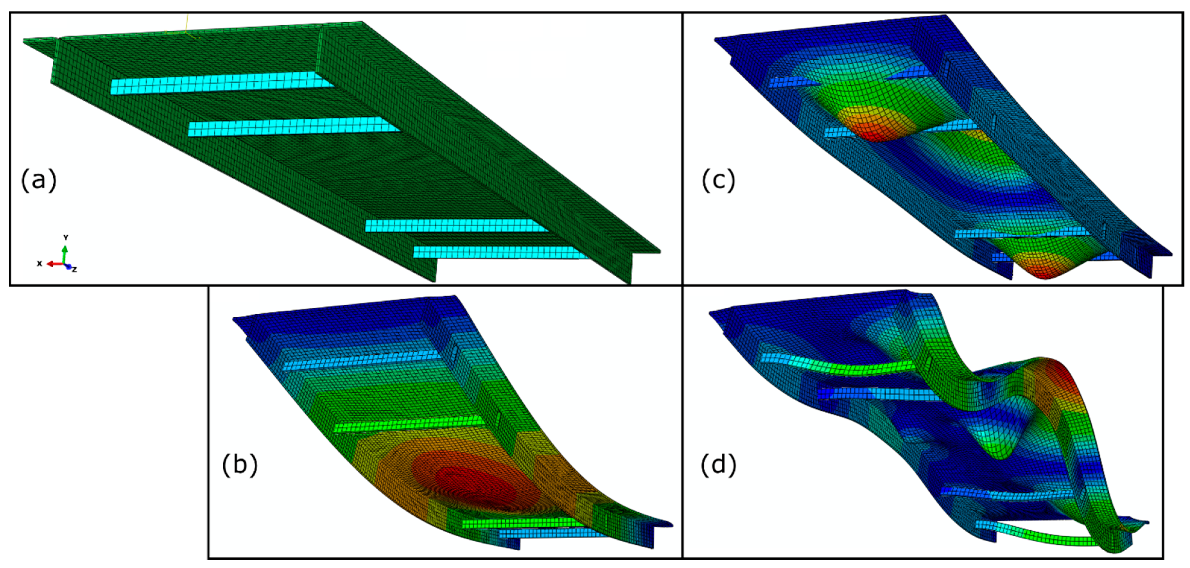
Figure 3.
FEM of the small-scale bridge and its dominant modes in the semi-inundated condition: (a) undeformed FEM; (b) 1st mode shape; (c) 4th mode shape; (d) 17th mode shape.
Figure 3.
FEM of the small-scale bridge and its dominant modes in the semi-inundated condition: (a) undeformed FEM; (b) 1st mode shape; (c) 4th mode shape; (d) 17th mode shape.
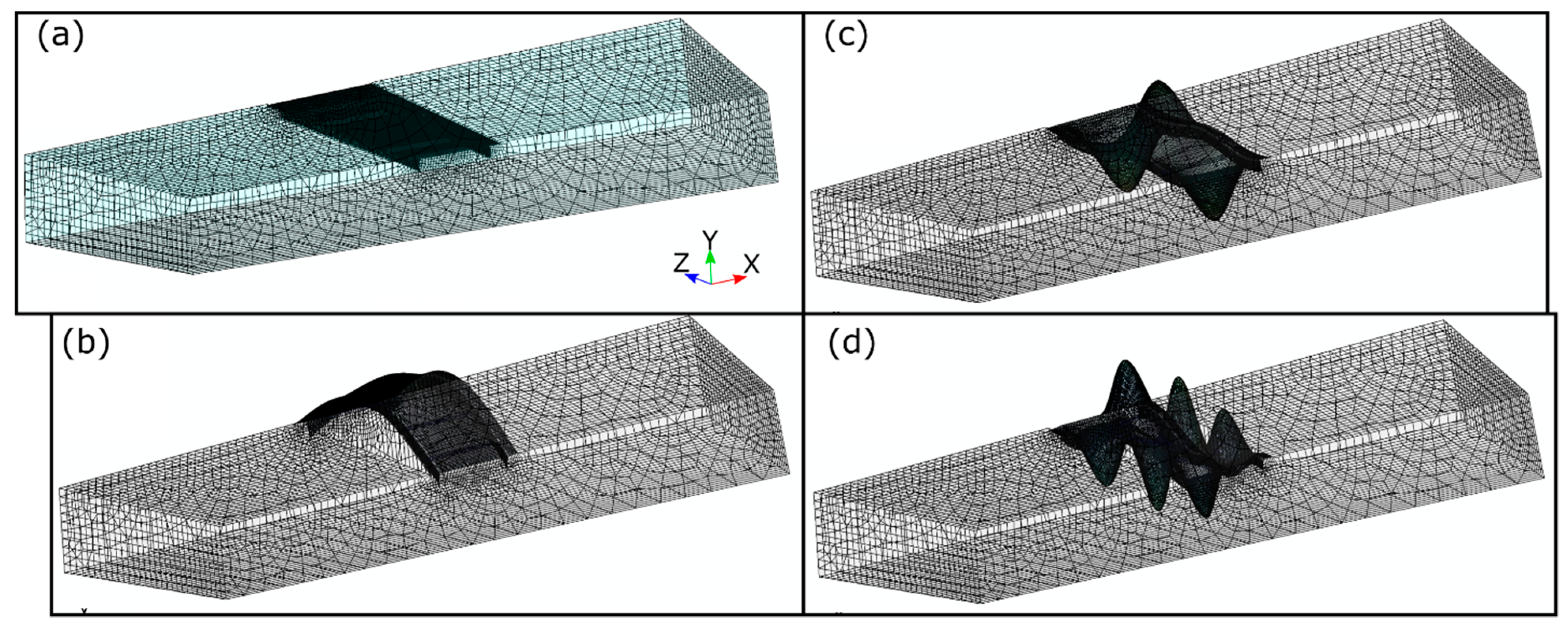
Figure 4.
FEM of the small-scale bridge and its dominant modes in the fully inundated condition: (a) undeformed FEM; (b) 1st mode shape; (c) 4th mode shape; (d) 17th mode shape.
Figure 4.
FEM of the small-scale bridge and its dominant modes in the fully inundated condition: (a) undeformed FEM; (b) 1st mode shape; (c) 4th mode shape; (d) 17th mode shape.

Figure 5.
FEM of the full-scale bridge and its dominant modes in the dry condition: (a) undeformed FEM; (b) 1st mode shape; (c) 4th mode shape; (d) 9th mode shape. The model is colored by normalized displacement magnitude.
Figure 5.
FEM of the full-scale bridge and its dominant modes in the dry condition: (a) undeformed FEM; (b) 1st mode shape; (c) 4th mode shape; (d) 9th mode shape. The model is colored by normalized displacement magnitude.

Figure 6.
FEM of the full-scale bridge and its dominant modes in the semi-inundated condition: (a) undeformed FEM; (b) 1st mode shape; (c) 4th mode shape; (d) 9th mode shape.
Figure 6.
FEM of the full-scale bridge and its dominant modes in the semi-inundated condition: (a) undeformed FEM; (b) 1st mode shape; (c) 4th mode shape; (d) 9th mode shape.

Figure 7.
FEM of the full-scale bridge and its dominant modes in the fully inundated condition: (a) undeformed FEM; (b) 1st mode shape; (c) 4th mode shape; (d) 9th mode shape.
Figure 7.
FEM of the full-scale bridge and its dominant modes in the fully inundated condition: (a) undeformed FEM; (b) 1st mode shape; (c) 4th mode shape; (d) 9th mode shape.
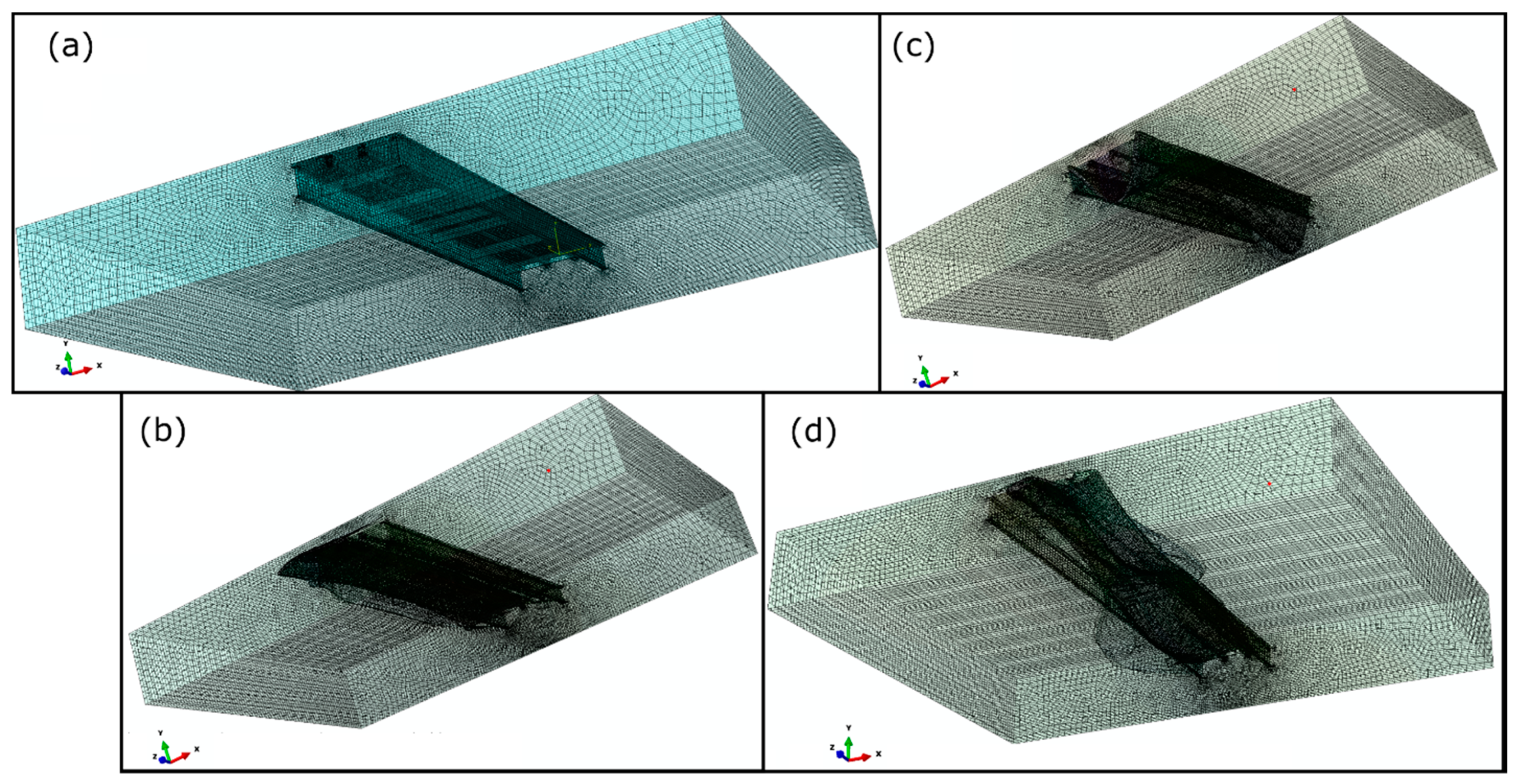
Figure 8.
Experimental setup of the small-scale bridge in the flume laboratory in progressive flood stages: (a) dry; (b) semi-inundated; (c) fully inundated.
Figure 8.
Experimental setup of the small-scale bridge in the flume laboratory in progressive flood stages: (a) dry; (b) semi-inundated; (c) fully inundated.
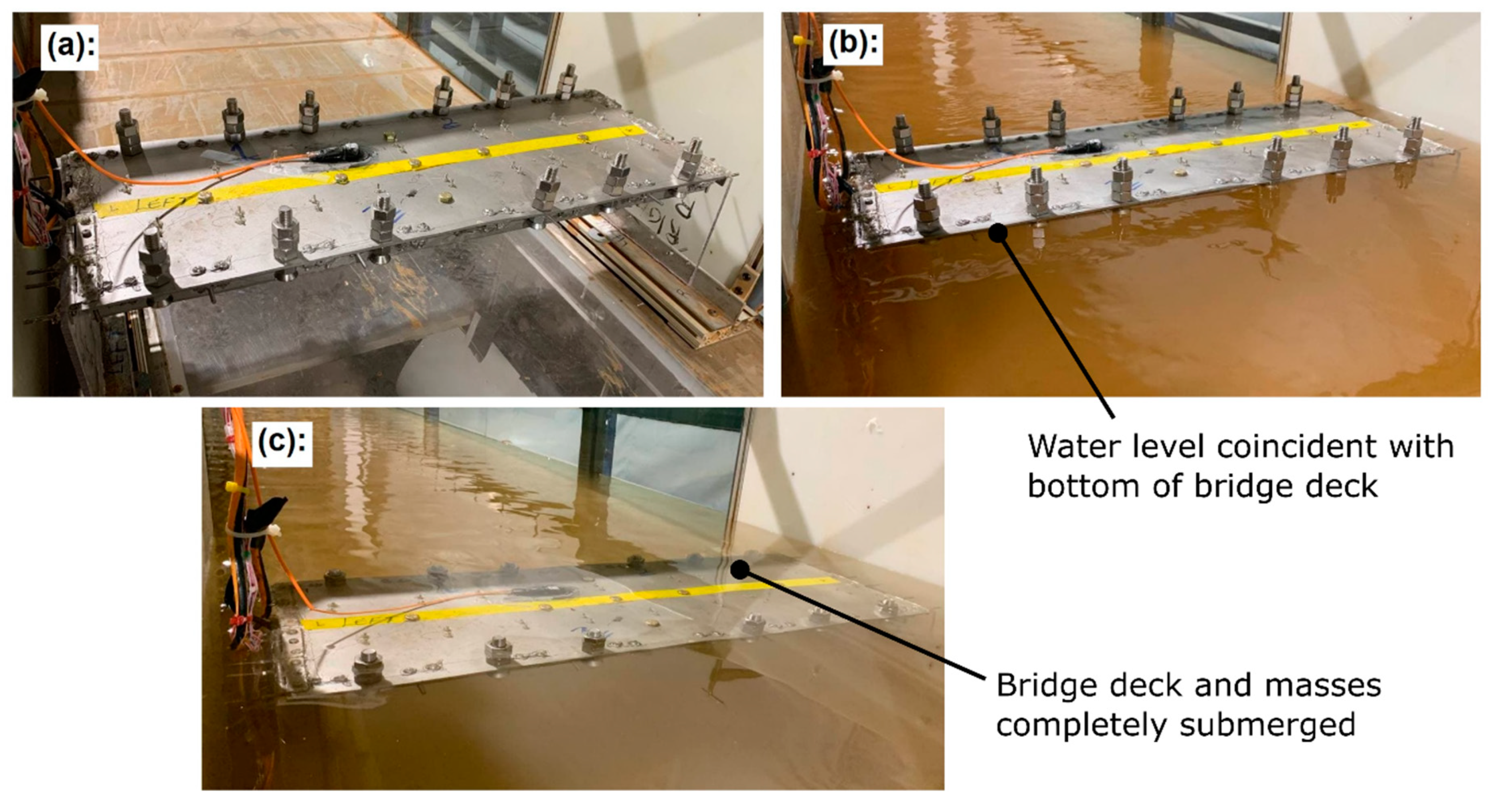
Figure 9.
Acceleration data from experimental setup of the small-scale model for NFs extraction by FDD and SVD. The first column (a,d,g) shows the acceleration signals for the dry, semi-inundated, and fully inundated cases, respectively; the second column (b,e,h) shows the acceleration PSD signals for the dry, semi-inundated, and fully inundated cases, respectively; the third column (c,f,i) shows the acceleration SVD signals with detected system poles indicated by vertical dashed lines, passing through the peaks of the SVD signals, for the dry, semi-inundated, and fully inundated cases, respectively.
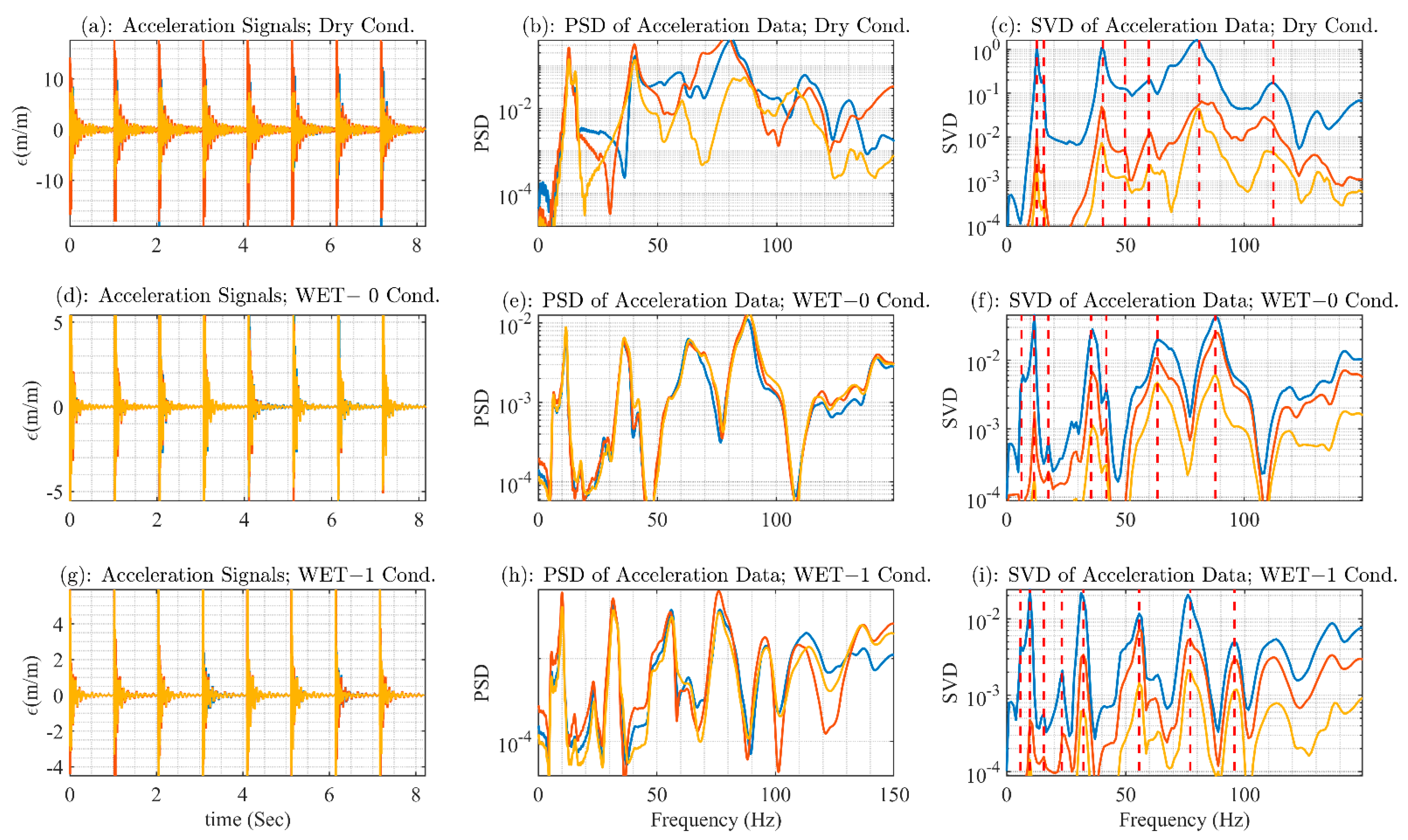
Figure 10.
Strain data from experimental setup of the small-scale model for NFs extraction by FDD and SVD. The first column (a,d,g) shows the strain signals for the dry, semi-inundated, and fully inundated cases, respectively; the second column (b,e,h) shows the strain PSD signals for the dry, semi-inundated, and fully inundated cases, respectively; the third column (c,f,i) shows the strain SVD signals with detected system poles indicated by vertical dashed lines, passing through the peaks of the SVD signals, for the dry, semi-inundated, and fully inundated cases, respectively.
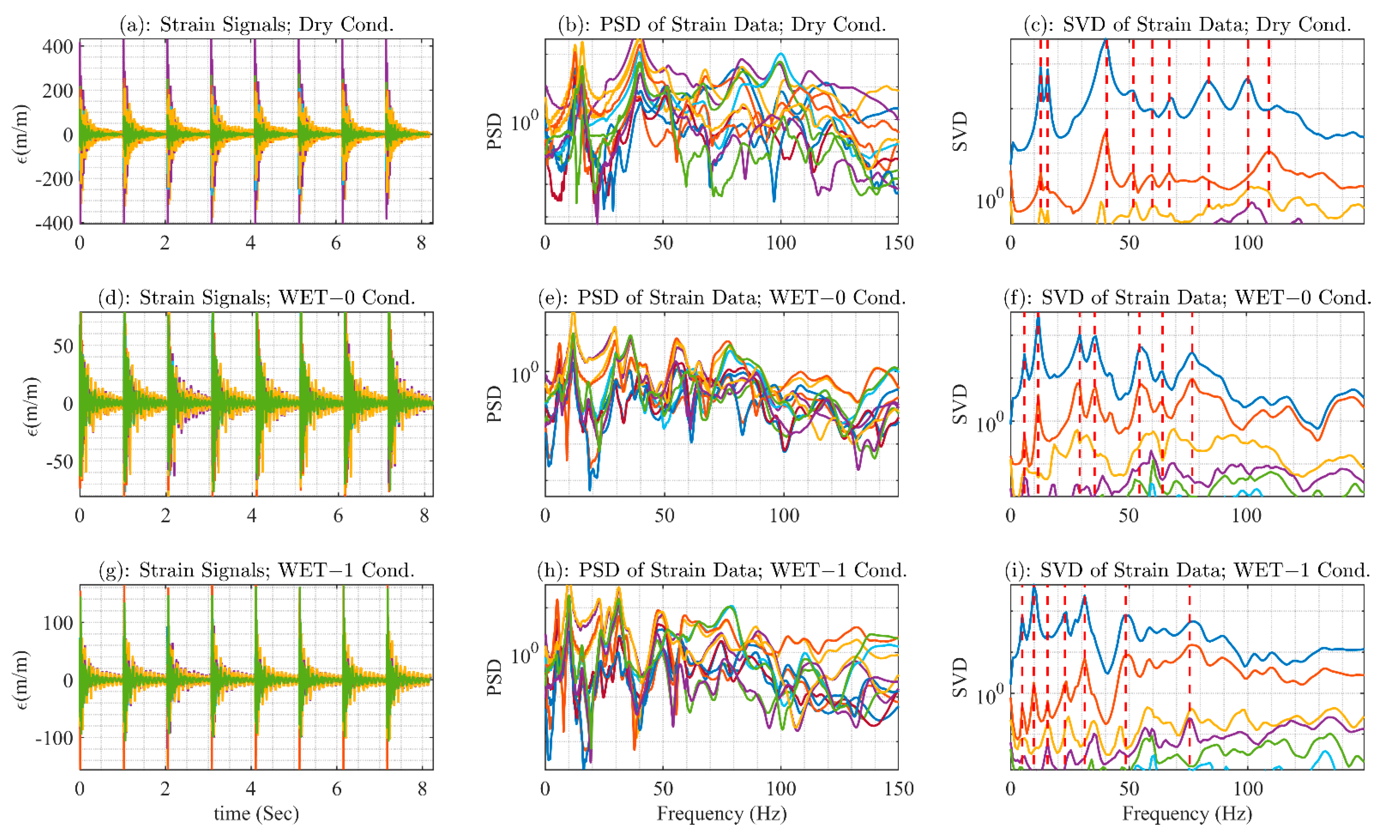
Figure 11.
Comparison of NFs of the small-scale experimental model under various flood stages, extracted from acceleration and strain signals.
Figure 11.
Comparison of NFs of the small-scale experimental model under various flood stages, extracted from acceleration and strain signals.

Table 1.
Physical properties of materials used for FEM-CAS simulations.
| Characteristic | Nominal Values | |||||
|---|---|---|---|---|---|---|
| Material | Air | Water | Steel | Lexan | Aluminum | Concrete |
| 1.21 | 998 | 7830 | 1060 | 2700 | 2300 | |
| Poisson’s ratio | - | - | 0.3 | 0.38 | 0.33 | 0.2 |
| - | - | 193 | 2.32 | 70 | 22 | |
| 1.39 × 10⁻⁴ | 2.19 | 160 | 5.8 | 107.8 | 31.5 | |
| 340 | 1481.3 | 4520 | 2350 | 6320 | 3700 | |
Table 2.
Experimental and numerical NFs, effective modal mass, and HAM for the small-scale model.
| Dry Condition | Semi-Inundation | Full Inundation | ||||||
|---|---|---|---|---|---|---|---|---|
| Dominant modes | NFs (Hz) | NFs (Hz) | HAM (kg) | NFs (Hz) | HAM (kg) | |||
| 1st mode | 12.43 (12.7) | 4.1247 (81%) | 5.9 (6.3) | 52.5 | 14.2 (+280%) | 5.1 (5.8) | 59 | 20.3 (+403%) |
| 4th mode | 38.91 (40.5) | 0.29 (5.7%) | 32.7 (35.6) | 15.9 | 0.12 (+2.3%) | 29.7 (32.3) | 24 | 0.2 (+4.1%) |
| 17th mode | 165.51 | 0.19 (3.7%) | 103.91 | 37.2 | 0.29 (+5.7%) | 85.1 | 49 | 0.52 (+10%) |
Table 3.
Experimental and numerical NFs, effective modal mass, and HAM for the full-scale model.
| Dry Condition | Semi-Inundation | Full Inundation | ||||||
|---|---|---|---|---|---|---|---|---|
| Dominant modes | NFs (Hz) | (Metric ton) | NFs (Hz) | HAM (metric ton) | NFs (Hz) | HAM (metric ton) | ||
| 1st mode | 2.57 | 410 (72%) | 1.03 | 60 | 2142 (+375%) | 0.85 | 67 | 3338 (+585%) |
| 4th mode | 3.52 | 34.8 (6.1%) | 1.64 | 53.4 | 125 (+34) | 1.16 | 67 | 285 (+50%) |
| 9th mode | 7.15 | 56 (9.8%) | 4.38 | 38.7 | 93 (+16) | 3.34 | 53 | 200 (+35%) |
Publisher’s Note: MDPI stays neutral with regard to jurisdictional claims in published maps and institutional affiliations. |
© 2022 by the authors. Licensee MDPI, Basel, Switzerland. This article is an open access article distributed under the terms and conditions of the Creative Commons Attribution (CC BY) license (https://creativecommons.org/licenses/by/4.0/).
Share and Cite
MDPI and ACS Style
Karimpour, A.; Rahmatalla, S.; Harwood, C. Effect of Directional Added Mass on Highway Bridge Response during Flood Events. Infrastructures 2022, 7, 42. https://doi.org/10.3390/infrastructures7030042
AMA Style
Karimpour A, Rahmatalla S, Harwood C. Effect of Directional Added Mass on Highway Bridge Response during Flood Events. Infrastructures. 2022; 7(3):42. https://doi.org/10.3390/infrastructures7030042
Chicago/Turabian StyleKarimpour, Ali, Salam Rahmatalla, and Casey Harwood. 2022. "Effect of Directional Added Mass on Highway Bridge Response during Flood Events" Infrastructures 7, no. 3: 42. https://doi.org/10.3390/infrastructures7030042