
Observed Seismic Behavior of a HDRB and SD Isolation System under Far Fault Earthquakes

 , , and
Abstract
:1. Introduction
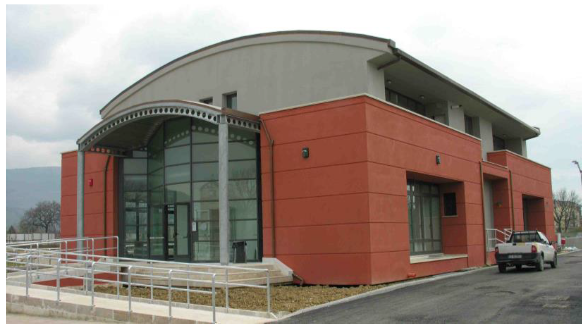
2. The Forest Ranger Building and the Monitoring System
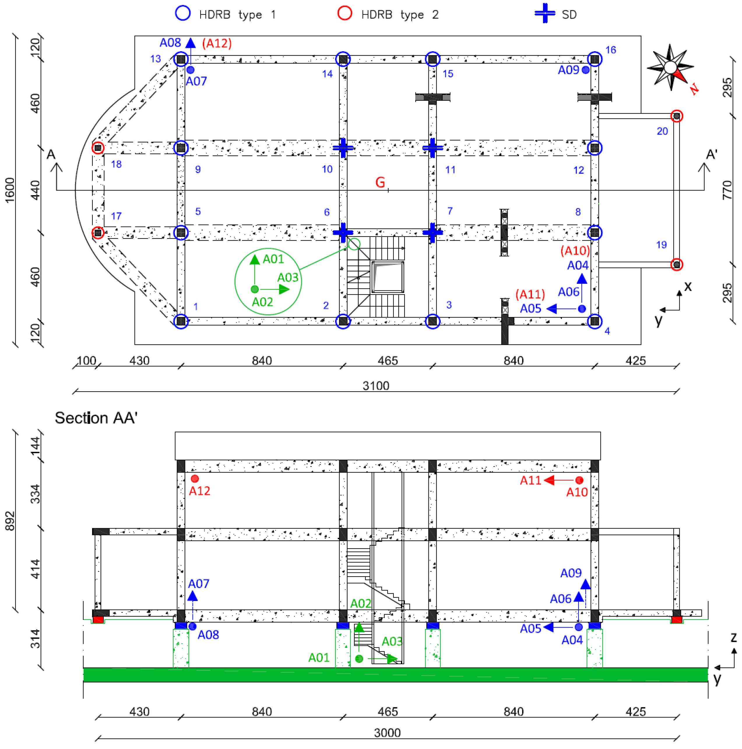
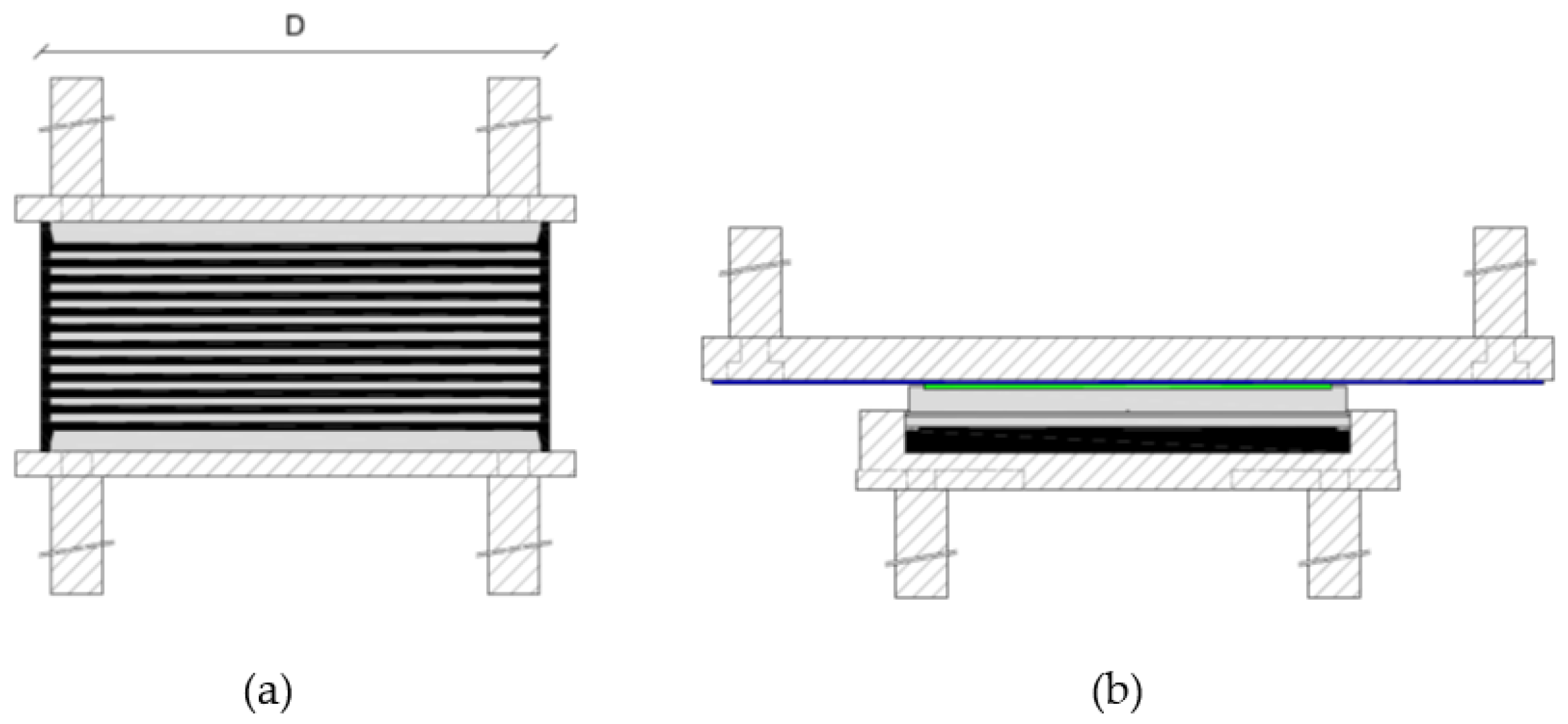
2.1. The Building and the Isolation System
- 12 HDRBs of Type 1, located along the perimeter of the main rectangular portion;
- 4 flat slider devices (SD) with a lubricated steel-PTFE (polytetrafluoroethylene) interface, having a nominal friction factor of 1.0%, located at the internal column of the main rectangular portion;
- 4 HDRBs of Type 2, located at the columns external to the main portion.
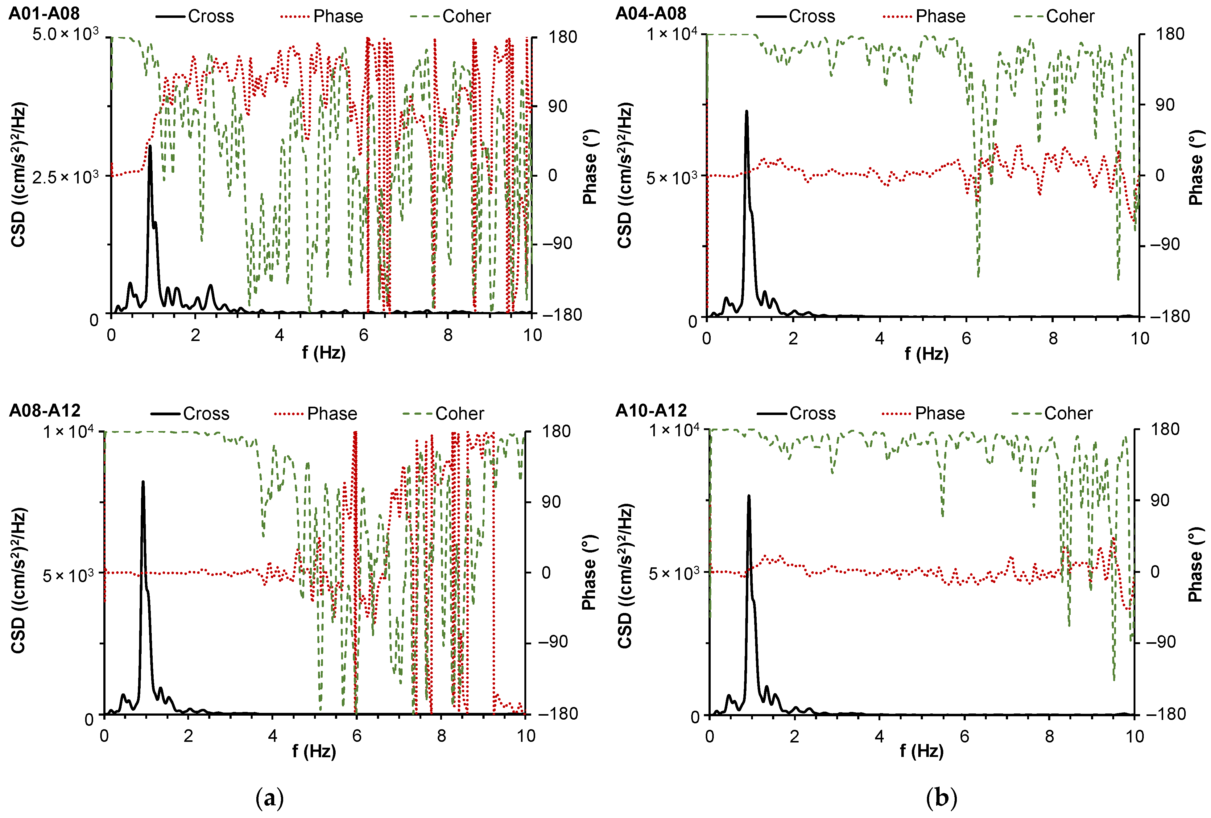
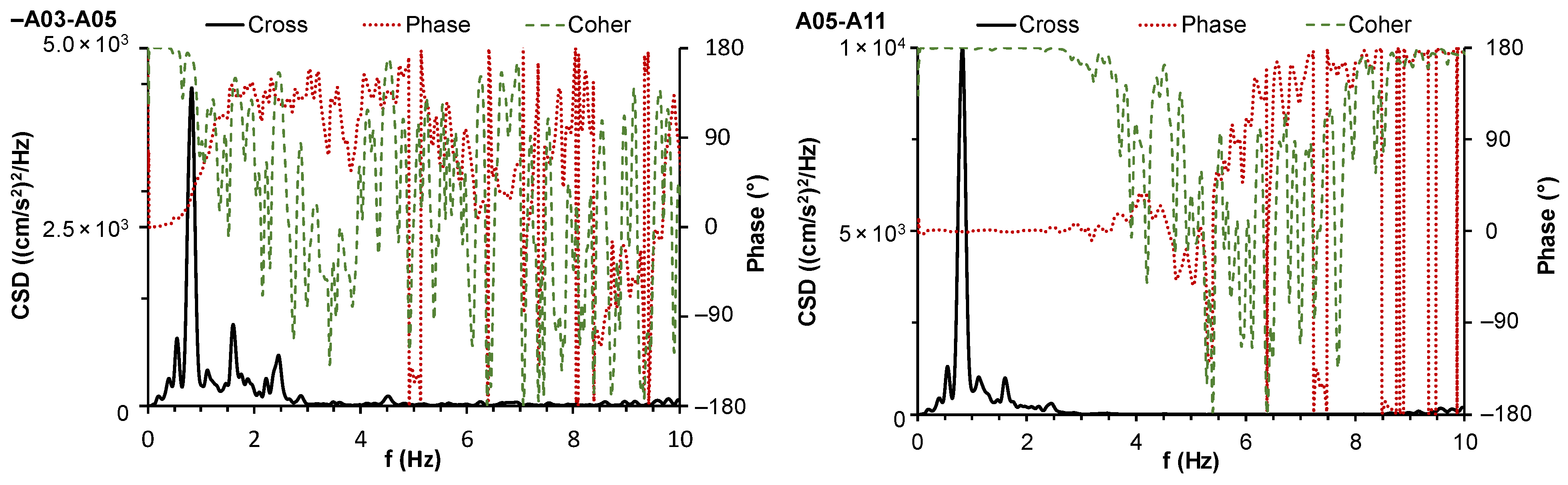
2.2. Behavior under Ambient Vibrations
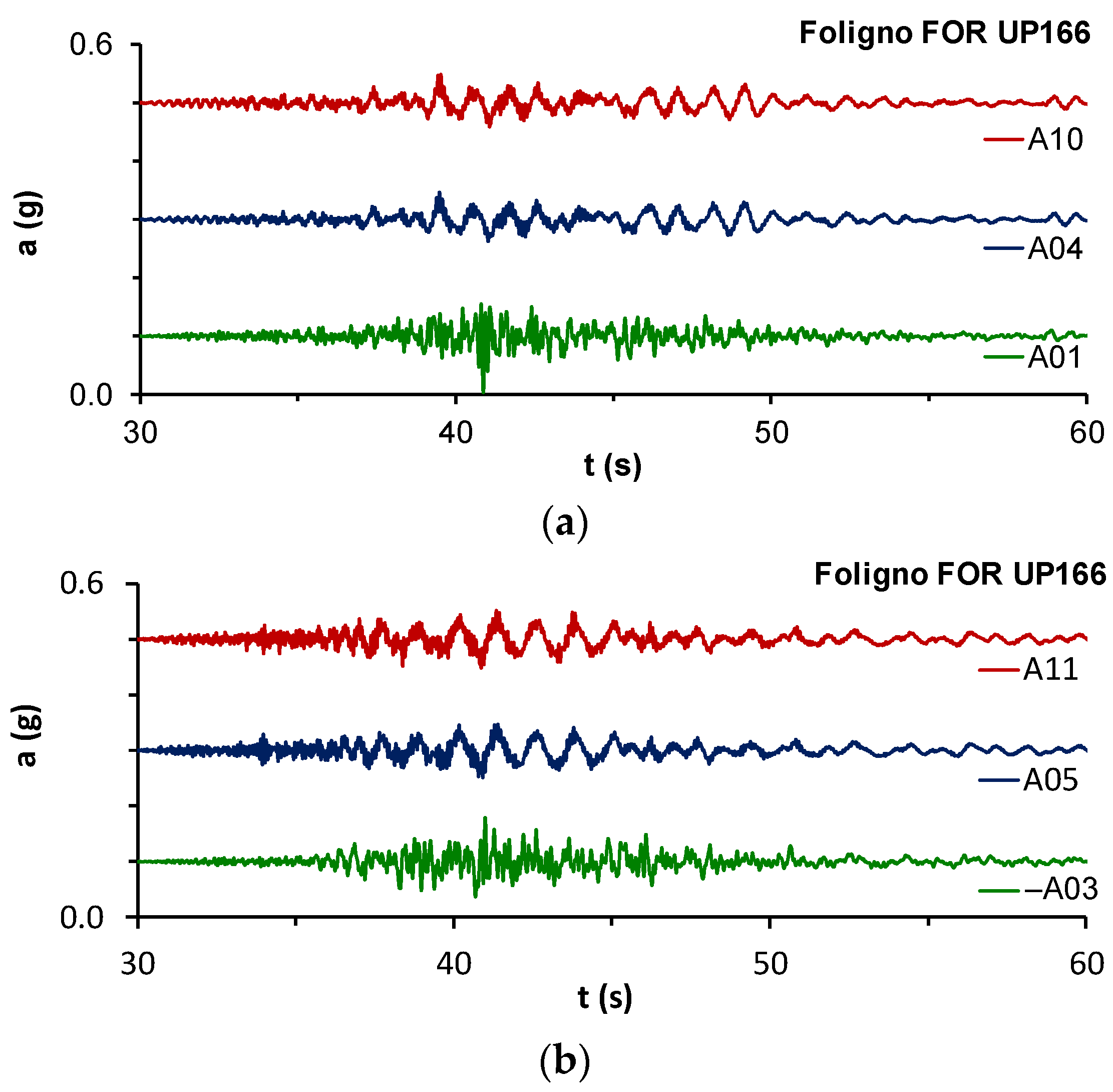
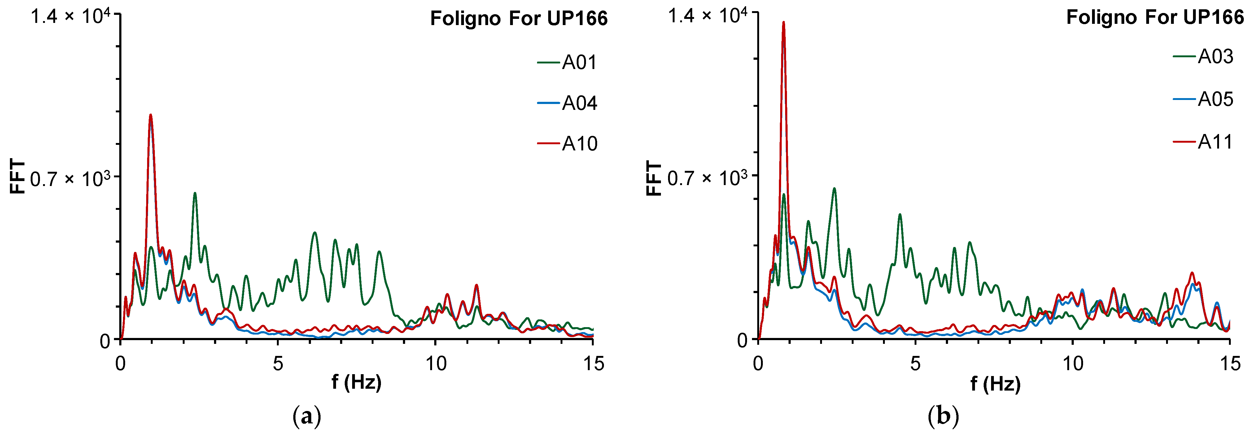
2.3. The Permanent Accelerometer Network
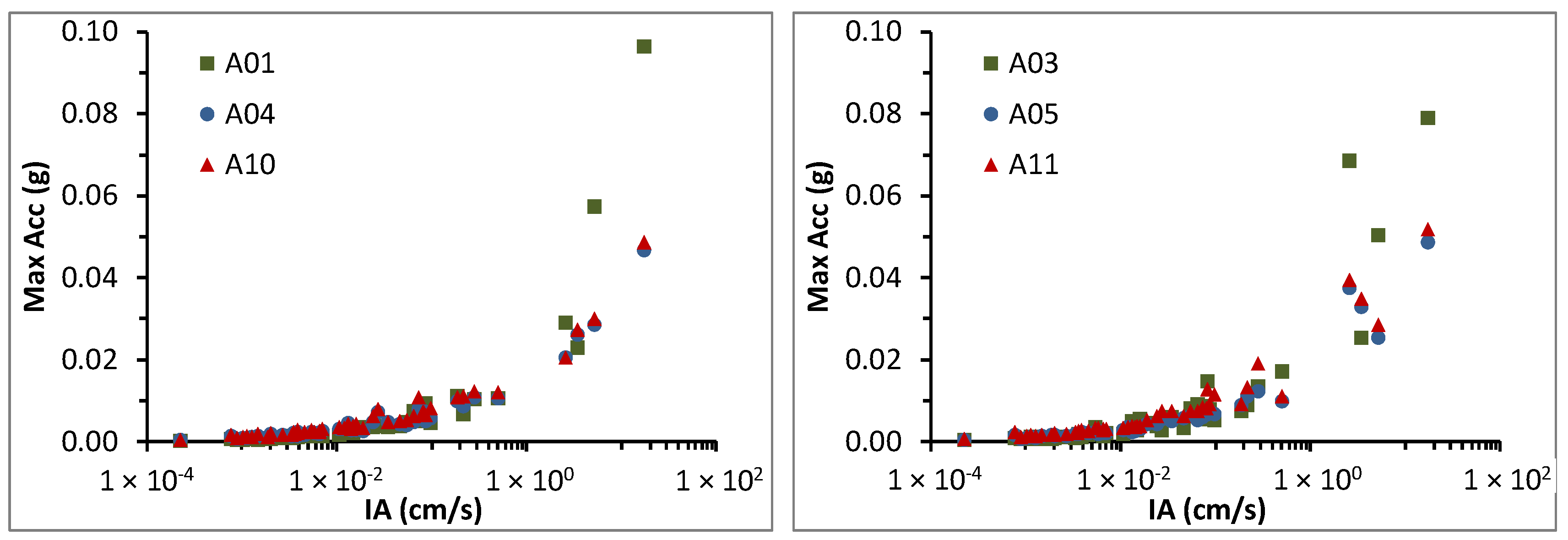
- Three accelerometers, A01, A02 and A03, are at the basement (level 0, L0) in x, vertical and y direction, respectively;
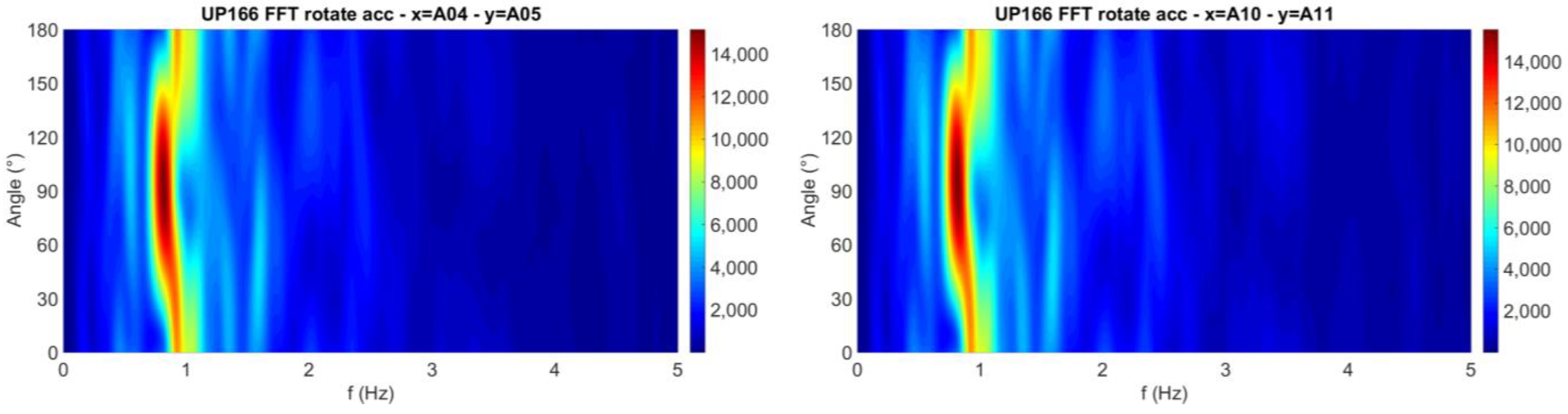
- Five accelerometers are on the slab above the isolation interface (level 1, L1), as follows: A04 and A08 in x direction, A05 in y direction, and A06, A07 and A09 in the vertical direction;
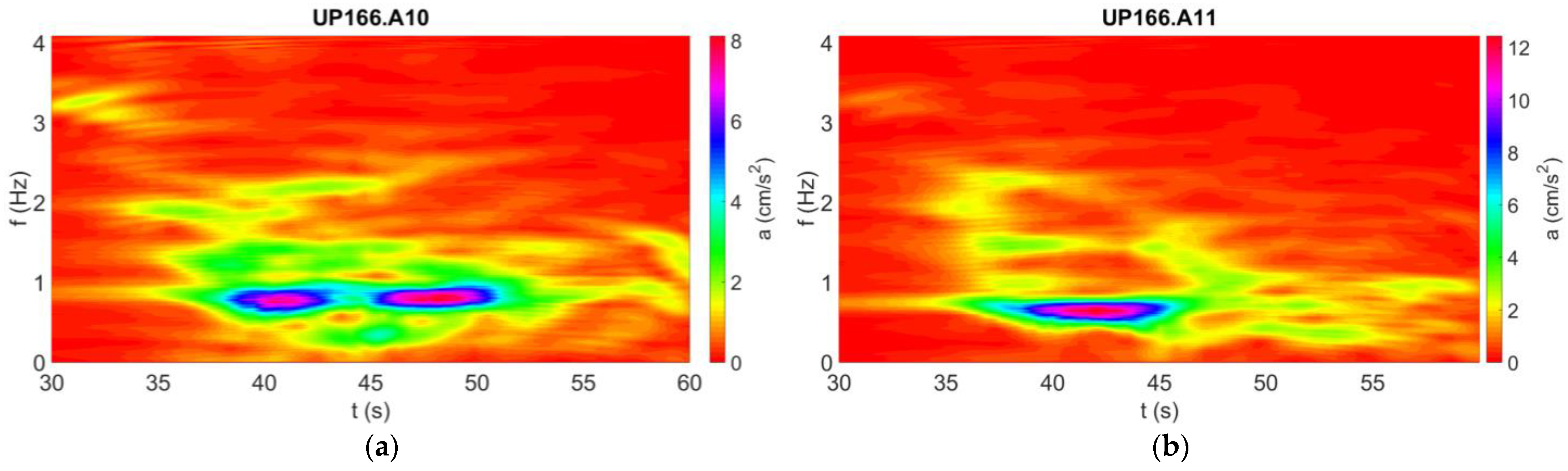
- Three accelerometers are at the top of the building (level 2, L2), as follows: A10 and A12 in x direction and A11 in y direction.
3. Observed Seismic Behavior
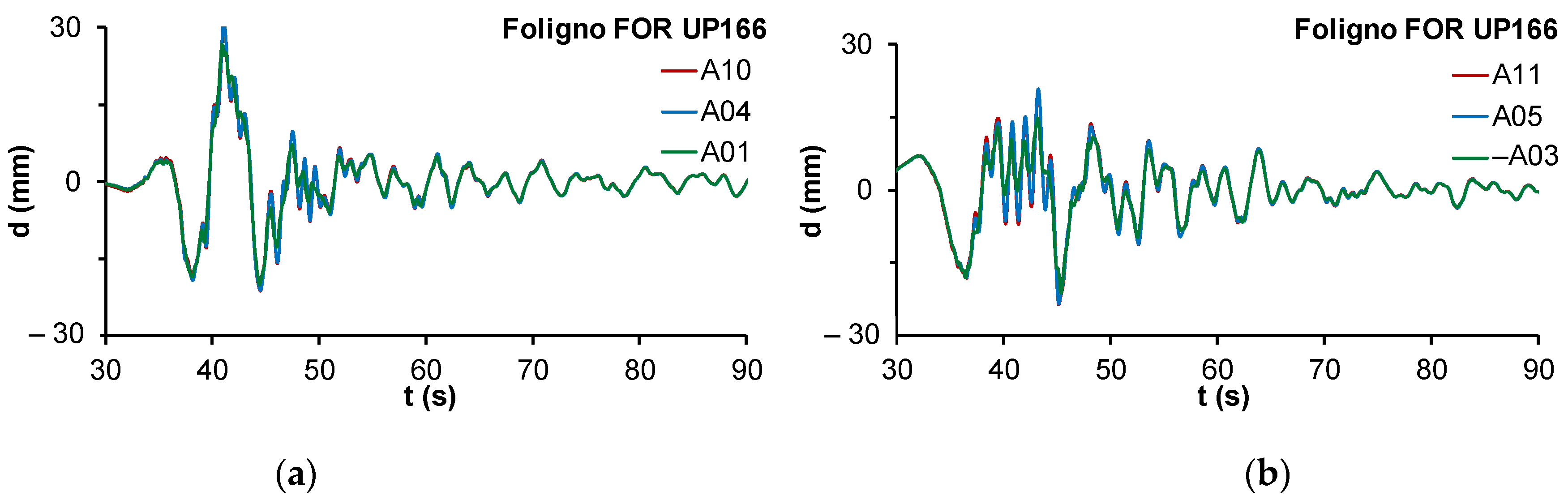
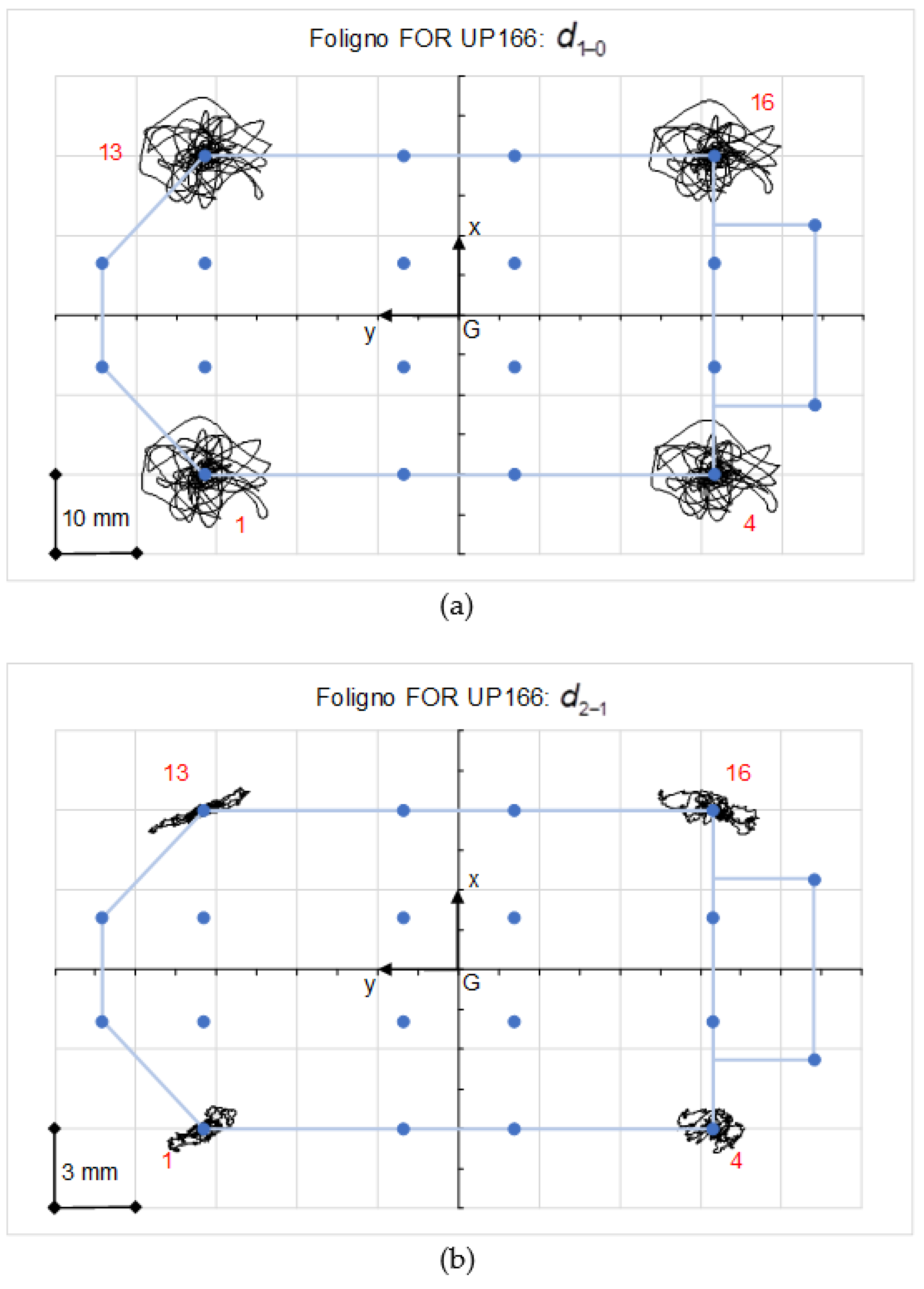
3.1. The 30 October 2016 Norcia Earthquake
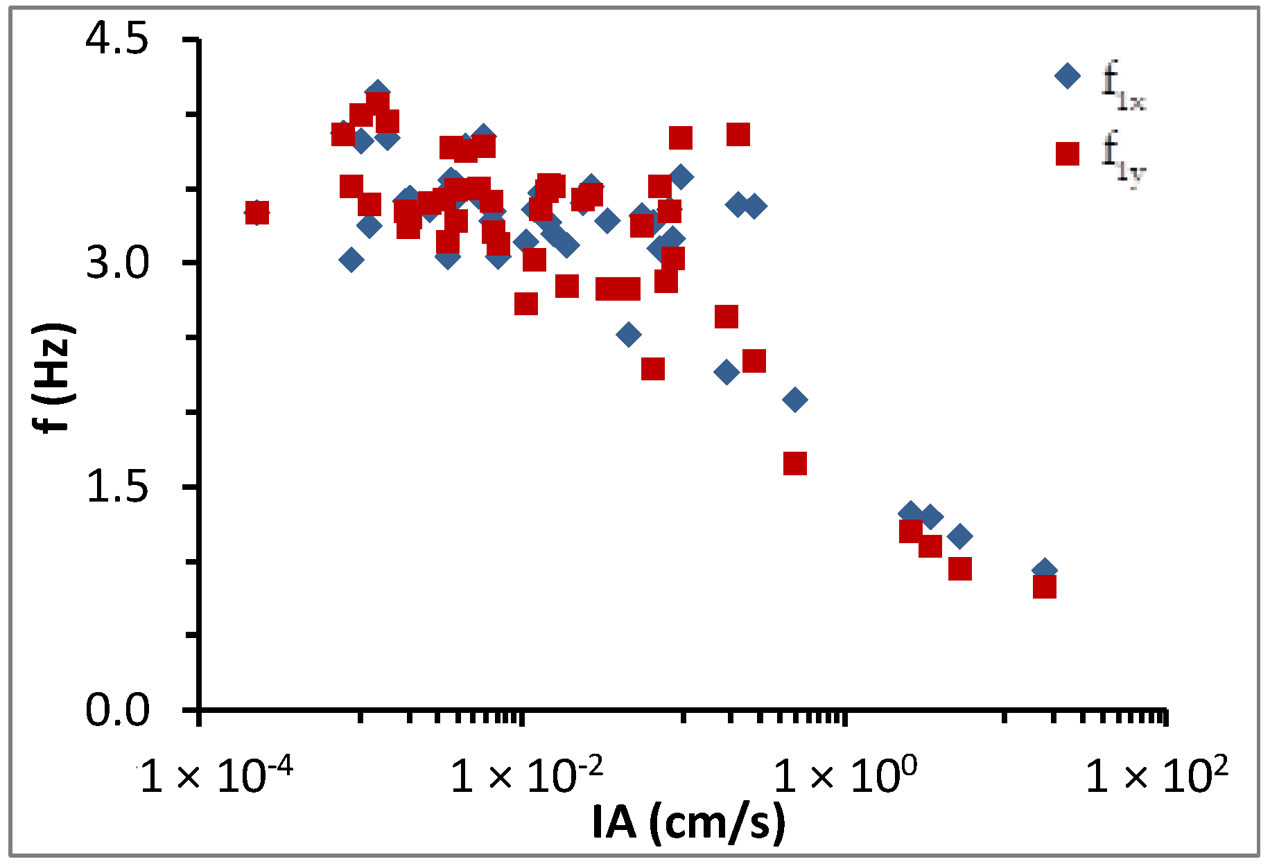
3.2. Comparison of the Structure Behavior under Different Seismic Events
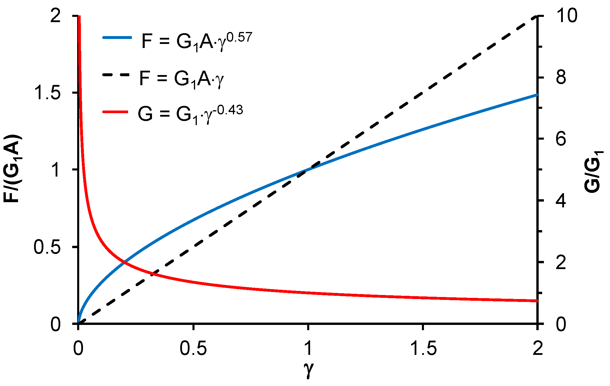
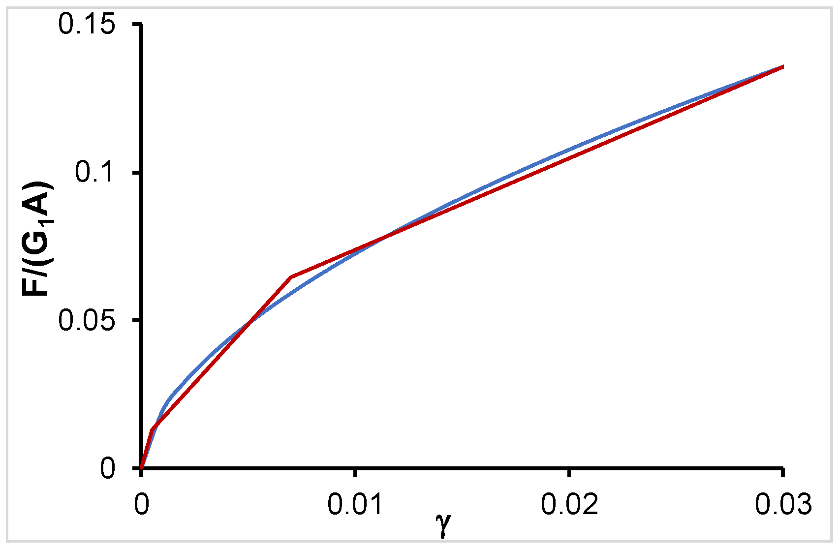
4. Non-Linear Modelling of the Isolation System
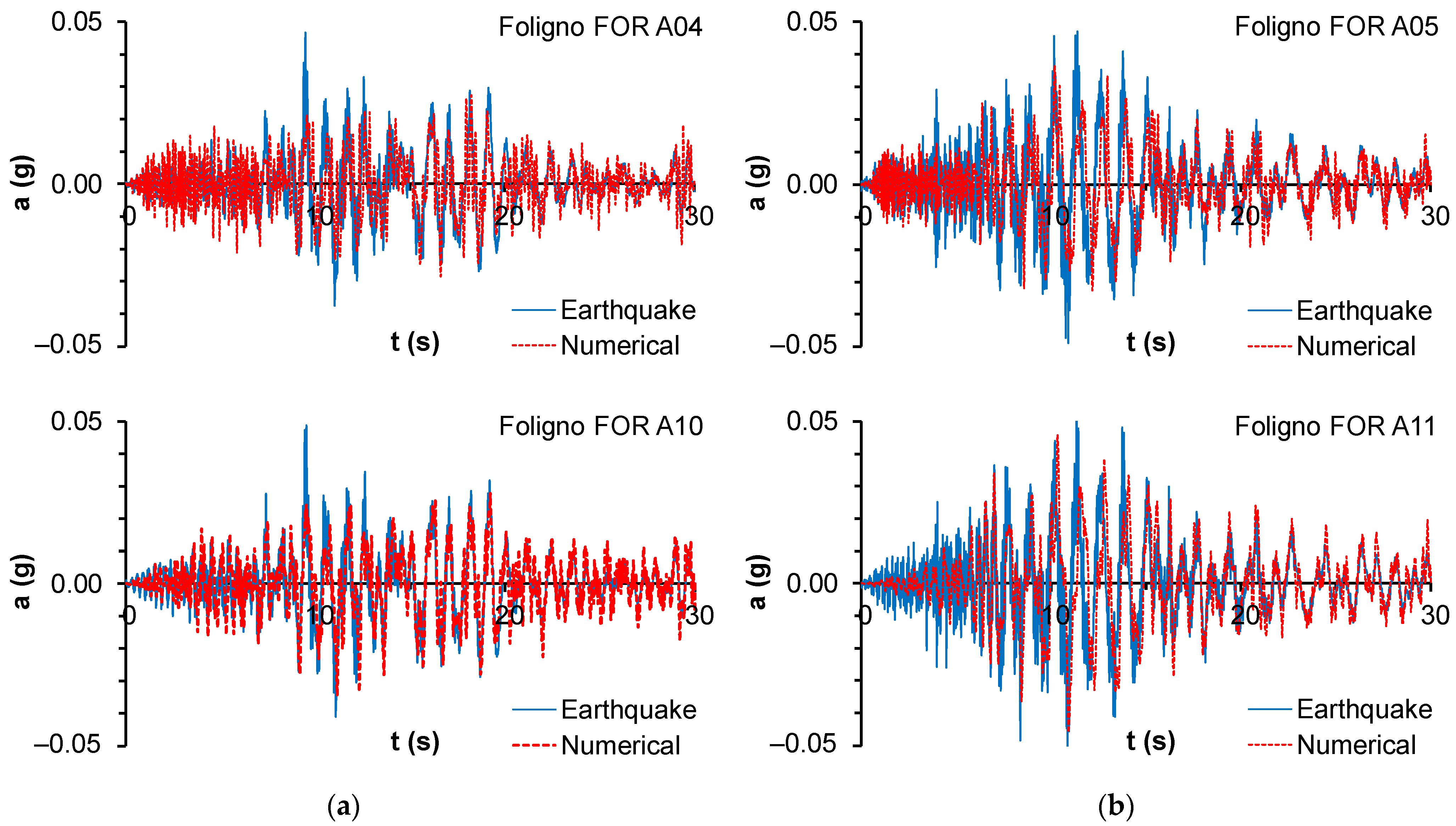
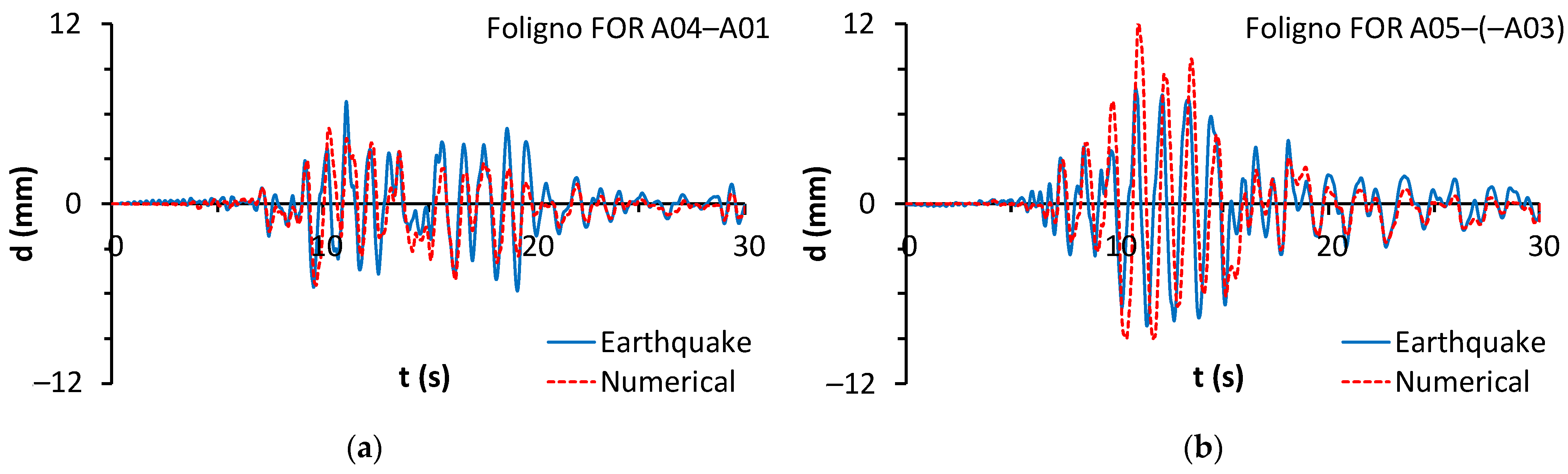
5. Comparison between the Observed Behavior and the Numerical Analysis
6. Conclusions
- The resonance frequencies varied significantly with the energy at the site of the building and approached to the resonance frequencies of the superstructure for the lowest energy events.
- As a result, there was no suitable decoupling of motion in some cases. This occurrence must be accounted for in the design of the isolation system and to evaluate the seismic actions in the superstructure.
- The contribution of sliding devices was very important for the onset of motion under low energy earthquake. Actually, the isolation system was not put in action under very low energy events but only when the maximum friction forces in the sliding devices were not sufficient to face the seismic actions.
- The contribution of the sliding devices significantly influenced the amplitude of vibrations and damping.
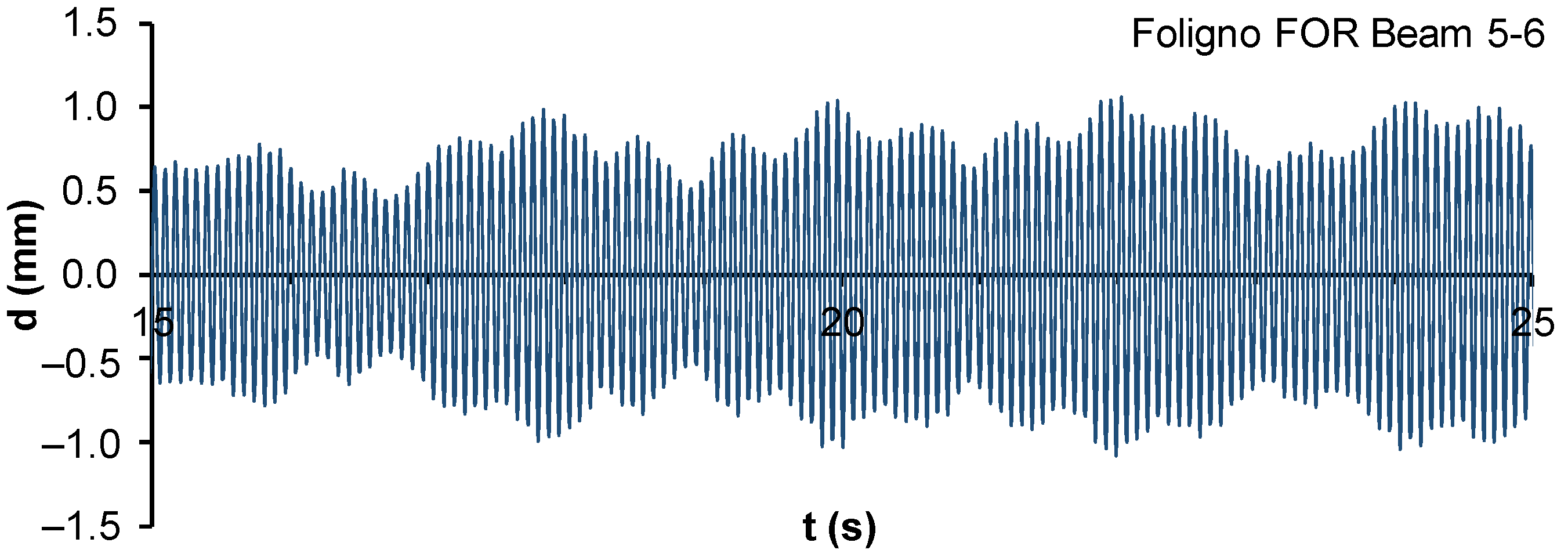
- The analysis of the relative vertical displacements between the beams around the damaged partition walls pointed out vibrations at high frequency and amplitudes greater than 2.0 mm. These acted in conjunction with the horizontal vibrations and can justify the observed small cracks.
Author Contributions
Funding
Conflicts of Interest
References
- Clemente, P. Seismic isolation: Past, present and the importance of SHM for the future. J. Civ. Struct. Heal. Monit. 2017, 7, 217–231. [Google Scholar] [CrossRef]
- Calvi, P.M.; Calvi, G.M. Historical development of friction-based seismic isolation systems. Soil Dyn. Earthq. Eng. 2018, 106, 14–30. [Google Scholar] [CrossRef]
- Naeim, F.; Kelly, J.M. Design of Seismic Isolated Structures: From Theory to Practice; John Wiley & Sons Inc.: Hoboken, NJ, USA, 1999. [Google Scholar] [CrossRef]
- Skinner, R.I.; Robinson, W.H.; McVerry, G.H. An introduction to Seismic Isolation. DSIR Physical Sciences; John Wiley & Sons Inc.: Wellington, New Zealand, 1993. [Google Scholar]
- Clemente, P.; Martelli, A. Seismically isolated buildings in Italy: State-of-the-art review and applications. Soil Dyn. Earthq. Eng. 2019, 119, 471–487. [Google Scholar] [CrossRef]
- Bongiovanni, G.; Buffarini, G.; Clemente., P.; Saitta, F.; Tripepi, C. Retrofit of existing buildings with seismic isolation: Design issues and applications. In Proceedings of the 16th World Conference on Seismic Isolation, Energy Dissipation and Active Vibration Control of Structures, 16WCSI, St. Petersburg, FL, USA, 1–6 July 2019; pp. 111–122. [Google Scholar] [CrossRef]
- Saitta, F.; Clemente, P.; Buffarini, G.; Bongiovanni, G. Vulnerability Analysis and Seismic Retrofit of a Strategic Building. J. Perform. Constr. Facil. 2017, 31, 04016085. [Google Scholar] [CrossRef]
- Çelebi, M. Successful performance of a base-isolated hospital buildings during the 17 January 1995 Northridge earthquake. Struct. Des. Tall Build. 1996, 5, 95–109. [Google Scholar] [CrossRef]
- Nagarajaiah, S.; Xiaohong, S. Response of Base-Isolated USC Hospital Building in Northridge Earthquake. J. Struct. Eng. 2000, 126, 1177–1186. [Google Scholar] [CrossRef]
- Nagarajaiah, S.; Sun, X. Base-Isolated FCC Building: Impact Response in Northridge Earthquake. J. Struct. Eng. 2001, 127, 1063–1075. [Google Scholar] [CrossRef] [Green Version]
- Loh, C.-H.; Weng, J.-H.; Chen, C.-H.; Lu, K.-C. System identification of mid-story isolation building using both ambient and earthquake response data. Struct. Control. Health Monit. 2011, 20, 139–155. [Google Scholar] [CrossRef]
- Matsuda, K.; Kasai, K.; Yamagiwa, H.; Sato, D. Responses of base-isolated buildings in Tokyo during the 2011 Great East Japan Earthquake. In Proceedings of the 15th World Conf. on Earthquake Engineering (15WCEE), Lisbon, Portugal, 24–28 September 2012. [Google Scholar]
- Siringoringo, D.M.; Fujino, Y. Seismic response analyses of an asymmetric base-isolated building during the 2011 Great East Japan (Tohoku) Earthquake. Struct. Control. Health Monit. 2014, 22, 71–90. [Google Scholar] [CrossRef]
- Zhou, F.L.; Tan, P.; Heisha, W.; Huan, X.Y. Progress and application of seismic isolation, energy dissipation and control in civil and industrial structures and design codes in China. In Proceedings of the 14th World Conf. on Seismic Isolation, Energy Dissipation and Active Vibration Control of Structures (14WCSI), San Diego, CA, USA, 9–11 September 2015. [Google Scholar]
- Zhou, C.; Chase, J.G.; Rodgers, G.W.; Kuang, A.; Gutschmidt, S.; Xu, C. Performance evaluation of CWH base isolated building during two major earthquakes in Christchurch. Bull. N. Z. Soc. Earthq. Eng. 2015, 48, 264–273. [Google Scholar] [CrossRef] [Green Version]
- Takayama, M.; Morita, K. Observed performance of seismically isolated buildings during 2016 Kumamoto Earthquake in Japan. In Proceedings of the 17th World Conference on Earthquake Engineering (17WCEE), Sendai, Japan, 28 September–2 October 2021. Paper N° C000234. [Google Scholar]
- Martelli, A.; Clemente, P.; De Stefano, A.; Forni, M.; Salvatori, A. Recent Development and Application of Seismic Isolation and Energy Dissipation and Conditions for Their Correct Use. In Geotechnical, Geological and Earthquake Engineering; Springer: Berlin/Heidelberg, Germany, 2014; Volume 34, pp. 449–488. [Google Scholar] [CrossRef]
- Clemente, P.; Buffarini, G. Base isolation: Design and optimization criteria. SIAPS 2010, 1, 17–40. [Google Scholar] [CrossRef] [Green Version]
- Clemente, P.; Bontempi, F.; Boccamazzo, A. Seismic Isolation in Masonry Buildings: Technological and economic issues. In Brick and Block Masonry: Trends, Innovation and Challenges, Proceedings of the 6th International Conference (IB2MAC), Padua, Italy, 26–30 Jun 2016; Modena, C., da Porto, F., Valluzzi, M.R., Eds.; Taylor & Francis Group: London, UK, 2016; pp. 2207–2215. ISBN 978-1-138-02999-6. [Google Scholar]
- Tripepi, C.; Clemente, P. Graphic Procedure for the Optimum Design of Elastomeric Isolators. Pract. Period. Struct. Des. Constr. 2021, 26, 04020058. [Google Scholar] [CrossRef]
- Saitta, F.; Clemente, P.; Buffarini, G.; Bongiovanni, G.; Salvatori, A.; Grossi, C. Base Isolation of Buildings with Curved Surface Sliders: Basic Design Criteria and Critical Issues. Adv. Civ. Eng. 2018, 2018, 1–14. [Google Scholar] [CrossRef]
- Clemente, P.; Bongiovanni, G.; Buffarini, G.; Saitta, F.; Scafati, F. Monitored Seismic Behavior of Base Isolated Buildings in Italy. In Seismic Structural Health Monitoring, Springer Tracts in Civil Engineering; Limongelli, M., Celebi, M., Eds.; Springer: Cham, Switzerland, 2019; pp. 115–137. [Google Scholar] [CrossRef]
- Ormando, C.; Clemente, P.; Ianniruberto, U.; Scafati, F. Onset of Motion of Curved Surface Sliders Used in Seismic-Isolation Systems. Pract. Period. Struct. Des. Constr. 2021, 26, 04021015. [Google Scholar] [CrossRef]
- Scafati, F.; Ormando, C.; Clemente, P.; Bongiovanni, G. Observed behavior of buildings seismically isolated with CSSs under a low energy earthquake. J. Civ. Struct. Health Monit. 2021, 1–19. [Google Scholar] [CrossRef]
- Clemente, P.; Bongiovanni, G.; Buffarini, G.; Saitta, F.; Castellano, M.G.; Scafati, F. Effectiveness of HDRB isolation systems under low energy earthquakes. Soil Dyn. Earthq. Eng. 2019, 118, 207–220. [Google Scholar] [CrossRef]
- Salvatori, A.; Di Cicco, A.; Clemente, P. Seismic monitoring of buildings with base isolation. In Computational Methods in Structural Dynamics and Earthquake Engineering, Proceedings of the 7th ECCOMAS Thematic Conference, COMPDYN 2019, Crete Island, Greece, 24–26 June 2019; Papadrakakis, M., Fragiadakis, M., Eds.; Institute for Structural Analysis and Antiseismic Research, National Technical University of Athens (NTUA): Athens, Greece, 2019; ID 19221; Available online: https://2019.compdyn.org/proceedings/ (accessed on 19 January 2022).
- Clemente, P.; Di Cicco, A.; Saitta, F.; Salvatori, A. Seismic Behavior of Base Isolated Civil Protection Operative Center in Foligno, Italy. J. Perform. Constr. Facil. 2021, 35, 04021027. [Google Scholar] [CrossRef]
- Presidency of the Council of Ministers. Ordinance OPCM 3274/2003. Primi Elementi in Materia di Criteri Generali per la Classificazione Sismica del Territorio Nazionale e di Normative Tecniche per le Costruzioni in Zona Sismica; G.U. 08/05/2003, Supplemento Ordinario 72; Istituto Poligrafico e Zecca dello Stato: Rome, Italy, 2003. [Google Scholar]
- Arias, A. Arias, A. A measure of earthquake intensity. In Seismic Design for Nuclear Power Plants; Hansen, R.J., Ed.; MIT Press: Cambridge, UK, 1970; pp. 438–483. [Google Scholar]
- Dabnath, L.; Shah, F. Wavelet Transform and Their Application; Springer Science: Berlin/Heidelberg, Germany, 2002. [Google Scholar]
- McVitty, W.J.; Constantinou, M.C. Property Modification Factors for Seismic Isolators: Design Guidance for Buildings; MCEER Report No. 15–0005; University at Buffalo, State University of New York: Buffalo, NY, USA, 2015. [Google Scholar]
- Mazza, F. Effects of the long-term behaviour of isolation devices on the seismic response of base-isolated buildings. Struct. Control. Health Monit. 2019, 26, e2331. [Google Scholar] [CrossRef]


| Characteristic | Type 1 | Type 2 |
|---|---|---|
| Number of devices | 12 | 4 |
| Diameter (mm) | 700 | 550 |
| Total rubber thickness (mm) | 284 | 300 |
| Thickness of a single rubber layer (mm) | 7 | 5 |
| Shear modulus of rubber at γ = 1 (N/mm2) | 0.4 | 0.4 |
| Equivalent horizontal stiffness at γ = 1 (N/mm) | 541 | 317 |
| Equivalent damping factor at γ = 1 (%) | 10 | 10 |
| Maximum displacement (mm) | 379 | 395 |
| Event | Date | Epicentral Distance (km) | Magnitude (Mw or Ml) | Duration D (s) | IA (cm/s) | IA/D (cm/s2) |
|---|---|---|---|---|---|---|
| SH008 | 2015.05.21 | 50 | 3.4 | 9.0 | 2.73 × 10⁻⁴ | 3.03 × 10⁻⁵ |
| TX040 | 2016.08.24 | 53 | 6.0 | 17.3 | 5.19 | 3.00 × 10⁻¹ |
| TX053 | 2016.08.24 | 41 | 5.4 | 15.6 | 5.00 × 10⁻¹ | 3.21 × 10⁻² |
| TX064 | 2016.08.24 | 59 | 4.1 | 16.3 | 2.02 × 10⁻³ | 1.24 × 10⁻⁴ |
| TX066 | 2016.08.24 | 41 | 4.4 | 11.0 | 1.89 × 10⁻² | 1.72 × 10⁻³ |
| UP036 | 2016.10.26 | 36 | 5.4 | 10.3 | 2.59 | 2.51 × 10⁻¹ |
| UP041 | 2016.10.26 | 35 | 5.9 | 20.3 | 3.46 | 1.70 × 10⁻¹ |
| UP166 | 2016.10.30 | 36 | 6.5 | 15.8 | 17.5 | 1.11 |
| UR115 | 2017.01.18 | 68 | 5.5 | 23.0 | 2.25 × 10⁻¹ | 9.78 × 10⁻³ |
| Isolator | Is01 | Is04 | Is13 | Is16 |
|---|---|---|---|---|
| d1-0 (mm) | 9.28 | 8.80 | 8.81 | 8.38 |
| d2-1 (mm) | 1.49 | 1.35 | 2.19 | 2.12 |
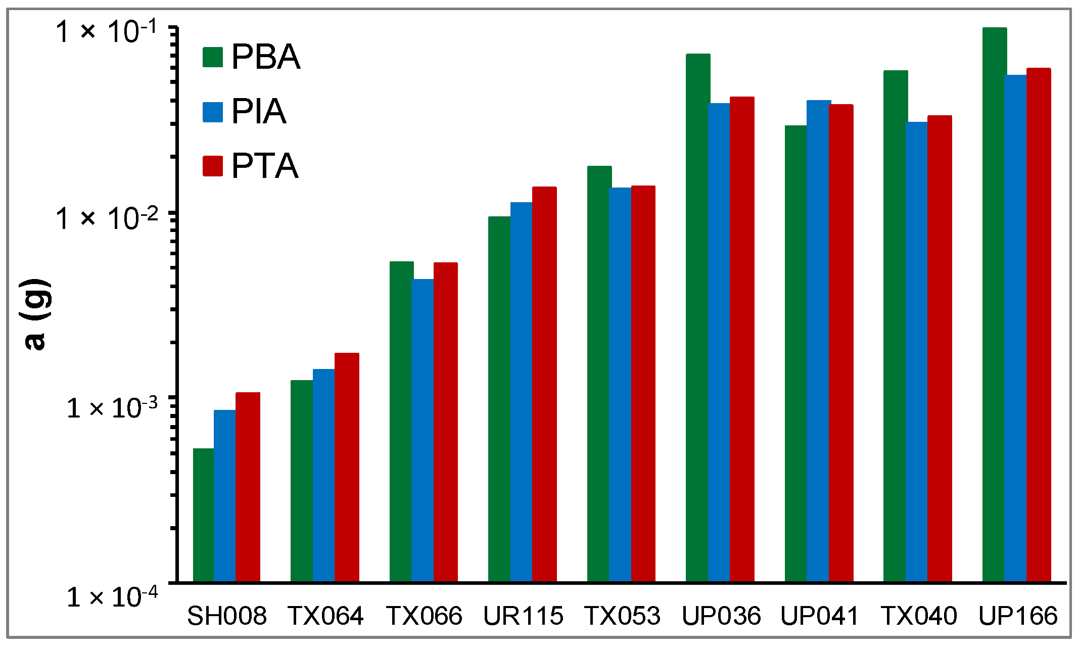
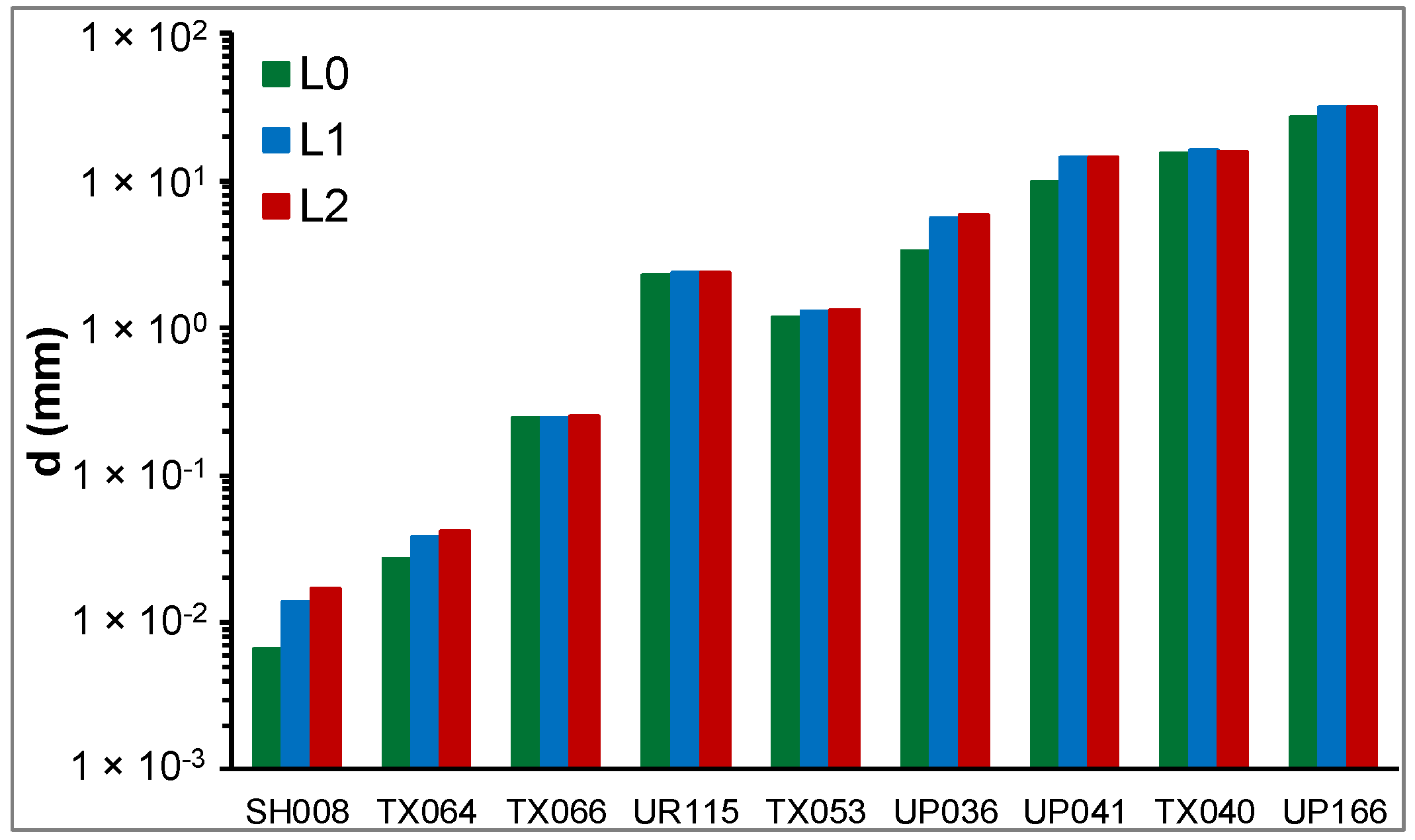
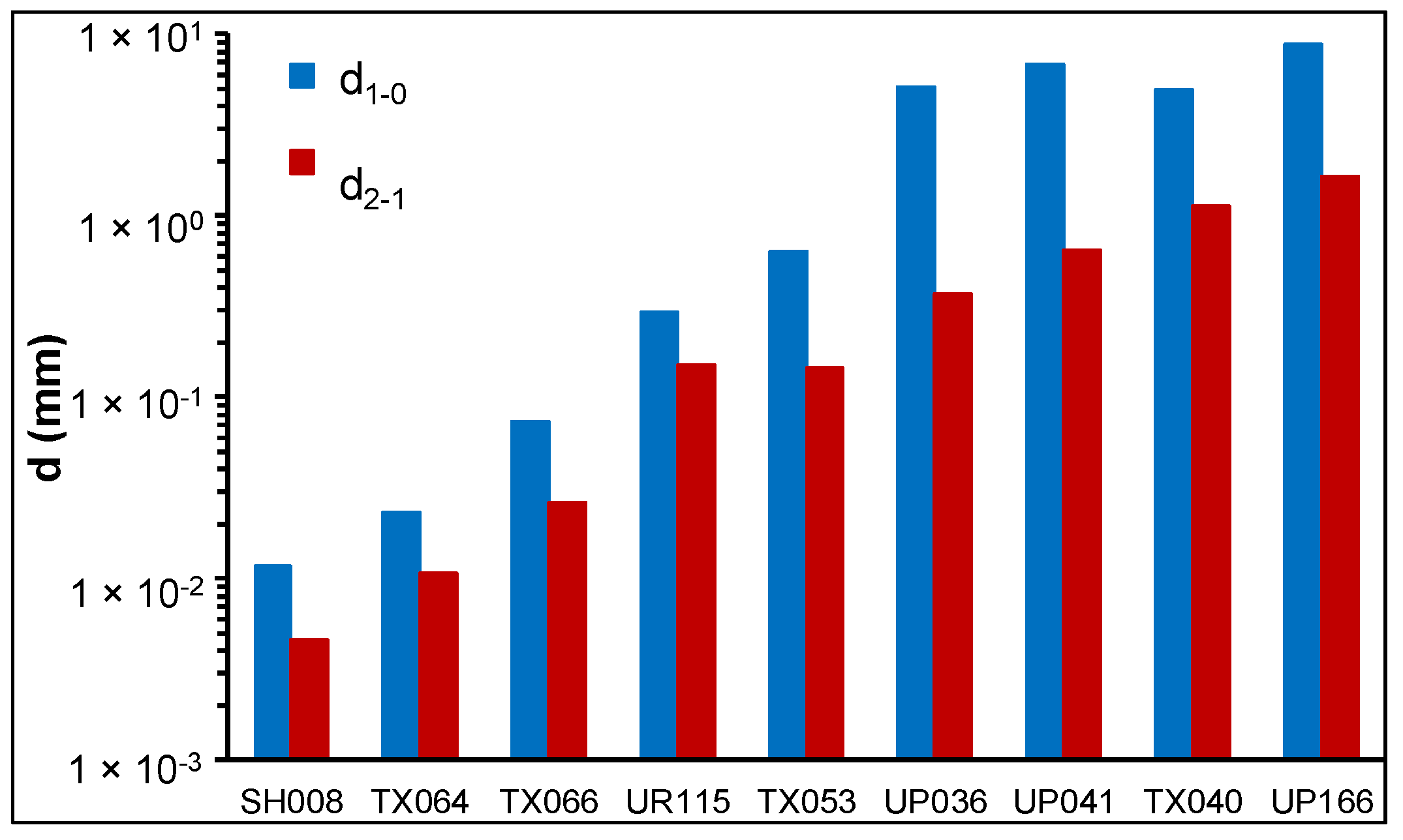
| Event | SH008 | TX064 | TX066 | UR115 | TX053 | UP036 | UP041 | TX040 | UP166 |
|---|---|---|---|---|---|---|---|---|---|
| PBA (g) | 0.0005 | 0.0012 | 0.0054 | 0.0094 | 0.0175 | 0.0706 | 0.0291 | 0.0575 | 0.0975 |
| PIA (g) | 0.0008 | 0.0014 | 0.0043 | 0.0111 | 0.0134 | 0.0379 | 0.0397 | 0.0300 | 0.0539 |
| PTA (g) | 0.0011 | 0.0017 | 0.0053 | 0.0136 | 0.0136 | 0.0411 | 0.0373 | 0.0327 | 0.0589 |
| PBD (mm) | 0.0066 | 0.0271 | 0.2439 | 2.2917 | 1.1813 | 3.3642 | 9.7588 | 15.415 | 27.302 |
| PID (mm) | 0.0138 | 0.0378 | 0.2467 | 2.3663 | 1.3072 | 5.5737 | 14.443 | 16.213 | 31.809 |
| PTD (mm) | 0.0171 | 0.0417 | 0.2524 | 2.3821 | 1.3349 | 5.8568 | 14.367 | 15.765 | 31.956 |
| d1-0 (mm) | 0.0116 | 0.0230 | 0.0728 | 0.2907 | 0.6282 | 5.0766 | 6.7810 | 4.9572 | 8.7882 |
| d2-1 (mm) | 0.0046 | 0.0107 | 0.0261 | 0.1503 | 0.1453 | 0.3685 | 0.6432 | 1.1301 | 1.6426 |
| d1-0 Is01 (mm) | 0.0116 | 0.0224 | 0.0744 | 0.2869 | 0.6686 | 5.0513 | 6.6656 | 5.2281 | 9.2833 |
| d1-0 Is04 (mm) | 0.0142 | 0.0236 | 0.0727 | 0.2847 | 0.6206 | 5.0211 | 6.7040 | 4.7085 | 8.7999 |
| d1-0 Is13 (mm) | 0.0114 | 0.0234 | 0.0730 | 0.2968 | 0.6384 | 5.1327 | 6.8636 | 5.2482 | 8.8119 |
| d1-0 Is16 (mm) | 0.0149 | 0.0251 | 0.0738 | 0.2947 | 0.5880 | 5.1030 | 6.9015 | 4.7466 | 8.3750 |
| d2-1 Is01 (mm) | 0.0045 | 0.0107 | 0.0279 | 0.1439 | 0.1424 | 0.4136 | 0.5993 | 0.9671 | 1.4852 |
| d2-1 Is04 (mm) | 0.0046 | 0.0111 | 0.0292 | 0.1385 | 0.1310 | 0.4408 | 0.5747 | 0.9542 | 1.3457 |
| d2-1 Is13 (mm) | 0.0047 | 0.0113 | 0.0272 | 0.1735 | 0.1680 | 0.3127 | 0.7596 | 1.5602 | 2.1928 |
| d2-1 Is16 (mm) | 0.0049 | 0.0109 | 0.0264 | 0.1631 | 0.1531 | 0.3454 | 0.7973 | 1.5626 | 2.1249 |
| Floor | Self-Weight (kN/m2) | Permanent Load (kN/m2) | Partition Walls (kN/m2) | Variable Load (kN/m2) |
|---|---|---|---|---|
| First | 4.0 | 2.4 | 0.8 | 0.60 |
| Second | 4.0 | 4.9 | 0.8 | 0.60 |
| Third | 4.0 | 2.7 | 0.0 | 0.00 |
| Mode | Frequency (Hz) | Period (s) |
|---|---|---|
| 1 | 0.391 | 2.554 |
| 2 | 0.392 | 2.552 |
| 3 | 0.493 | 2.026 |
| 4 | 2.952 | 0.339 |
| 5 | 3.394 | 0.295 |
| 6 | 3.447 | 0.290 |
Publisher’s Note: MDPI stays neutral with regard to jurisdictional claims in published maps and institutional affiliations. |
© 2022 by the authors. Licensee MDPI, Basel, Switzerland. This article is an open access article distributed under the terms and conditions of the Creative Commons Attribution (CC BY) license (https://creativecommons.org/licenses/by/4.0/).
Share and Cite
Salvatori, A.; Bongiovanni, G.; Clemente, P.; Ormando, C.; Saitta, F.; Scafati, F. Observed Seismic Behavior of a HDRB and SD Isolation System under Far Fault Earthquakes. Infrastructures 2022, 7, 13. https://doi.org/10.3390/infrastructures7020013
Salvatori A, Bongiovanni G, Clemente P, Ormando C, Saitta F, Scafati F. Observed Seismic Behavior of a HDRB and SD Isolation System under Far Fault Earthquakes. Infrastructures. 2022; 7(2):13. https://doi.org/10.3390/infrastructures7020013
Chicago/Turabian StyleSalvatori, Antonello, Giovanni Bongiovanni, Paolo Clemente, Chiara Ormando, Fernando Saitta, and Federico Scafati. 2022. "Observed Seismic Behavior of a HDRB and SD Isolation System under Far Fault Earthquakes" Infrastructures 7, no. 2: 13. https://doi.org/10.3390/infrastructures7020013