1. Introduction
Designing new or existing transportation facilities requires accurate surface terrain information [
1]. Conventional survey methods for acquiring accurate terrain surfaces include Real Time Kinematic Global Positioning System (RTK-GPS), Electronic Distance Measurement (Total Station), and photogrammetry. Generally, RTK-GPS and Total Station procedures are time-consuming and costly due to the necessity of workers and equipment needing to physically move across the terrain of an area to achieve satisfactory coverage. Certain operational constraints such as dense vegetation cover must also be considered, and in the case of conventional survey on existing road design projects, vehicular traffic is a further safety consideration. While large-area terrain information can be collected through these methods, the time and effort needed is significant.
Photogrammetry circumvents some of the limitations of RTK-GPS and Total Station survey but introduces other issues. Imagery used for photogrammetric data must typically be gathered in highly specific conditions, usually when foliage is in a bare, leaf-off state but before the ground is covered by snow and ice [
1]. Photogrammetry also requires a particular sun angle with no cloud cover present. Once photogrammetric imagery is collected, processing the data and determining elevation is often time-consuming.
Lidar data is an alternative to these methods and may be used for road design if their accuracy is within an acceptable range. UAV photogrammetric capture data is another option, especially for smaller areas. Even though UAV photogrammetric capture is based on photogrammetry, it is a much lower cost alternative relative to aerial photography and can be convenient for smaller projects. In fact, UAV photogrammetry may produce better results, when properly controlled with appropriate ground control, than traditional manned-aircraft photogrammetry because it produces positions from images that are so much closer to the ground, so resolution can be much better, especially if high-end UAV sensors are used. The speed an airplane has to maintain to keep it in the air makes it impossible to get clear images from 400′ off the ground—A typical ceiling for small UAVs - so pixels, even of high-end wide-format cameras costing millions of dollars, refer to larger areas of land than in many small UAV models. Typical manned flight imagery provides a pixel resolution of 7.6 cm for highways; the UAV pixel resolution in this study was 1.6 cm.
To assess the suitability of these alternative methods for road design applications, it is necessary to understand accuracy standards recommended for such work. According to the Idaho Transportation Department’s (ITD) 2018 Standard Specifications for Highway Construction, original ground confidence point vertical tolerance values are as shown in
Table 1 [
2]:
An additional measure to check the accuracy of the collected Lidar data is to compare the Root Mean Square Error (RMSE) for the difference between the remote source data and the conventional survey data with the standard accuracy limit stipulated by the Idaho Lidar Consortium (ILC). According to ILC, any RMSE less than 12.5 cm is within their accuracy standard [
3]. ILC defines three types of vertical accuracy: Fundamental, Supplemental, and Consolidated. The accuracy threshold specified above is for Fundamental Vertical Accuracy (FVA), which is applicable for open terrain. In other words, FVA is applicable when we can assume that the sensor is able to detect the ground surface.
By supplementing these data with survey control methods, a high degree of accuracy can be achieved. Lidar (light detection and ranging) is an active remote sensing technique that uses laser light to measure distance by illuminating an object and measuring the reflected light with a sensor. Common acquisition methods include mounting a lidar device on an aircraft or ground-based vehicle and moving while the device continuously collects point data. The result is a “point cloud” dataset of lidar point locations, from which elevation models can be created. Compared to the previously described conventional survey methods, lidar is generally considered to offer safer data collection, cost effectiveness, and a high level of detail [
4].
Another remote sensing technique is the use of an unmanned aerial vehicle (UAV) to acquire photogrammetric capture data through the collection of a large volume of photographs. This method utilizes a digital structure from motion process with scale invariant feature transform tools. Essentially, this uses the parallax differences between photographs to generate a three-dimensional model of its target. A digital surface terrain model can be generated using this output, as well as a point cloud file or files resembling a lidar point cloud dataset. Although this method has some of the same issues as “traditional” photogrammetry, it is generally considered a less-expensive alternative to both conventional survey and lidar.
The accuracy of lidar data has been compared to conventional survey points in other research. For example, Pourali et al. utilize this general technique to determine vertical accuracy for a test lidar dataset, noting its suitability for purposes requiring an accuracy of up to 0.5 m for a large area of aerial lidar in Victoria, Australia [
5]. Hodgson and Bresnahan used a similar approach to test aerial lidar accuracy as part of a large-scale mapping effort for Richland County, South Carolina [
6]. Lidar accuracy depends on the entire workflow starting from data acquisition through generating the final terrain model. Researchers have noted that high quality digital terrain models (DTMs) can be generated with suitable processing techniques, which take into account a variety of factors including the multiple returns lidar typically produces [
7]. For example, classifying lidar data allows for differentiating between the ground, foliage, buildings, and water surface in the point cloud. Besides roadway design, lidar is routinely used in a variety of applications including forest inventory and assessment [
8,
9], hydrologic channeling [
10], and carbon sequestration [
11].
Lidar used for roadway design is usually collected expressly for this purpose, and studies [
5,
6] have shown a root mean square error (RMSE) of 0.18–0.50 m for vertical accuracy. One of the earlier studies has reported RMSEs between 0.06–0.10 m over a road right-of-way [
12]. But this low level of RMSE was achieved after removing systematic biases that ranged from about 20 to −10 cm. In the years since these studies, improvement in lidar accuracy is reflected in standards such as the latest USGS Lidar Base Specification. This publication lists a relative vertical accuracy of less than or equal to 0.06 m for smooth surface repeatability and 0.08 m for swath overlap difference [
13]. The accuracy of lidar-derived digital elevation model (DEM) rasters has been researched over a variety of vegetation and terrain types [
14]. One study indicates that increasing terrain slope leads to lower lidar canopy height estimates because slope has effect on DEM accuracy [
15]. As part of this study, the effects of both slope and terrain type on lidar vertical accuracy will be examined.
The Australian study cited above [
5] has reported vertical accuracy from aerial lidar of 50 cm. Their definition of vertical accuracy was a 95% confidence interval assuming a normal distribution of RMSEs. In other words, the vertical accuracy reported was 1.95 times the mean RMSE. Using this definition, the vertical accuracy for our study, as will be seen later, will calculate to 17.7 cm, which is much lower than the 50 cm reported in the Australian study. This difference is remarkable since the procedure to estimate RMSE in the Australian study was very elaborate compared to the method used in our study. All lidar points within 1 m of a Ground Control Point (GCP) were identified in the Australian study. The points were ranked in terms of the distance from the GCP. RMSEs for the set of points closest to the GCPs were computed, followed by the points second closest to the GCP, and so on. The RMSEs were then averaged. This elaborate procedure was adopted supposedly to prevent interpolation errors which are thought to be introduced when deriving elevations from a DEM generated from the lidar point elevations. Our study used such a DEM generated by ArcGIS. Yet the accuracy obtained in this study was higher than the one reported by Pourali et al. [
5].
Another study that has examined accuracy of airborne lidar as reported earlier is by Hodgson and Bresnahan [
6]. In Hodgson and Bresnahan study, elevations of selected lidar points were measured using conventional survey methods and compared with the lidar-determined elevations. This was done to control for errors that could potentially be introduced when interpolating from a DEM. This is in contrast to what was done in our study, where ground points were first established and their elevations measured. These elevations were then compared with the elevations estimated for these points using a DEM that was created from lidar points. The RMSE obtained by Hodgson and Bresnahan for pavement surface was 18.9 cm, which is much higher than the value reported in our research for pavement surface as will be shown later in this paper. In fact, the overall RMSEs obtained in our research are lower than 18.9 cm. This difference in findings in the two studies cannot be explained easily. Perhaps this is due to the improvement in the technologies of data collection and processing between the time the data used by Hodgson and Bresnahan were collected (October 2000) and the time when the data used in our study was collected (April–October 2016).
The civil engineering application addressed by this study is highway design. One study that measured elevations along a road corridor, as mentioned previously, was performed by Shrestha et al. [
12]. Shrestha et al. state that the RMSE in their study “was approximately 6 to 10 cm over the entire right-of-way”. This is a remarkable achievement, which is especially noteworthy because the data for their study was collected in November of 1997. None of the other more recent studies have reported accuracy levels of this order. It should be noted, however, that Shrestha et al. state that systematic biases that ranged from 20 cm to −10 cm were removed from their data during calibration. The aerial lidar data used in our study was provided by Aero Graphics and we have no knowledge of their data processing efforts prior to submitting the data to ITD.
Review of literature on this topic has revealed that use of remote sources of data in highway design is sparse. And the studies that have explored this topic have reported widely varying accuracy levels. The accuracy levels reported have also been found not to be commensurate with the complexity of analytic methods used in the processing of the data. So, the main motivation of our study was to conduct and present a simple side-by-side comparison of remote data collection systems commonly available to highway design staff in state departments of transportation and engineering firms that provide design services to highway agencies. Analytical methods and software used in this study are similar to those readily available to agency staff. We hope that the findings from our study will encourage highway agencies to make more use of this readily available technology in some aspects of highway design.
Study Objectives
The following objectives were considered for this study:
Compare the vertical accuracy of the three test case datasets to traditional survey elevation ground points,
statistically determine whether the elevation differences between the test datasets are potentially acceptable for use in roadway design, and
perform a cost analysis of the different data collection methods.
3. Results
3.1. Elevation Difference—Overall
Table 2 shows the difference in elevations obtained from the conventional survey and each remote method DEM for all survey point locations using ArcMap. The conventional survey elevations were used as the “true” elevations.
The difference in elevation represented in
Table 2 is the conventional survey elevation minus the elevation obtained from one of the three remote sources of data. Elevation differences for all locations irrespective of the ground slope or surface type were used. The mean difference was found to be negative for all three remote data sources, indicating that on average the remote data sources overestimated the ground elevation. The table shows that the aerial lidar elevations are closer to the surveyed elevations than those from the other two sources. The RMSE for mobile-terrestrial lidar was the highest in this analysis, with similar results for mean difference and standard deviation. The relative standard deviation values show that the mean differences had large variations. The relative standard deviation measure is comparable to the coefficient of variation statistic. The coefficient of variation statistic can be misleading when the mean of a random variable is a negative quantity, which is the case with the mean difference in
Table 2. Hence, the absolute mean difference (MD) was computed and used to calculate the relative standard deviation.
3.2. Elevation Difference—By Study Section
Table 3 shows the results for the three road sections in which the verification survey data was collected. In all cases, the RMSE and standard deviation were high in
Section 1. This was also true for mean difference except for the aerial lidar elevation differences. As in the aggregate case shown in
Table 2, the precision of the measurements was higher in the case of aerial lidar relative to the other two sources.
Section 2 for both mobile-terrestrial and UAV data had the greatest variability as indicated by the relative standard deviation measure.
3.3. Elevation Difference—By Surface Type
Table 4 presents the elevation differences for road- and non-road-surfaces. The RMSE for the road-surface points is much lower than that for the non-road-surface points. The RMSE for road-surface for all remote source data is quite acceptable within the standard accuracy limit stipulated by the Idaho Lidar Consortium (ILC). For points on the road-surface, mobile-terrestrial lidar gave the most accurate result among the three sources of data, while the aerial lidar had the highest RMSE (5.4 cm). The mean differences and standard deviations were also low for all remote data sources. It can be concluded that on road-surface areas, all these data types provide acceptable results.
However, similar results were not observed for non-road-surface areas. The RMSE was high for all the remote data sources, with RMSEs higher than the 12.5 cm ILC standard for mobile-terrestrial and UAV sources. In terms of the ITD Highway Construction Specifications data for all remote sources met the verrtical tolerance values for natural ground. Aerial lidar achieved the closest result in terms of RMSE, mean difference, and standard deviation. This indicates that vertical accuracy of both the lidar and UAV photogrammetric data is significantly affected by non-road-surface returns for all of the alternatives. To summarize, it can be concluded that lidar and UAV photogrammetric data collected using survey control can achieve high accuracy for areas over a road surface with diminished accuracy for non-road surfaces.
The variability of mobile-terrestrial and UAV data appear to be high relative to aerial lidar data as measured by the relative SD statistic. This is because the relative SD measure takes larger values when the mean of the related random variable is smaller and is closer to zero.
3.4. Elevation Difference—By Terrain Slope
Table 5 shows results by slope of the ground using the previously described slope classification. From the table it can be concluded that the RMSE for aerial lidar was noticeably lower for moderate and steep slope areas when compared to either the mobile-terrestrial lidar or the UAV photogrammetric data. There were 922 survey points across the three road sections of the study area, and of these only 36 points were identified as level. More than half of the points were considered moderate, a total of 494 points, and 392 points were considered steep. The RMSE for all remote data types was lowest at points considered to be on level terrain. The RMSE for aerial lidar differences at points considered level was 4.91 cm. The aerial lidar data had its highest RMSE in steep areas, at 11.00 cm, which is below the ILC standard of 12.5 cm. This, along with its RMSE of 7.48 cm for moderate areas, explains why the overall RMSE, all points considered, was lowest for the aerial lidar.
The variability in the measurements was also lower for aerial lidar data compared to the other two sources. It should be noted that the relative standard deviation of 225% for flat surface data collected by mobile-terrestrial lidar is misleading and is due to the low mean difference value for this case.
The RMSE for the mobile-terrestrial lidar was higher than aerial lidar for terrains with moderate or steep slopes. A total of 920 conventional survey points was available for comparison of the mobile-terrestrial lidar. Of these 920 points, only 39 points were on ground considered level. The highest number of points were considered moderate, a total of 458. The remaining 423 points were considered steep. The mobile-terrestrial RMSE was 4.36 cm for level terrain, which was low compared to that for aerial lidar. The highest RMSE for mobile-terrestrial lidar was obtained in steep areas with an RMSE value of 24.57 cm, while in moderate areas the RMSE was 10.99 cm. The overall RMSE was high, due to the higher RMSE in the steep areas. Similar patterns are apparent in the mobile-terrestrial mean difference and standard deviation for each terrain type. All values were high for steep regions and low for level regions, following a pattern similar to the aerial lidar.
The UAV photogrammetric data had a total of 918 usable survey points. Only 45 points were determined to be on level terrain. Among the three types of remote data, the UAV-based DEM had the highest number of survey points considered level and the RMSE was the lowest among all of them, with an RMSE for level terrain of 3.95 cm. RMSE of the points considered to be on moderate terrain was 9.92 cm. This RMSE was lower than that for the mobile-terrestrial lidar but higher than for aerial lidar, with 436 survey points considered on moderate terrain. A similar number of points were obtained for steep areas, 437 in total. The RMSE for steep areas was 18.94 cm, which was the highest among the three types of terrain areas. Notably, the UAV data for steep areas was closer in accuracy than the mobile-terrestrial lidar. The mean difference and standard deviation for the UAV data appear to generally follow the same patterns as for the aerial lidar and mobile-terrestrial lidar. It is noted that the mean difference for all remote sources and slope types was within the vertical tolerance limit specified by ITD for natural ground. And except for areas with a steep slope for mobile-terrestrial and UAV data, all mean differences were with the vertical tolerance limit for graded surface.
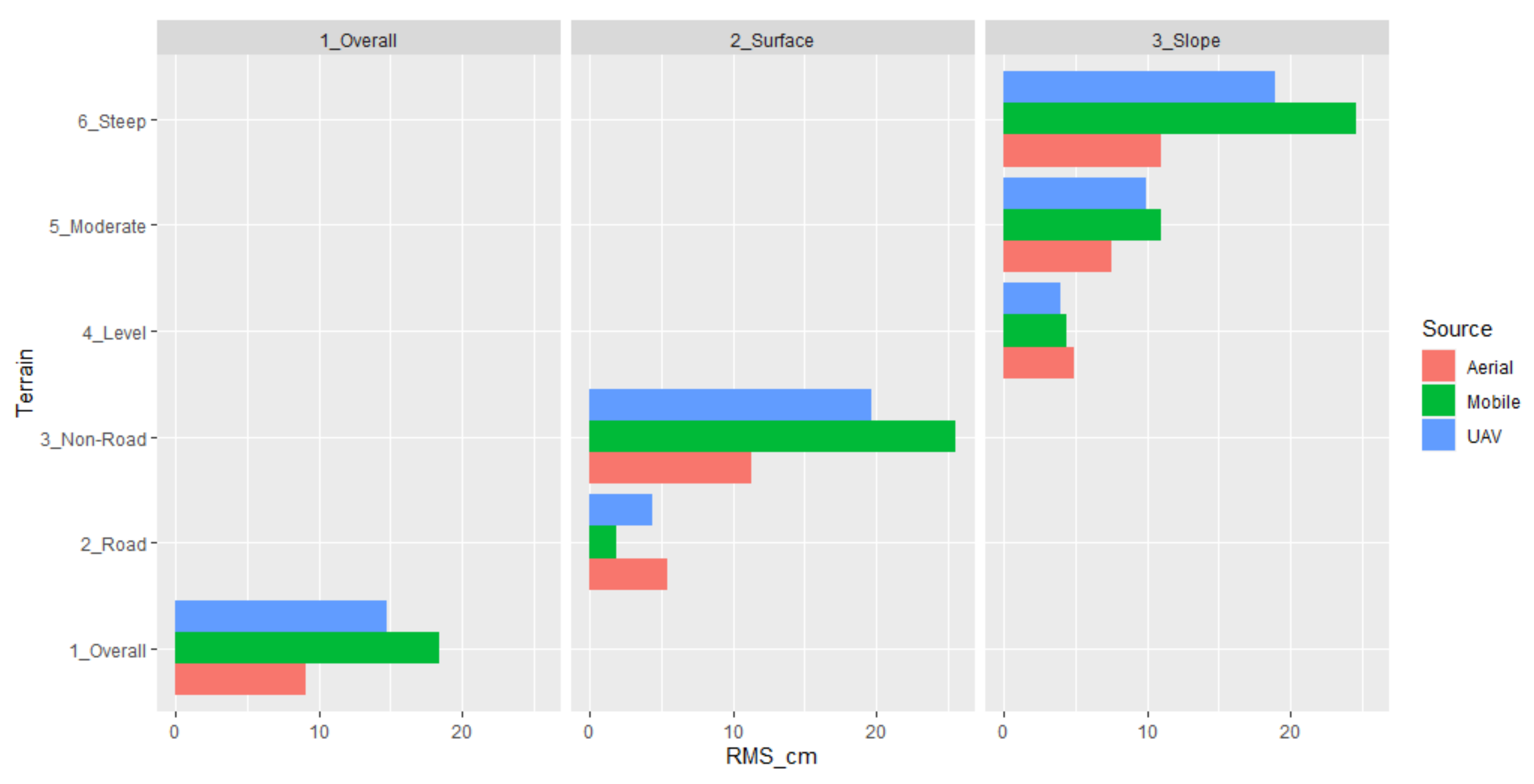
3.5. Summary of Elevation Differences
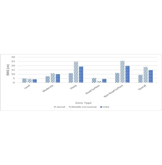
In
Figure 4, the RMSEs for the aerial lidar, mobile-terrestrial lidar and UAV photogrammetric data are shown for the different areas including the overall RMSE for these data sources. The figure illustrates that the aerial lidar elevations were generally the closest to the conventional survey elevations, although the RMSE for level areas was higher than the other two data types. However, this difference is relatively minimal. The UAV data had the second-closest elevational accuracy compared to the conventional survey, and mobile-terrestrial lidar had the least accurate RMSE, in large part due to steep areas and those away from the road surface. As noted previously, the verification survey locations were intentionally chosen as areas where the mobile-terrestrial lidar collection was likely to have difficulty with terrain away from the roadway.
3.6. Statistical Analysis Results
The two types of statistical analyses discussed earlier were performed on selected data sets presented in
Table 2,
Table 3,
Table 4,
Table 5. The first type is the estimation of confidence intervals around the mean difference for the various data sets shown in the tables. The second type of anlysis is to estimate confidence intervals around the calculated RMSE
3.6.1. Confidence Interval around Mean Difference
To find a confidence interval around the mean elevation difference the first step needed is to determine whether the differences are normally distributed. To this end, histograms were constructed for all differences described in
Table 2,
Table 3,
Table 4,
Table 5.
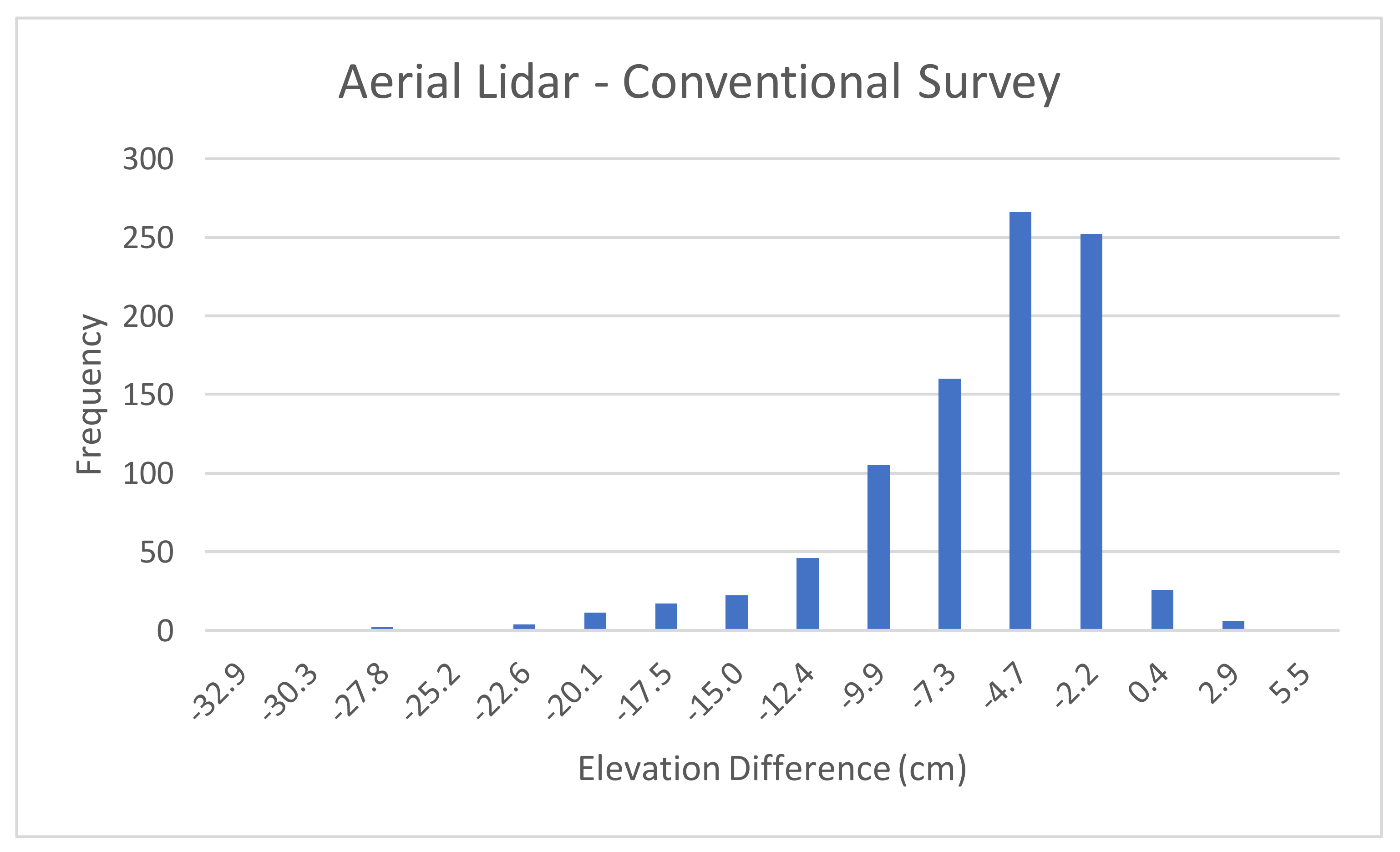
Figure 5 depicts the histogram for the difference between elevations computed using aerial lidar and conventional survey data. The mean for the differences, as noted in
Table 2, is −7.48 cm. The figure shows that the histogram is not centered around this mean; the diagram is skewed to the left. There were also some outliers with high negative elevation difference
Figure 6 depicts a similar histogram of differences between the mobile-lidar based elevations and the elevations estimated using conventional survey. The mean of the differences for this case is −9.04. The histogram does not imply that the distribution of differences is centered around this mean value. The figure also shows that there some outliers in this data set.
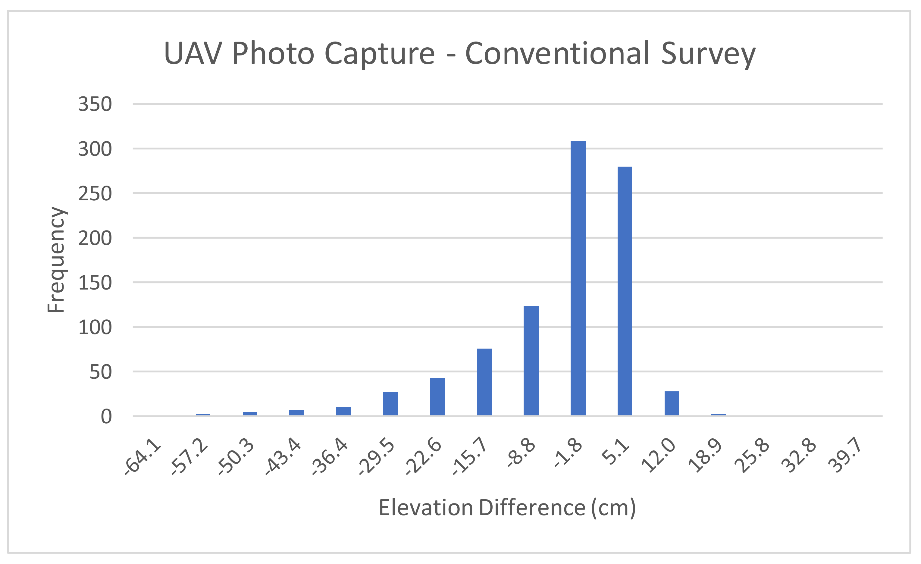
Figure 7 depicts the histogram of differences between the UAV photogrammetric capture data based elevations and the elevations estimated using conventional survey. The mean of the differences for this case, as shown in
Table 2, is −7.79 cm. The histogram shows that the elevation differences are not normally distributed around this mean. The figure also shows that there are some outliers in the data.
Since confidence intervals based on mulitples of the standard deviation around the mean cannot be used for any of the three cases above Chebyshev’s Inequality was used for this purpose. Using Equation (1) the confidence intervals for the Mean Difference shown in
Table 2 for the three remote sources with
h = 2 are: aerial: (−17.78, 2.82), mobile-terrestrial: (−43.4, 25.32), and UAV photogrammetric capture data: (−32.93, 17.39). The probability that the mean difference for each of the three remote sources will be in these intervals is at least 75%. The intervals are wide and hence are not precise. But each of the intervals contains zero, a mean difference value that will be obtained when the measured elevations are, on the average, exactly equal to the assumed true values.
The Chebyshev’s Inequality analysis was only done on the aggregate elevation data shown in
Table 2. This analysis can be extended to all mean differences for the disaggregated data shown in
Table 3,
Table 4,
Table 5. The confidence intervals for some of these cases will be smaller because of lower values of mean difference as well as the associated standard deviation.
3.6.2. Confidence Interval around RMSE
Confidence intervals were computed using the formulation shown in Equation (2) for selected RMSE values shown in
Table 2,
Table 3,
Table 4,
Table 5. As mentioned in
Section 2.4 above, only RMSE values that are slightly over the limit of 12.5 cm will be tested. The RMSE value which fits this criterion is the one for UAV in
Table 2.
Using Equation (2),
for the overall UAV data was estimated to be 0.34. The RMSEs for this case as shown in
Table 2 is 14.77 cm. Using
h = 3 in the formula for Chebyshev’s Inequality (Equation (1)), the 89% confidence intervals for the RMSE is (13.74, 15.81). Since even the lower limit of this interval exceeds the ILC threshold of 12.5 cm, the overall UAV data does not meet the ILC standard. The confidence interval for the overall mobile-terrestrial RMSE was not computed as the RMSE for this source is even higher than the one for UAV. The lower limit for the 89% confidence limit for the mobile-terrestrial lidar RMSE is also expected to exceed the ILC threshold. Hence, the accuracy of the mobile-terrestrial lidar data, when considered as a whole, does not meet the ILC standard.
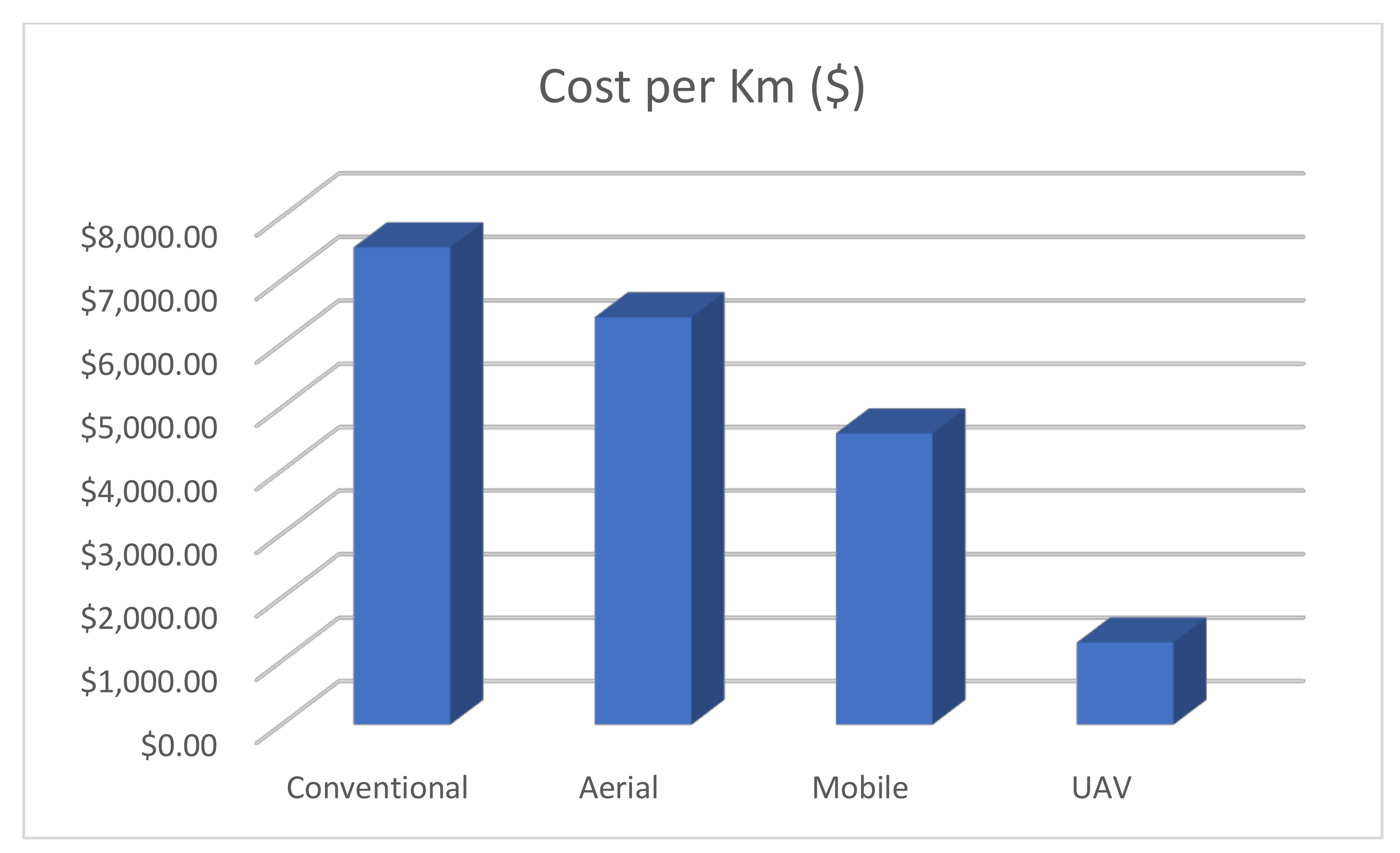
3.7. Cost Comparison
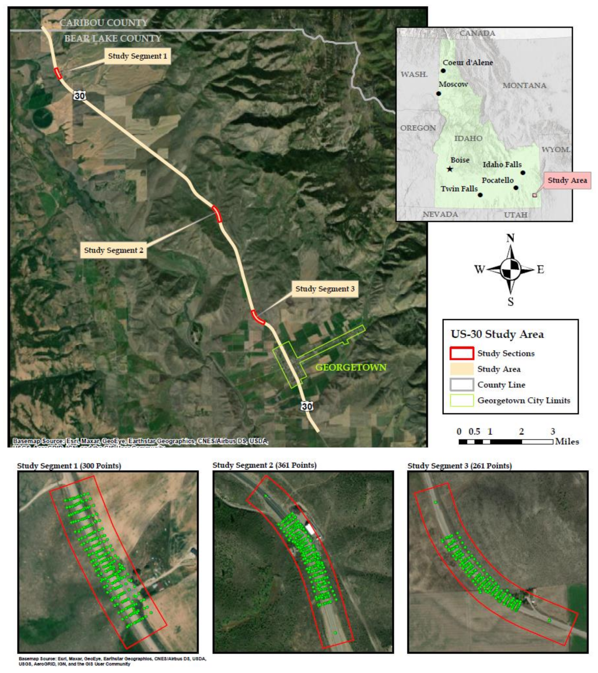
For the cost comparsion, the twelve miles of US-30 between mileposts 413 and 425 where the mobile-terrestrial lidar was collected in Bear Lake County are considered.
Table 6 lists the costs of collecting and processing each data type for a roadway project of this magnitude:
The conventional survey cost refers to the use of a Total Station to record optical data observations. This methodology was used in the conventional survey verification cross-sections, used as the basis for all accuracy comparisons in this study. ITD paid Dioptra Geomatics
$6877.68 for the approximate 915 m of cross-sections of highway surveyed for project A019(382) to produce the three verification cross-section areas. The above cost was derived as follows:
The planning-grade aerial lidar used in this study is part of a districtwide collection effort, including 1152 linear km of roadway. Economies of scale are important to note in determining the cost of such an extensive project. The total cost of the project, including ground survey control by AeroGraphics’ survey crew, as well as the collection of aerial imagery by Aero-Graphics, Inc., orthorectified imagery, DEM raster surfaces, and other data processing, was $486,000, from which the 19.31 km and per km figures were derived.
However, if a consultant collected aerial lidar on a more limited basis at design-grade (as the mobile-terrestrial lidar was), rather than districtwide at planning-grade, the cost would likely be significantly more. This may in large part be due to the necessity of mobilizing the collection aircraft. To approximate this cost, a comparable aerial lidar collection effort such as that for ITD project keys 14,002 and 13106, flown in 2014, could be used for comparison. The invoiced amount of the combined lidar collection for these projects was $123,992.58.
It should be noted that the comparison here is not perfectly analogous to the US-30 project area, as it is for a different part of the highway system, multiple stretches of highway, and includes numerous side roads, which may make for a more complex flight pattern. However, the total highway distance with these two roads is similar to the US-30 study area and should make for a reasonable comparison with the US-30 study area data costs.
The total invoice for the mobile-terrestrial lidar collected by R.E.Y. Engineers, including control, supplemental survey data, and conventional verification data by Dioptra Geomatics, was
$88,646.40. This collection spanned 19.31 km (12 miles) between MP 413-425 on US-30. Finally, because the UAV photogrammetric data was collected and processed in-house by ITD, the cost in the table is an approximate estimate of the cost as provided by consultants.
Figure 8 depicts the cost comparison pictorially.
4. Discussion
Table 7 below presents how the data shown in
Table 2,
Table 3,
Table 4,
Table 5 compare with the ITD specification for vertical tolerance and the ILC vertical accuracy standard. An “yes” in a cell for any row with “RMSE” in the first column indicates that the source data for the cell satisfies the ILC standard. The word in a cell for any row with “Mean Difference” in the first column denotes the surface type for which the vertical tolerance shown in
Table 1 is met. For example, if the word in a cell is “Graded” for any “Mean Difference” row, it means that the vertical tolerance for the remote data source satisfies ITD’s highway construction specification for machine graded and compacted surface.
In terms of the RMSE standard stipulated by ILC, aerial lidar data was found to be satisfactory in all cases: overall, by study sections, by surface type, and by terrain slope. Mobile-terrestrial and UAV photogrammetric capture data on the other hand did not meet this specification when the data for the entire study area is considered. When examined in a more disaggregated fashion they met the standard in some cases. For example, mobile-terrestrial data met the ILC standard in
Section 2, on road surface, and on level and moderate slopes. Likewise, UAV photogrammetric capture data met the ILC standard on road surface and on level and moderate slopes.
In terms of ITD’s vertical tolerance limits for highway construction, all three remote data sources were within the tolerance limit for machine graded and compacted surface when viewed at an aggregate level covering the entire study area. This is a significant finding. This implies that terrain models created using remotely collected data can be used for new road designs as well as reconstruction and rehabilitation of existing roads.
At more disaggregated levels, when ground surface type and slope of the terrain are considered, the accuracy of each data type degraded at higher steepness and off-pavement. Spaete et al. have noted that vegetation and slope areas have a statistically significant impact on the accuracy of lidar-derived DEMs [
21]. Our study has indicated that the aerial lidar provided the most accurate terrain information in these areas. Considering the vantage point of the aerial lidar with its capability of multiple returns, this makes sense. The mobile-terrestrial lidar is understandably limited by its ground vantage point, especially in areas with steep slopes.
The three conventional verfication areas were deliberately selected to be areas likely difficult for the mobile-terrestrial to achieve accuracy away from the pavement. The UAV photogrammetric capture method, while having an aerial vantage point, is limited by being based on photographic images. This means foliage is likely to have a major impact on its accuracy. Another possible consideration is the processing method each remote. las dataset received. The aerial lidar received some manual processing, while the mobile-terrestrial and UAV data both relied on an automated ground-classifying process in ArcMap. Manual processing of the mobile-terrestrial lidar and UAV photogrammetric data may improve the accuracy of these data types in off-road and steeper areas.
It is also important to point out that the difference in implications from the two set of standards, the ILC standards for RMSE and the vertical tolerance limits from ITD’s Highway Construction Specifications. According to the latter the vertical accuracy from all three remote sources satisfy the requirements for natural ground for all types of surfaces and for all degrees of slopes. That is not the case when using the ILC standard for RMSE. If the ILC standard is used, then only aerial lidar will be suitable for all types of surfaces and all degrees of slope. Mobile-terrestrial and UAV photogrammetric capture data do not satisfy the ILC standard for RMSE for non-road surfaces and grounds with a steep slope.
The vertical accuracy levels we were able to achieve in our research were not the same as those claimed by the vendors who collected the aerial lidar and mobile-terrestrial lidar data. As mentioned in
Section 2.2 above the aerial lidar data vendor have claimed an RMSE of 3.14 cm for open and non-vegetated areas. The lowest RMSE we were able to achieve with aerial lidar data was 4.91 cm for level areas as shown in
Table 5. Similarly, the mobile-terrestrial vendor claims an RMSE value of 0.732 cm for pavement plus edge of pavement and 4.3 cm for “ground” points; these are points not on pavement or edge of pavement. These RMSE of error values are lower than what we were able to achieve. As can be seen in
Table 4, 1.9 cm was the lowest RMSE value we obtained with mobile-terrestrial data; this was for points on a road surface. Further research is needed to explain these differences in accuracy levels. However, it can be stated here that highway agencies are advised to conduct random quality assessment of data received from outside vendors.
Regarding the UAV data, the RMSEs of error between control point elevations and point cloud derived elevations were 17.1 cm, 1.9 cm, and 15.8 cm respectively for the three study sections, as stated in
Section 2.2 earlier. RMSE values obtained in our study for the three sections were 17.4 cm, 13.6 cm, and 12.9 cm, as shown in
Table 3. Except for
Section 2 the two sets of RMSE values are comparable. It is to be noted that the UAV data was collected in-house by ITD unlike the two other remote sources of data.
In closing, a stepwise recommendation to highway agencies about using vendor-supplied, remote source data for highway design is provided below:
Require a detailed explanation of vertical accuracies from vendors. The vendor report should include details about the software used in the processing of the point cloud data.
Divide your project area into at least thirty, approximately equal regions.
Establish a verification point in each of the regions and measure the elevation of the point using a conventional survey method, such as a Total Station or RTK-GPS.
Estimate the elevation of each of the points using a DEM based on the remote source data obtained from the vendor.
Compute the RMSE and the average difference in elevation between the two sets of elevations.
If the values obtained in Step 5 above meet applicable standards for your jurisdiction, the DEM derived from the remote source data may be used for highway design.
If the test in Step 6 is not successful, do not accept the vendor supplied remote source data.


