Deep Learning Approaches for Long-Term Global Horizontal Irradiance Forecasting for Microgrids Planning

Abstract

Providing sustainable energy to rural communities is considered in Sustainable Development Goal 7. Off-grid renewable energy systems arise as an affordable solution due to their portability and the availability of renewable sources for rural communities. In this work, to deal with the uncertainties of solar resources, we employ two deep learning models (feed forward and recurrent neural networks) to predict renewable sources in a long-term horizon. To this aim, the approach presented takes into account the necessity of a high enough resolution in the forecasting output. As a case study, we employ open source data for a location in Michoacan, Mexico as well as open source programming frameworks to ensure the replicability of the numerical experiments. The results show that our prediction model performs excellently with respect to the baseline methods (ARIMA, exponential smoothing, and seasonal naive) in terms of the evaluation metrics MASE (18.5% of reduction with respect to seasonal naive), RMSE (24.7%), WAPE (13.1%), MAE (12.9%), and APB (8.9%).

1. Introduction

Although the COVID-19 pandemic has slowed down the global energy demand growth, an increase between 4% and 9% is estimated between the years 2019 and 2030 [1]. Furthermore, there are around 840 million people without electricity access [2], and the vast majority (85%) come from rural areas [1,2]. In this context, hybrid renewable energy systems (HRES) constitute an affordable solution to electrify rural areas, given the technologies’ portability and their usefulness to reduce greenhouse gases emissions [3,4].

Several configurations of hybrid renewable energy systems (HRES) are analyzed in the literature, combining different technologies, the most common being solar photovoltaic arrays (PV) and wind turbines (WT) along with storage batteries [5,6]. For instance, Ref. [7] presents a stand-alone system based on solar PV generators hybridized with internal combustion engines and micro gas turbines. This work is focused on the analyses for cost of energy (COE), waste heat, duty factor, and life cycle emissions (LCE). Likewise, in [8] the techno-economic and performance analysis of a microgrid integrated with solar, wind, diesel and storage technologies is carried out. The mathematical modeling of these technologies has been widely studied [9,10]. The modeling aspects are important considerations to be accounted for in optimization procedures. A comprehensive review of state-of-the-art problem formulations related with solar and wind energy supplies along with machine and deep learning techniques applied in this field is presented in [11].

Classical and modern optimization methodologies have been employed for the optimal sizing of HRES [5]. These techniques are referred in the literature as three different methods: classical, meta heuristic techniques, and computer software [12]. Classical methods involve the use of linear programming (LP) [13] problems, mixed integer linear programming (MILP) problems [14], analytical [15], and numerical [16] methods. Meta-heuristics involve the use of a single [17] or an hybrid [18] algorithm. Finally, some of the most used software are HOMER [19] and ViPOR [20]. A complete review of the latter category is presented in [19]. The optimal sizing of HRES raises the importance of counting on accurate and long-term solar radiation forecasting.

The vast majority of solar forecasting techniques are focused on the short and mid terms [21]. For instances, a probabilistic approach is presented to calculate the clearness index in [22]. Ref. [23] presents a hybrid model which entails variational mode decomposition (VMD) and two convolutional networks (CN) together with random forests (RF) or long short-term memory cells (LSTM) to predict 15 min ahead or up to 24 h.

Deep learning (which is entailed in machine learning) is about obtaining structural descriptions that contain information from raw data [24]. Four fundamental architectures of deep learning are feed forward neural networks (FFNN), convolutional neural networks (CNN), recurrent neural networks (RNN), and recursive neural networks. Automatic feature extraction is one of the main advantages that deep learning exhibits over traditional machine learning (ML) methods. Furthermore, the latter ones are based on linear combinations of fixed nonlinear basis functions, whereas in feed forward neural networks, the simplest architecture, these basis functions are dependent on the parameters which are adjusted during training [25].

A machine learning method, random forest regression (RFR), is used in [26] to obtain three years ahead solar irradiance to quantify energy potentials. Four deep learning (long short-term memory cells (LSTM), gated recurrent unit (GRU), recurrent neural networks (RNN), feed forward neural networks (FFNN)) and one machine learning (support vector regression (SVR)) models were implemented and compared in [27] to predict one year ahead hourly and daily solar radiation. According to their results, the state-of-the-art models outperformed the traditional one they use for benchmark (RFR). The autoregressive integrated moving average (ARIMA) model was compared with RFR, neural networks, linear regression, and support vector machines in [28]. The results suggest that the ARIMA model performs better than the other approaches. A comparison between only deep learning models is presented by [29]. Seasonal ARIMA has also been applied to study GHI short-term forecasting [30]. In that work, GRU is proposed for forecasting one year of hourly and daily solar radiation with a performance better than LSTM, RNN, FFNN, and SVR. Finally, transfer learning has also been employed to address geographical spaces where there is a shortage of previous data, and it results in being too expensive or complex to collect by refining trained recurrent neural network-based models at other locations with abundant data [31]. Among the mentioned works, the use of RNNs is of particular importance.

RNNs recently demonstrated competitiveness against traditional statistical models, such as exponential smoothing (ES) and ARIMA [32]. However, there is still the necessity to improve their suitability for non-expert users as it is explained by [33]. Furthermore, hybridizing deep learning models has also been used as an alternative for this forecasting task. For instance, a model including both convolutional neural networks and LSTM (CLSTM) is presented for half-hourly solar radiation forecasting in [34]. The proposed hybrid model is compared with single hidden layer and decision tree models and outperforms its counterparts from a forecasting horizon of 1 day ahead up to 8 months. To the best of our knowledge, RNNs have not been used for long-term solar forecasting (one year ahead or more), which is the scope desired for optimal HRES sizing.

Very few jobs have incorporated long-term forecasting into the optimal sizing of off-grid hybrid renewable energy systems. In [35], load demand, solar irradiation, wind temperature, and wind speed are forecasted hourly for one year using artificial neural networks (ANN). In addition to that, tabu search is proposed to optimize the system and compared with harmony search and simulated annealing. A new algorithm is proposed by [36] as a combination of chaotic search, harmony search, and simulated annealing for the optimal sizing of a solar-wind energy system. Again, weather and load forecasting is incorporated using ANN to improve the accuracy of the size optimization algorithm. In [37], the biogeography-based optimization (BBO) algorithm is proposed along with ANN as an optimization algorithm and solar-wind forecasting model, respectively. A mix between harmony search and a combination of harmony search and chaotic search is proposed in [38] for the optimum design of a stand-alone hybrid desalination scheme; this work includes the use of an iterative neural networks scheme to forecast weather parameters.

Any of the works which include weather forecasting into the optimal sizing procedures have incorporated modern techniques, such as recurrent neural networks (RNN), which are now overcoming traditional methods. Moreover, to the best of our knowledge, there are currently very few works addressing long-term GHI forecasting. For this reason, in this work, we propose the use of long short-term memory (LSTM) cells and feed forward neural networks (FFNN) to address the long-term GHI forecasting considering half-hourly spaced data, which are suitable for microgrids planning purposes [5]. This work focuses on deep learning since they, under certain characteristics, should be able to subsume classical linear methods, given their capability to map complex functions [39].

It is important to highlight the main contribution of this work. We propose a new alternative using RNN and FFNN for long-term GHI forecasting to predict one-year ahead using one single model. Specifically, we present a new procedure to feed data into supervised learning models which require either a 3D shape (such as RNN) or 2D shape as any traditional supervised learning model. From the first group, RNN are selected for this task since they allow to carry information throughout the neurons while training and help to grasp the temporal dependence of data. From the last group, we focus on FFNN for being representative and, at the same time, given that it provides enough complexity to make a good comparison with RNN.

2. Background Framework

In this section, we provide the mathematical formulation and corresponding diagram for the feed forward neural network (FFNN) and recurrent neural network (RNN) models.

2.1. Feed Forward Neural Networks

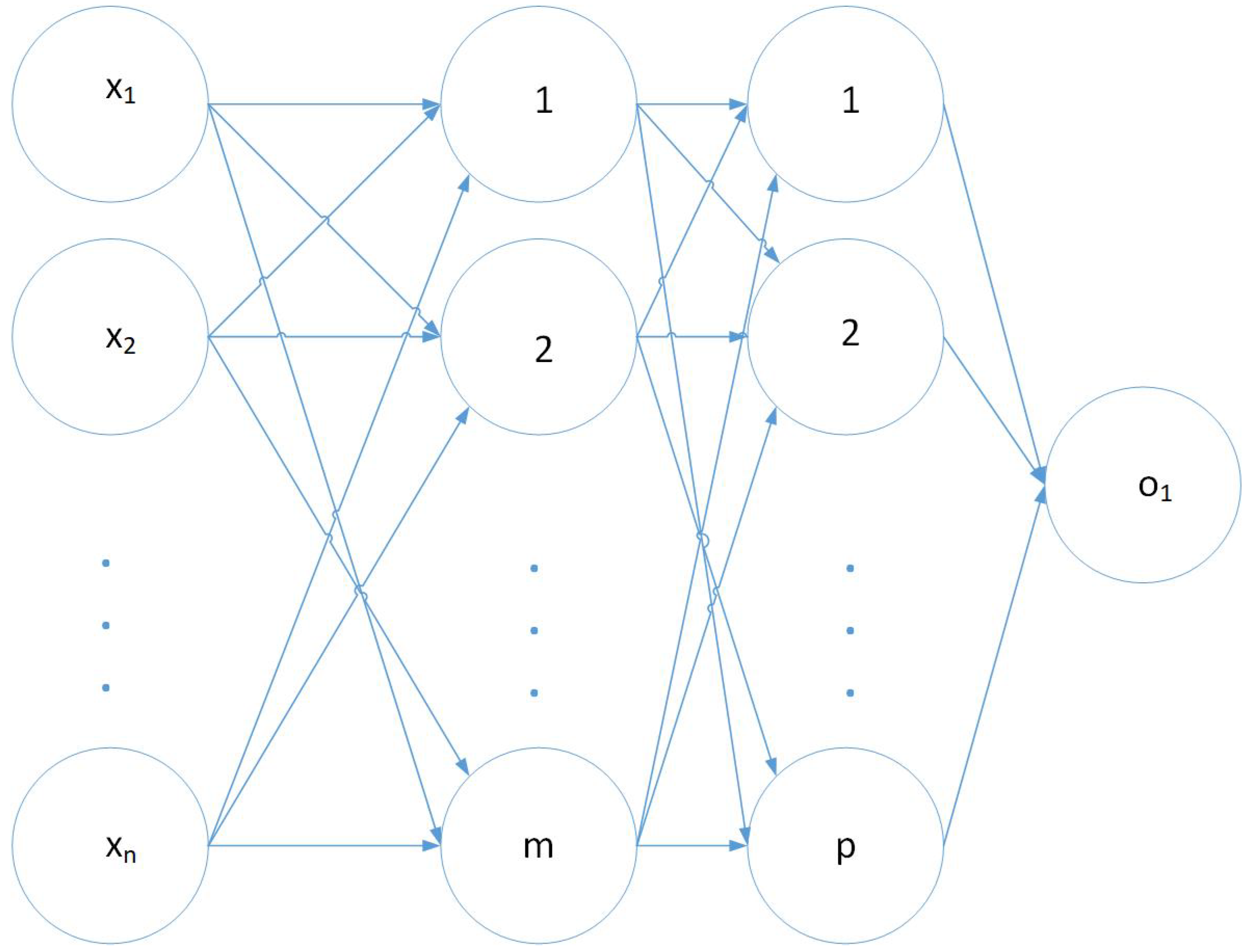
The FFNN architecture is depicted in Figure 1.

Where m is the number of hidden units in the first hidden layer, and p is the number of units in the second hidden layer. This is the simplest deep learning architecture. The mathematical formulation for the l-th hidden layer is expressed as follows [40]:

$$h^{\left(l\right)}={\sigma }^{\left(l\right)}(W^{\left(l\right)T}·x^{\left(l\right)}+b^{\left(l\right)})$$

(1)

where $\sigma$ represents the activation function, W is the weight matrix combining the input x and $h^{\left(1\right)}$ is the output of the first hidden unit, respectively, and b is the bias term. It is worth noting that it is the activation function that introduces the non-linearity behavior into the FFNN modeling. During the training period, the training algorithm adjusts the weights and biases iteratively to minimize the error between actual and predicted values of the ANN model. A set of input and output data is called a training set of data. The input data sets are trained by learning algorithms. This training process is repeated until the error reduces to an acceptable value [41].

2.2. Recurrent Neural Networks

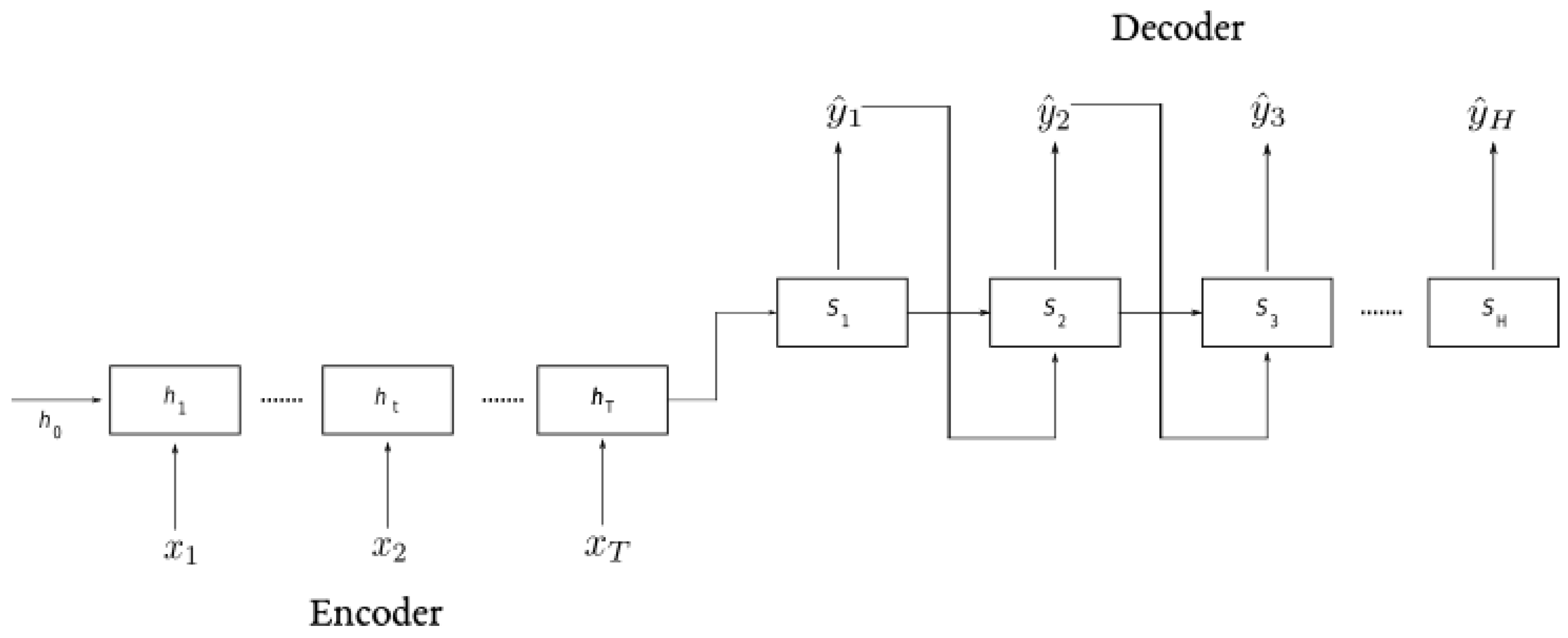
Recurrent neural networks (RNN) are a family of neural networks for processing sequential data. They can scale to process very long sequences as well as variable length [40]. The RNN architecture used in this work is called sequence to sequence and is depicted in Figure 2. A complete description of this recurrent neural network architecture can be found in [33].

This work employs LSTM cells, which are a type of RNN unit that avoids the vanishing gradient. The complete mathematical formulation for this type of recurrent unit is as follows:

$$\begin{array}{cc}\hfill i_t& =\sigma (W_i·h_{t-1}+V_i·x_t+P_i·C_{t-1}+b_i)\hfill \end{array}$$

(2a)

$$\begin{array}{cc}\hfill o_t& =\sigma (W_0·h_{t-1}+V_0·x_t+P_0·C_t+b_0)\hfill \end{array}$$

(2b)

$$\begin{array}{cc}\hfill f_t& =\sigma (W_f·h_{t-1}+V_f·x_t+P_f·C_{t-1}+b_f)\hfill \end{array}$$

(2c)

$$\begin{array}{cc}\hfill \widehat{C_t}& =tanh(W_c·h_{t-1}+V_c·x_t+b_c)\hfill \end{array}$$

(2d)

$$\begin{array}{cc}\hfill C_t& =i_t\odot \widehat{C_t}+f_t\odot C_{t-1}\hfill \end{array}$$

(2e)

$$\begin{array}{cc}\hfill h_t& =o_t\odot tanh\left(C_t\right)\hfill \end{array}$$

(2f)

$$\begin{array}{cc}\hfill z_t& =h_t\hfill \end{array}$$

(2g)

where i, o, and f correspond to the input, output, and forget gate. W and V are the weight matrices linked to the hidden states and inputs, respectively. Moreover, the ⊙ symbol represents the operation of element-wise multiplication. The LSTM cell has two states: the hidden state $h_t$ and the internal cell state $C_t$. $\widehat{C_t}$ is the current candidate to the cell state at period t. The input and forget gates determine how much of past information should be retained, whereas the output gate determines the present hidden state that will be passed to the next LSTM unit. $z_t$ determines the output of the cell, which in this case is equal to the hidden state $h_t$ [42].

During back-propagation, only the forecasts produced from the decoder are considered as follows:

$$E=\sum _{t=1}^H{A}_t-F_t$$

(3)

2.3. Benchmark Methods

Seasonal-naive, exponential smoothing and ARIMA methods were employed as baseline methods to compare the deep learning models’ performance. To get a sense of how good the performance of our deep learning models are, we employ the following metrics: mean absolute scaled error (MASE), mean absolute error (MAE), root mean squared error (RMSE), weight average percentage error (WAPE), and absolute percentage bias (APB).

$$\begin{array}{cc}\hfill MASE& =\frac{\frac{{\sum }_{t=1}^H|A_t-F_t|}{H}}{\frac{{\sum }_{t=m+1}^H|A_t-A_{t-m}|}{H-m}}\hfill \end{array}$$

(4)

$$\begin{array}{cc}\hfill MAE& =\sum _{t=1}^H\frac{(A_t-F_t)}{H}\hfill \end{array}$$

(5)

$$\begin{array}{cc}\hfill RMSE& =\sqrt{\frac{{\sum }_{t=1}^H{(A_t-F_t)}^2}{H}}\hfill \end{array}$$

(6)

$$\begin{array}{cc}\hfill WAPE& =\frac{{\sum }_{t=1}^H|A_t-F_t|}{{\sum }_{t=1}^H|A_t|}\hfill \end{array}$$

(7)

$$\begin{array}{cc}\hfill APB& =\frac{{\sum }_{t=1}^H|A_t-F_t|}{{\sum }_{t=1}^H{A}_t}\times 100\hfill \end{array}$$

(8)

where A is the observed value, F is the forecasted value, n is the train set length, H is the forecasting horizon, and m is the seasonal period. All of these metrics are commonly found in the literature when evaluating forecasting performance. Nevertheless, in GHI predictions for microgrids design, we consider WAPE as an excellent evaluator: it is symmetric, which means it does not differentiate whether the forecast is over-predicted or under-predicted; it is more robust than RMSE since it employs the absolute error instead of the squared error; and it is not affected by low values (close to zero).

3. Case Study

For this paper, we take into account historical GHI data collected from Michoacan, Mexico. These data are open source, which ensures replicability of the presented results.

Data were acquired by using the API provided by the National Renewable Energy Laboratory. This API enabled to obtain data collected from a solar station located at specific coordinates in the region. The National Solar Radiation Database (NSRDB) is a serially complete collection of hourly and half-hourly values of meteorological data and the three most common measurements of solar radiation: global horizontal, direct normal and diffuse horizontal irradiance.

Using the NSRDB data, it is possible to estimate the amount of solar energy that has been historically available at a given time and location anywhere in the United States; the NSRDB is also expanding to encompass a growing list of international locations [43].

The information of the station is summarized in

Table 1. Station information.

ID	571501
Latitude	19.65
Longitude	−101.66

. In addition to historical data, theoretical values applying GHI clear-sky models were computed.

4. Methodology

In this section, we describe the steps followed to apply deep learning techniques to predict global horizontal irradiance (GHI). As we know, there are three components of solar irradiance: direct, diffuse, and global components. However, this work is focused on the global component since it has been widely used to estimate power generation in photovoltaic technologies [44]. Figure 3 represents the flow diagram with the methodology employed for this work. This methodology is based on the CRISP-DM methodology [45].

The first step was to describe the data acquisition. To this aim, 14 years of historical half-hourly data were collected (from 2007 to 2020). In order to explore the data obtained, a time series decomposition was performed to identify the seasonality, trend, and residual components in the historical data. Analyzing the GHI distribution with respect to the time gives us enough information to get rid of 0 values, which were not considered as part of the forecasting task.

An analysis of clear-sky models was necessary to include not only historical data, but also a variable which adds information to predict GHI. To avoid colinearity, only one clear-sky model was included as an exogenous variable for the models.

Applying deep learning techniques for long-term forecasting requires specific data preparation steps. FFNN and RNN require both different pre-processing, which are explained in Section 5. Then, the fitting of these two models is carried out.

The evaluation part includes the computation of metrics to evaluate the long-term forecast with respect to the observed values of 2020. A grid search procedure is carried out to find good hyperparameters for this forecasting task.

Uncertainty for these models comes from two sources: aleatoric and epidemic [46]. Aleatoric uncertainty has to do with data collection and is irreducible. In this case, it is related to the instruments’ accuracy. On the other hand, epistemic uncertainty occurs due to training data being not appropriate. This kind of uncertainty tends to arise in regions where there are not enough training samples.

Finally, each metric distribution is presented using boxplots to analyze the variability and the median of each deep learning model.

The forecast for each technique corresponds to the average of 10 different forecasts applying a particular random seed to avoid a bias caused by some extraordinary result generated by a “lucky” seed.

5. Analysis of Results

5.1. Data Exploration

As it is shown in Figure 4, historical GHI data have 0 values before 8:00 a.m. and after 19:30 p.m. Then, in this paper, only non-zero values are considered for training and evaluating the models.

A time series decomposition was performed to identify patterns in the historical GHI data. For illustrative purposes, in this section, we only plot our analysis for December 2019. Observed values are depicted in Figure 5.

Whereas there is no a clear pattern for the trend (see Figure 6), the seasonal component shown in Figure 7 seems much stronger. The residual component is depicted in Figure 8.

In order to include more information about the GHI, three theoretical models were considered: Ineichen, Haurwitz, and Solis. Although all of them replicate the seasonal pattern observed in the previous exploration, they all present subtle differences with respect to the observed GHI as it is depicted in Figure 9.

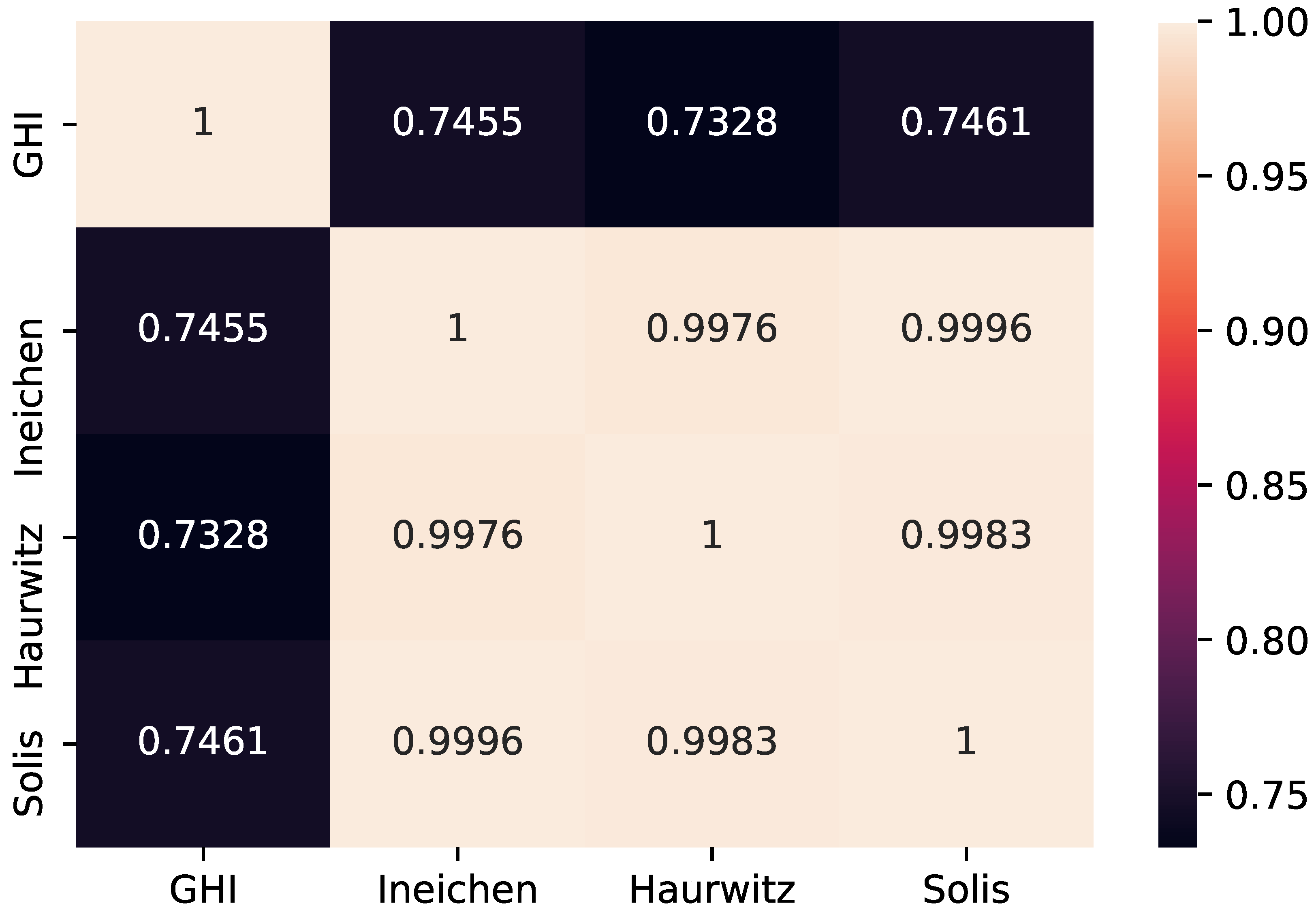
In order to select the most appropriate mathematical model, the correlation matrix shown in Figure 10 is computed to find the one that contributes the most information. Only one of them is selected to avoid problems of colinearity. As it is depicted in Figure 10, the Solis model has the strongest correlation with respect to GHI.

5.2. Data Preparation

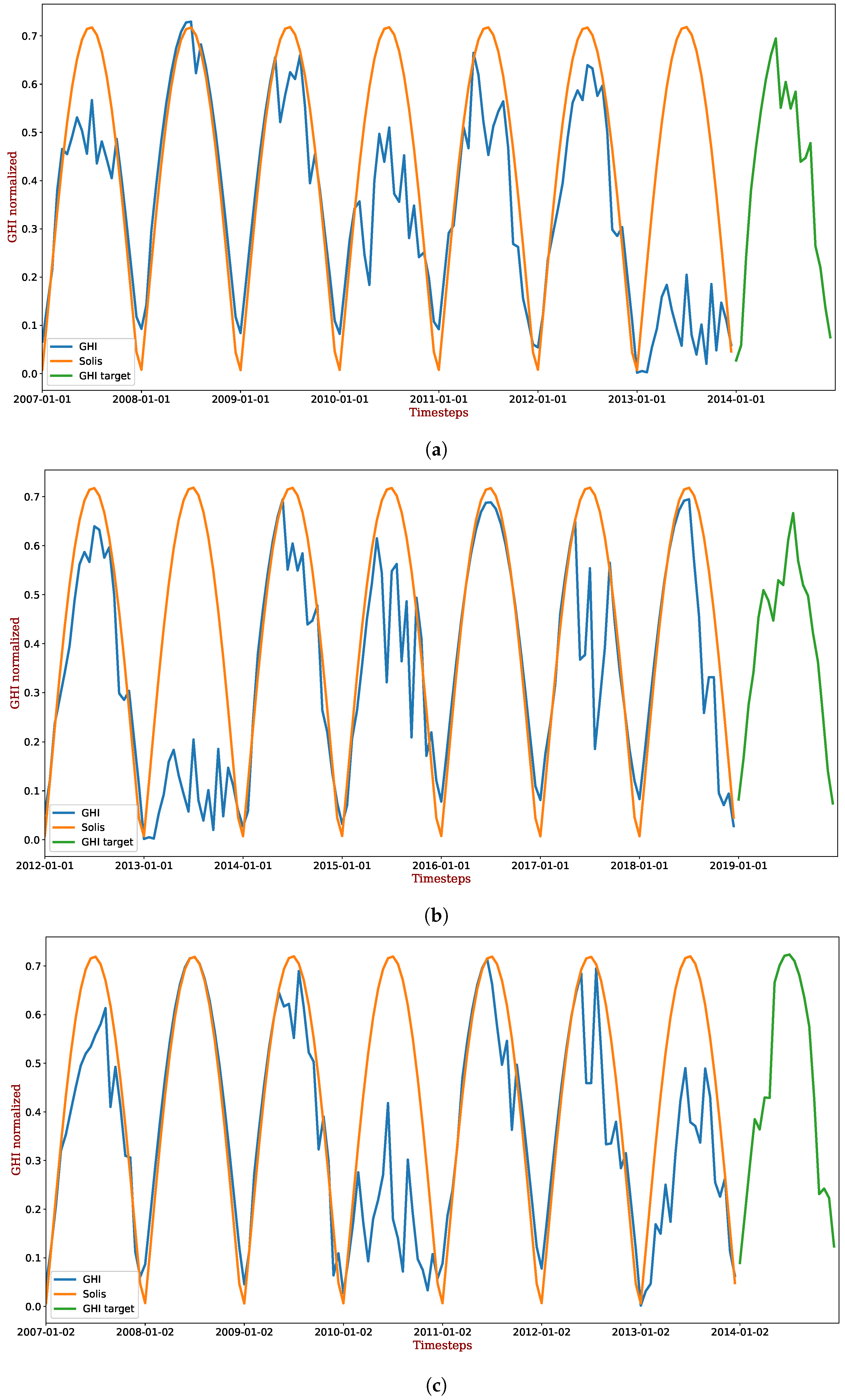
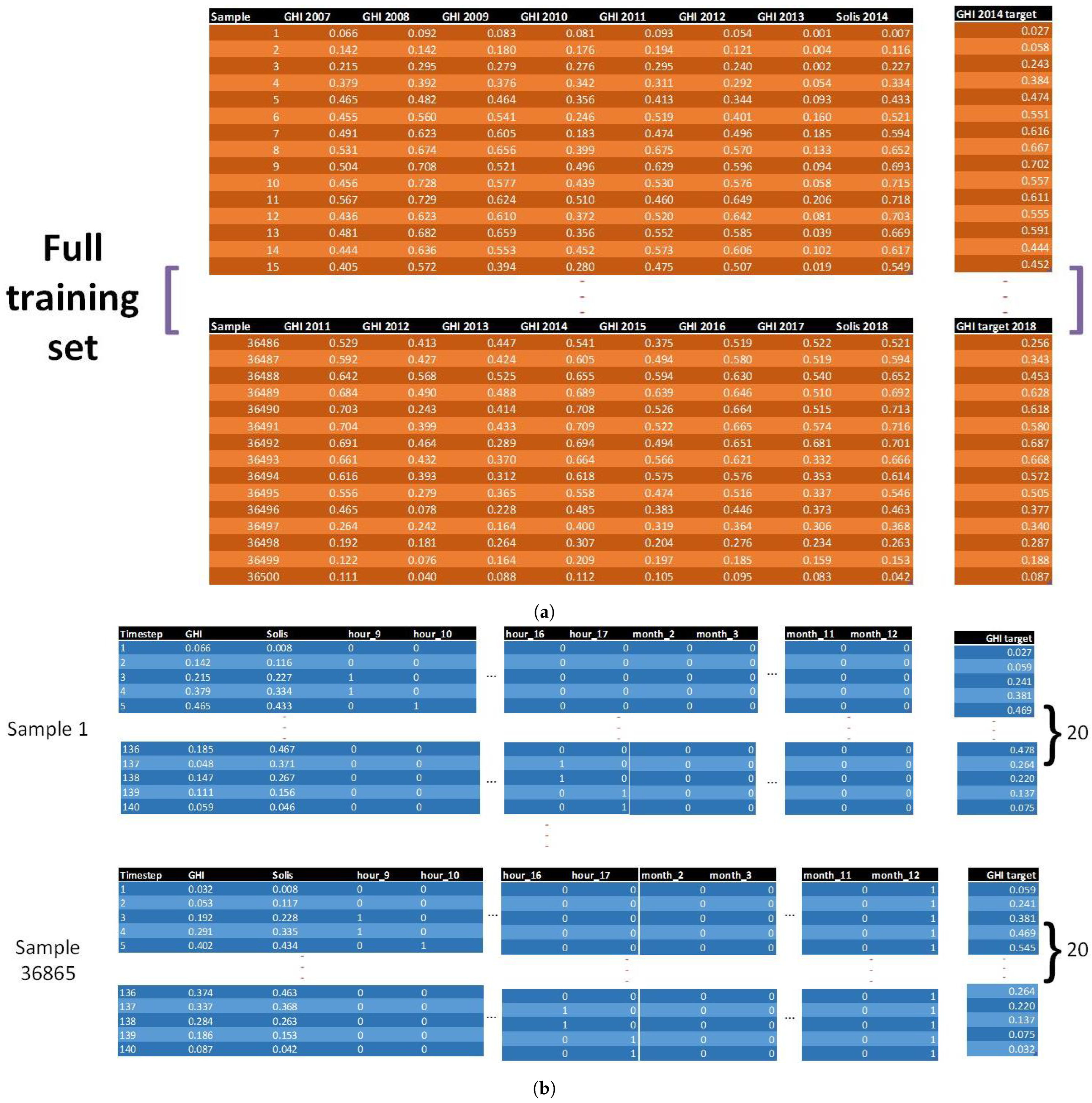
Two different approaches were employed to prepare the data to be used by the FFNN and the RRNN models. The first model requires eight inputs, which correspond to seven measures of GHI at a particular date and the same time but for seven different years. The eighth input is the value given by the Solis model at this particular date and time but for the same year which is predicted (the output). The RNN requires more elaboration in this step. Instead of seven time steps being used as inputs, seven whole days of data from seven consecutive years are employed as inputs. For instance, the first sample in the training set is constituted as follows: it includes the 20 time steps of January 1st for seven consecutive years (see Figure 11a). For each time step, both the observed GHI and the value given by the Solis model are included. Furthermore, dummy variables to indicate the month and hour corresponding to the time step are included (dropping the first element so that co-linearity is avoided). In that way, we increase the capacity of the model to grasp the daily and monthly seasonality from data. Then, each sample for the RNN model is a matrix with 140 rows and 22 columns. The output of the model is a vector of 20 time steps corresponding to January 1st from the year next to the last one included in the input (2014, for the first sample). In this way, it is possible to include daily and not only yearly seasonality into the model. Thus, the FFNN model employs a 2D matrix as input (samples, features), where there are eight features (see Figure 12a). In contrast, the RNN model requires a 3D tensor as input (samples, time steps, and features) where the number of time steps is 140 (7 days with 20 timesteps and 22 features, GHI observed, Solis model, and dummy variables; see Figure 12b). For the latter case, only two features are illustrated in Figure 11a. Figure 11b,c represents the same scheme for samples 101 and 102 to illustrate how the full batch is constituted.

In the case of FFNN, a single supervised learning model is trained with a single output as depicted in Figure 1. This model is then applied 7300 times (365 days × 20 time steps by day). To apply the RNN, the MIMO strategy is employed for this long-term forecasting task (see [47]). This method finds one forecasting model, which computes the forecast for one whole day. The obtained model is then fed 365 times to predict the entire year of GHI.

5.3. Evaluation

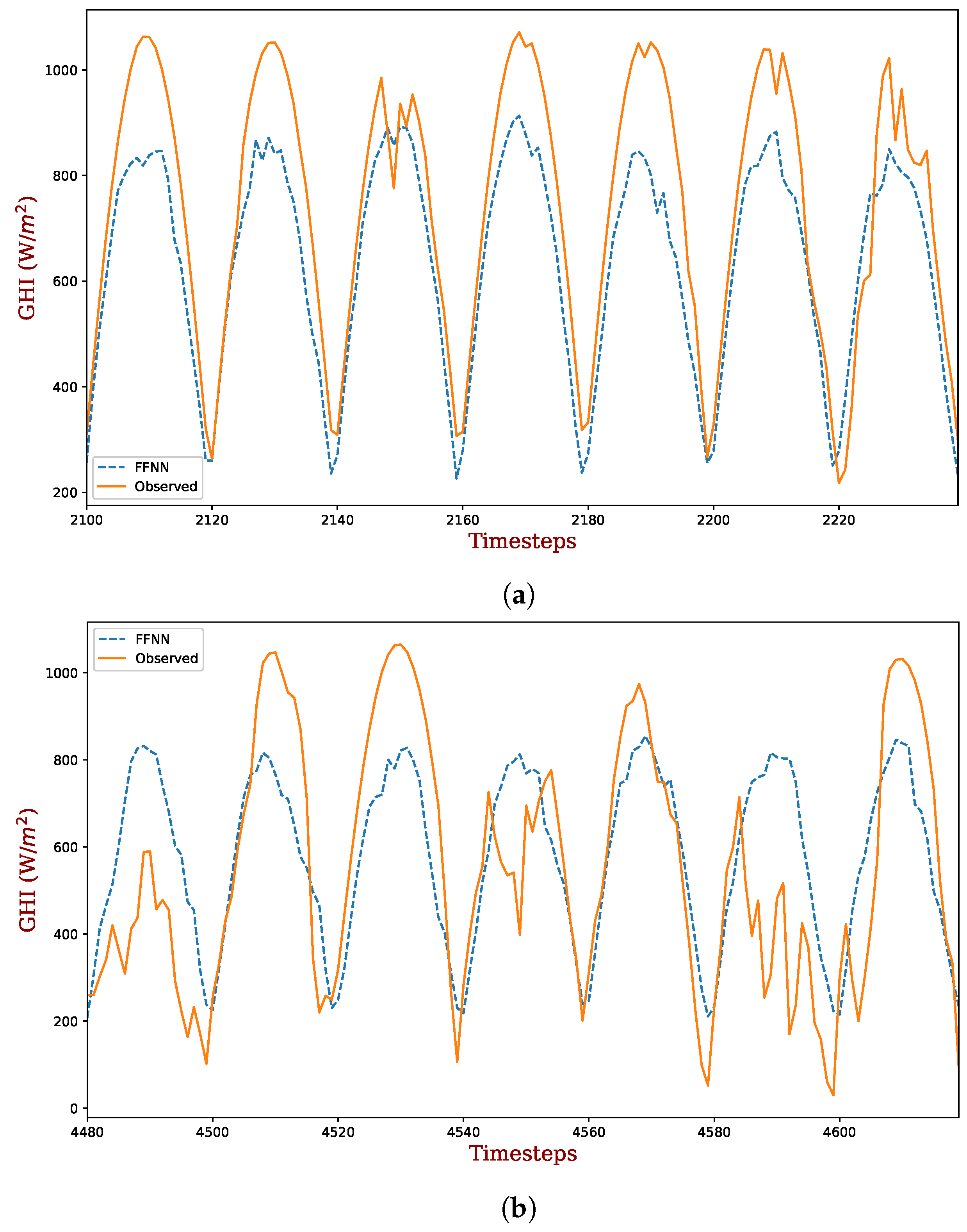
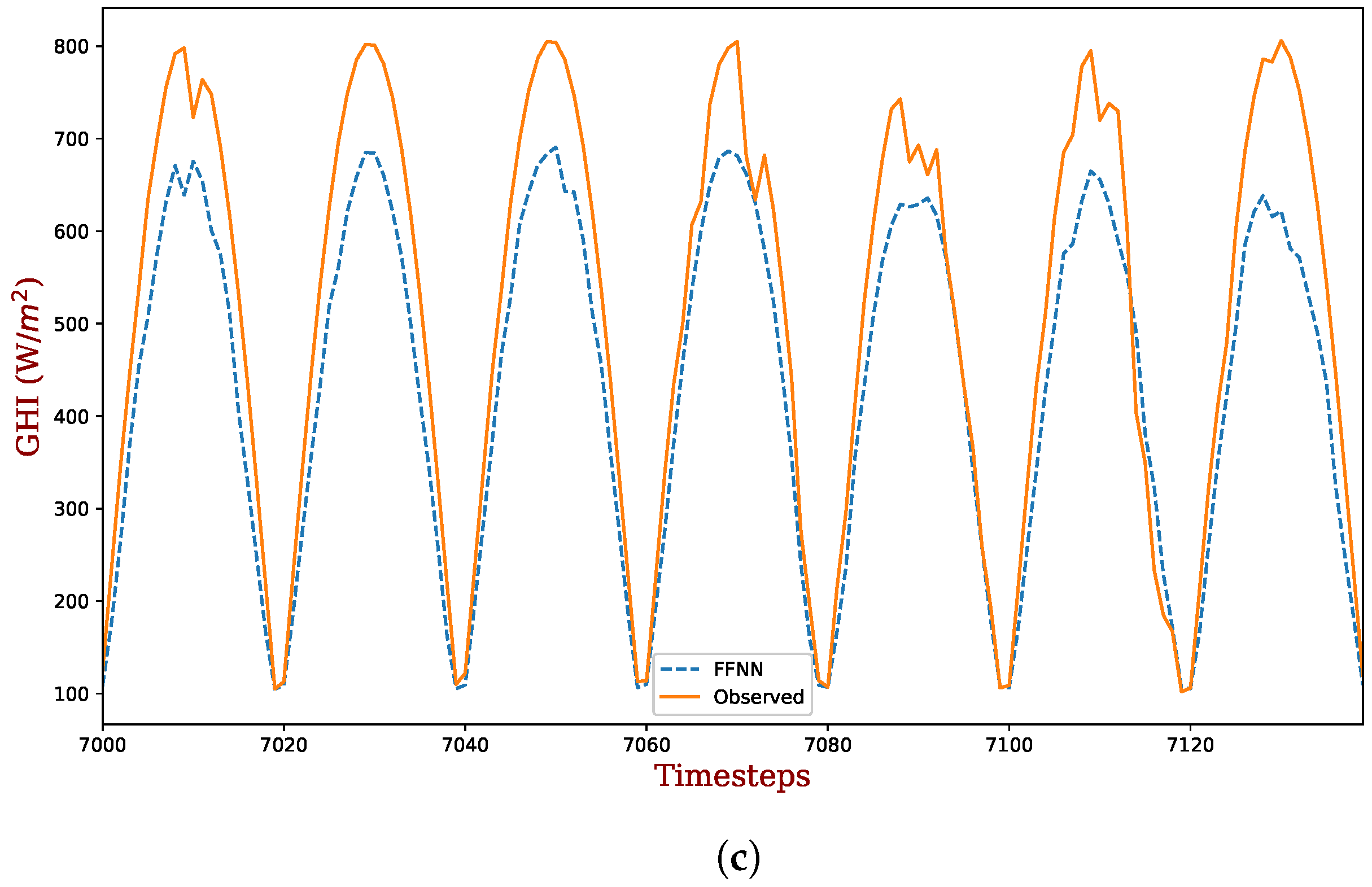
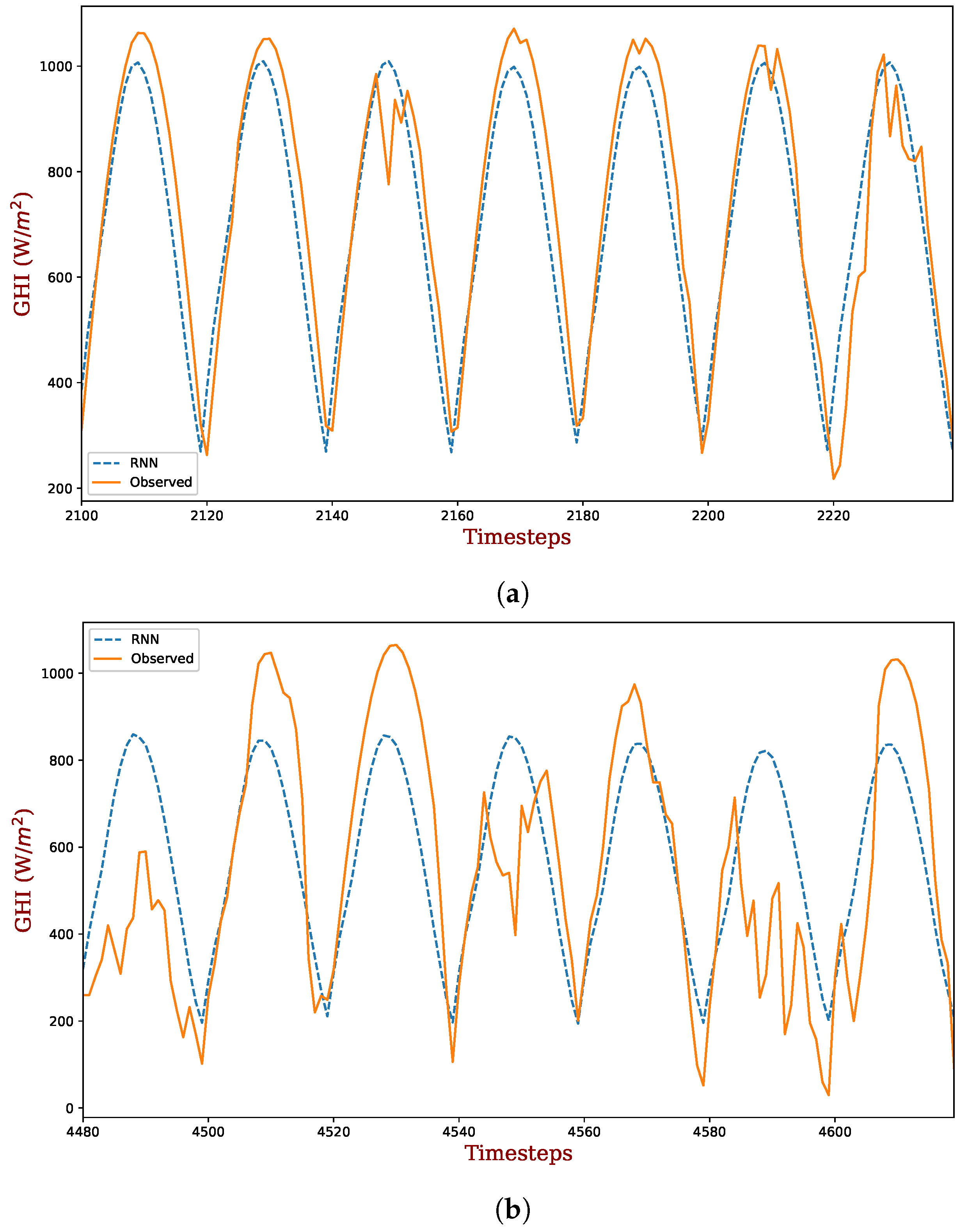
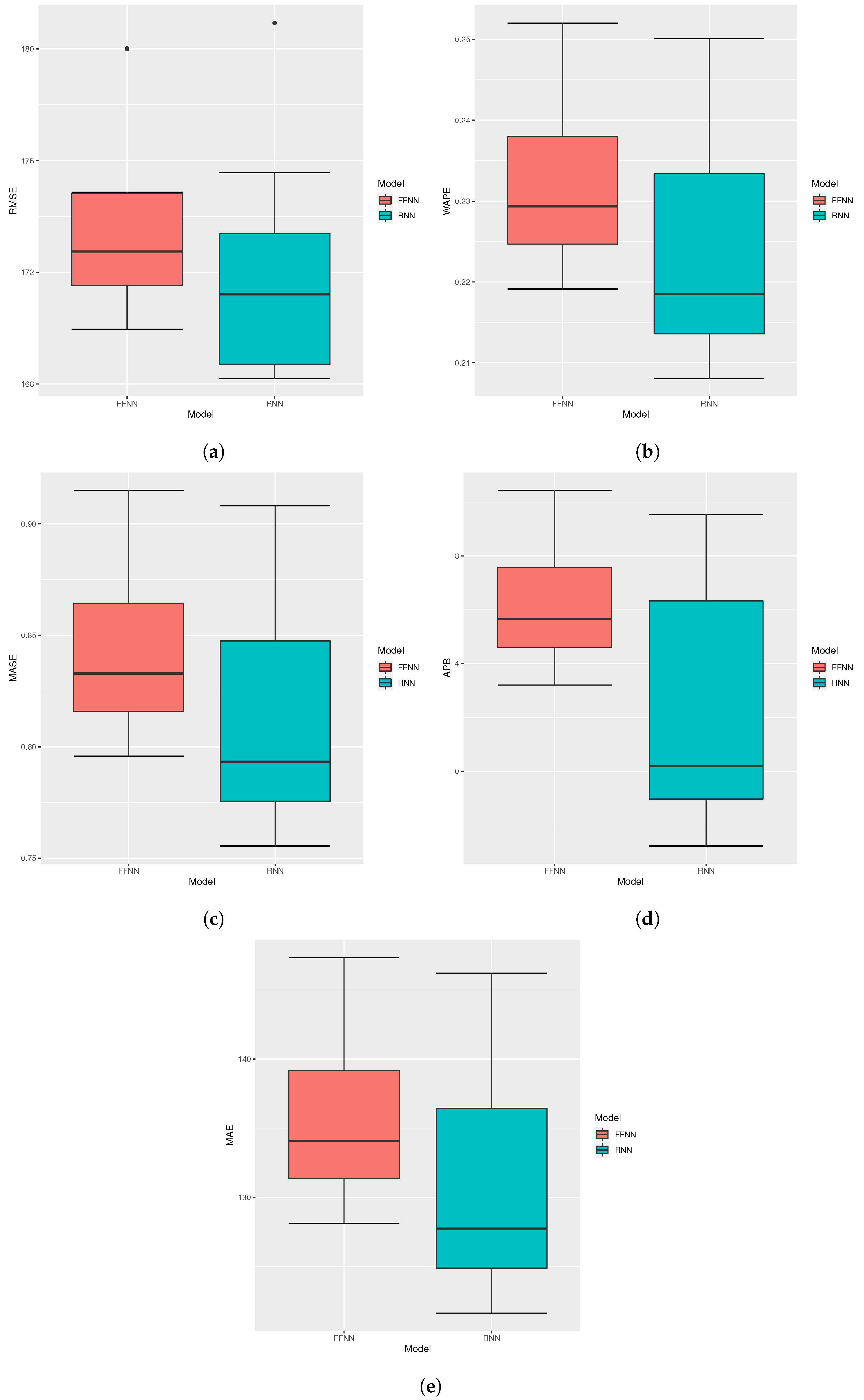
Both deep learning models are evaluated under the same circumstances. In order to avoid a bias from the seed provided by the computational framework (Keras), 20 forecasts are averaged so that the corresponding seed effect is minimized. Figure 13a–c illustrates the performance of FFNN, whereas Figure 14a–c illustrates the performance of RNN in this forecasting task. Weeks 16, 34, and 51 of year 2020 were selected to show how good the forecasting performance of each model is.

Table 2. Hyperparameter values for grid-search.

	Epochs	Batch Size	Units Hidden 1	Units Hidden 2	Units Encoder	Units Decoder	Learning Rate
FFNN	20, 30, 40	256, 512, 1024	128, 256, 512	16, 32, 64	-	-	0.0005, 0.001, 0.01
RNN	40, 80, 120	256, 512, 1024	-	-	16, 32, 64	16, 32, 64	0.0001, 0.001, 0.01

The values in bold correspond to the optimal configuration after carrying out the grid-search procedure.

depicts the values employed for the grid search procedure, where the bold text specifies the optimal values found for the average of 10 runs per combination. Moreover, the median of the forecasting metrics is shown in

Table 3. Baseline and deep learning methods performance.

Metric	Naive	Exp. Smoothing	ARIMA	FFNN	RNN
RMSE	225.817	231.580	218.461	174.728	170.033
WAPE	0.258	0.290	0.308	0.241	0.224
MASE	1.000	1.053	1.117	0.876	0.815
MAE	150.650	169.543	179.851	141.052	131.144
APB	3.067	−15.399	20.470	8.051	2.795

The values in bold correspond to the best metric computation among the forecasting techniques.

. For all the metrics, the proposed RNN approach was better than the FFNN one. In addition to that, both of them performed better than the classical models employed as a baseline (Exponential smoothing, ARIMA, seasonal-naive with yearly seasonality). Figure 15a–e illustrates the range, median, and variability of the computed metrics for each model with 10 random seeds. In general, the end user could expect better performance of RNN over FFNN 50% of the time for WAPE, MAPE, APB, and MAE. In contrast, RNN shows more variability with respect to these four indicators. RMSE is slightly better for RNN than FFNN.

In order to establish statistical significance for these metrics, the non-parametric Mann–Whitney U test was performed (see

Table 4. U-Mann Whitney Test.

	RMSE	WAPE	MASE	APB	MAE
statistic	34	25	25	25	25
p-value	0.121	0.032	0.032	0.032	0.032

The values in bold corresponds to the values that show statistical significance considering a significance level of 5%.

). The alternative hypothesis involves that a run of the RNN model with a random seed obtains a better score over a run of the FFNN model under the same circumstances. As it was suggested by the previous box-plots, RNN obtains a statistically significant advantage over FFNN in terms of WAPE, MAPE, MASE, and MAE.

Table 5. Training and testing time in seconds.

Computational Time	Naive	Exp. Smoothing	ARIMA	FFNN *	RNN *
Training	0.68	12.09	18,421.12	6.02	118.42
Testing	0.01	0.07	3.18	1.05	2.03

shows the average computational time for each model in seconds. FFNN and RNN were run using a GPU NVIDIA GeForce GTX 960M to make the run procedure even faster, whereas the rest of them were run by default with a CPU with the following characteristics: Intel(R) Core(TM) i5-6300HQ @ 2.30 GHz, 8 GB of RAM.

6. Conclusions

Long-term GHI forecasting has been slightly studied in the literature until now. In this work, we propose a new approach to feed two deep learning models to face this task: feed forward neural networks and recurrent neural networks. For each technique, a single model was trained in a very short computational time (less than 3 s in each case). We applied the proposed technique to a case study in Michoacan, Mexico. Data exploration showed that GHI non-zero values were found between 8:00 a.m. and 5:30 p.m. Two different data preparation techniques were employed to feed the inputs to the deep learning models. The clear-sky model “Solis” was employed to enrich historical data and improve the forecasting power of our proposed approaches, given that it provided better correlation with the historical data (0.7461). Three time series forecasting methods (ARIMA), exponential smoothing (ES), and seasonal naive (SN) were used for benchmarking purposes. In terms of RMSE, the two deep learning methods resulted in being more effective (FFNN: 174.728, RNN: 170.033) with respect to the benchmark (S.N.: 225.817, E.S.: 231.580, ARIMA: 218.461). Finally, the Mann–Whitney U test showed that RNN showed significantly better performance over FFNN in terms of WAPE, MAPE, MASE, and MAE (p value of 0.032). In this work, RNN and FFNN were used for long-term forecasting using the proposed approach. However, these two approaches are commonly used for short-term forecasting. Only deep learning models were included in this study. However, for a further comparison, machine learning models, such as support vector machines and random forests will be employed. In addition to that, tensor-train recurrent neural networks, which is a novel and specialized deep learning technique for long-term time series forecasting (see [48]), will also be used to explore its performance facing this task in future work. This work has entailed the GHI forecast as part of a planning problem (considering the desired resolution for microgrids sizing). However, the importance of the optimal control of microgrids has gained importance in the context of smart cities and smart grids, which are part of the internet of things (IIOT) [49]. The study of the challenges related to IIOT and big data in the context of mobile devices includes how to manage and store data (see [50]). Specifically, one alternative to tackle this problem is to reduce the number of parameters to increase the model’s speed of training (see [51]), which will be studied in a next work. The long-term prediction of GHI is vital to achieve a good microgrid design when photovoltaic technologies are included. For future work, we will embed the long-term forecasting methodology in an optimization framework to obtain the optimal design of microgrids.

References

1. IEA. World Energy Outlook 2020. Available online: https://www.iea.org/reports/world-energy-outlook-2020 (accessed on 1 December 2021).
2. IEA. Tracking SDG 7: The Energy Progress Report 2019. Available online: https://www.irena.org/publications/2019/May/Tracking-SDG7-The-Energy-Progress-Report-2019 (accessed on 1 December 2021).
3. Medina-Santana, A.A.; Flores-Tlacuahuac, A.; Cárdenas-Barrón, L.E.; Fuentes-Cortés, L.F. Optimal design of the water-energy-food nexus for rural communities. Comput. Chem. Eng. 2020, 143, 107120. [Google Scholar] [CrossRef]
4. Rodriguez, M.; Espin, V.; Arcos-Aviles, D.; Martinez, W. Energy management system for an isolated microgrid based on Fuzzy logic control and meta-heuristic algorithms. In Proceedings of the 2022 IEEE 31st International Symposium on Industrial Electronics (ISIE), Anchorage, AK, USA, 1–3 June 2022; pp. 462–467. [Google Scholar]
5. Emad, D.; El-Hameed, M.; Yousef, M.; El-Fergany, A. Computational methods for optimal planning of hybrid renewable microgrids: A comprehensive review and challenges. Arch. Comput. Methods Eng. 2020, 27, 1297–1319. [Google Scholar] [CrossRef]
6. Yuan, H.; Ye, H.; Chen, Y.; Deng, W. Research on the optimal configuration of photovoltaic and energy storage in rural microgrid. Energy Rep. 2022, 8, 1285–1293. [Google Scholar] [CrossRef]
7. Das, B.K.; Al-Abdeli, Y.M.; Kothapalli, G. Optimisation of stand-alone hybrid energy systems supplemented by combustion-based prime movers. Appl. Energy 2017, 196, 18–33. [Google Scholar] [CrossRef]
8. Kamal, M.M.; Ashraf, I.; Fernandez, E. Planning and optimization of microgrid for rural electrification with integration of renewable energy resources. J. Energy Storage 2022, 52, 104782. [Google Scholar] [CrossRef]
9. Lan, H.; Wen, S.; Hong, Y.Y.; David, C.Y.; Zhang, L. Optimal sizing of hybrid PV/diesel/battery in ship power system. Appl. Energy 2015, 158, 26–34. [Google Scholar] [CrossRef]
10. Abd el Motaleb, A.M.; Bekdache, S.K.; Barrios, L.A. Optimal sizing for a hybrid power system with wind/energy storage based in stochastic environment. Renew. Sustain. Energy Rev. 2016, 59, 1149–1158. [Google Scholar] [CrossRef]
11. Abualigah, L.; Zitar, R.A.; Almotairi, K.H.; Hussein, A.M.; Abd Elaziz, M.; Nikoo, M.R.; Gandomi, A.H. Wind, solar, and photovoltaic renewable energy systems with and without energy storage optimization: A survey of advanced machine learning and deep learning techniques. Energies 2022, 15, 578. [Google Scholar] [CrossRef]
12. Al-Falahi, M.D.; Jayasinghe, S.; Enshaei, H. A review on recent size optimization methodologies for standalone solar and wind hybrid renewable energy system. Energy Convers. Manag. 2017, 143, 252–274. [Google Scholar] [CrossRef]
13. Kusakana, K.; Vermaak, H.; Numbi, B. Optimal sizing of a hybrid renewable energy plant using linear programming. In Proceedings of the IEEE Power and Energy Society Conference and Exposition in Africa: Intelligent Grid Integration of Renewable Energy Resources (PowerAfrica), Johannesburg, South Africa, 9–13 July 2012; pp. 1–5. [Google Scholar]
14. Domenech, B.; Ranaboldo, M.; Ferrer-Martí, L.; Pastor, R.; Flynn, D. Local and regional microgrid models to optimise the design of isolated electrification projects. Renew. Energy 2018, 119, 795–808. [Google Scholar] [CrossRef]
15. Khatod, D.K.; Pant, V.; Sharma, J. Analytical approach for well-being assessment of small autonomous power systems with solar and wind energy sources. IEEE Trans. Energy Convers. 2009, 25, 535–545. [Google Scholar] [CrossRef]
16. Luna-Rubio, R.; Trejo-Perea, M.; Vargas-Vázquez, D.; Ríos-Moreno, G. Optimal sizing of renewable hybrids energy systems: A review of methodologies. Sol. Energy 2012, 86, 1077–1088. [Google Scholar] [CrossRef]
17. Nadjemi, O.; Nacer, T.; Hamidat, A.; Salhi, H. Optimal hybrid PV/wind energy system sizing: Application of cuckoo search algorithm for Algerian dairy farms. Renew. Sustain. Energy Rev. 2017, 70, 1352–1365. [Google Scholar] [CrossRef]
18. Suman, G.K.; Guerrero, J.M.; Roy, O.P. Optimisation of solar/wind/bio-generator/diesel/battery based microgrids for rural areas: A PSO-GWO approach. Sustain. Cities Soc. 2021, 67, 102723. [Google Scholar] [CrossRef]
19. Bahramara, S.; Moghaddam, M.P.; Haghifam, M. Optimal planning of hybrid renewable energy systems using HOMER: A review. Renew. Sustain. Energy Rev. 2016, 62, 609–620. [Google Scholar] [CrossRef]
20. Lambert, T.W.; Hittle, D. Optimization of autonomous village electrification systems by simulated annealing. Sol. Energy 2000, 68, 121–132. [Google Scholar] [CrossRef]
21. Singla, P.; Duhan, M.; Saroha, S. A comprehensive review and analysis of solar forecasting techniques. Front. Energy 2021, 16, 187–223. [Google Scholar] [CrossRef]
22. Kim, H.; Aslam, M.; Choi, M.; Lee, S. A study on long-term solar radiation forecasting for PV in microgrid. In Proceedings of the APAP Conference, Jeju, Korea, 16–19 October 2017; pp. 16–19. [Google Scholar]
23. Cannizzaro, D.; Aliberti, A.; Bottaccioli, L.; Macii, E.; Acquaviva, A.; Patti, E. Solar radiation forecasting based on convolutional neural network and ensemble learning. Expert Syst. Appl. 2021, 181, 115167. [Google Scholar] [CrossRef]
24. Patterson, J.; Gibson, A. Deep Learning: A Practitioner’s Approach; O’Reilly Media, Inc.: Sebastopol, CA, USA, 2017. [Google Scholar]
25. Bishop, C.M.; Nasrabadi, N.M. Pattern Recognition and Machine Learning; Springer: Berlin/Heidelberg, Germany, 2006; Volume 4. [Google Scholar]
26. Kumar, N.M.; Subathra, M. Three years ahead solar irradiance forecasting to quantify degradation influenced energy potentials from thin film (a-Si) photovoltaic system. Results Phys. 2019, 12, 701–703. [Google Scholar] [CrossRef]
27. Aslam, M.; Lee, J.M.; Kim, H.S.; Lee, S.J.; Hong, S. Deep learning models for long-term solar radiation forecasting considering microgrid installation: A comparative study. Energies 2019, 13, 147. [Google Scholar] [CrossRef] [Green Version]
28. Sharika, W.; Fernando, L.; Kanagasundaram, A.; Valluvan, R.; Kaneswaran, A. Long-term Solar Irradiance Forecasting Approaches—A Comparative Study. In Proceedings of the 2018 IEEE International Conference on Information and Automation for Sustainability (ICIAfS), Colombo, Sri Lanka, 21–22 December 2018; pp. 1–6. [Google Scholar]
29. Aslam, M.; Seung, K.H.; Lee, S.J.; Lee, J.M.; Hong, S.; Lee, E.H. Long-term Solar Radiation Forecasting using a Deep Learning Approach-GRUs. In Proceedings of the 2019 IEEE 8th International Conference on Advanced Power System Automation and Protection (APAP), Xi’an, China, 21–24 October 2019; pp. 917–920. [Google Scholar]
30. Kumar Barik, A.; Malakar, S.; Goswami, S.; Ganguli, B.; Sen Roy, S.; Chakrabarti, A. Analysis of GHI Forecasting Using Seasonal ARIMA. In Data Management, Analytics and Innovation; Springer: Berlin/Heidelberg, Germany, 2021; pp. 55–69. [Google Scholar]
31. Abubakr, M.; Akoush, B.; Khalil, A.; Hassan, M.A. Unleashing deep neural network full potential for solar radiation forecasting in a new geographic location with historical data scarcity: A transfer learning approach. Eur. Phys. J. Plus 2022, 137, 474. [Google Scholar] [CrossRef]
32. Smyl, S. A hybrid method of exponential smoothing and recurrent neural networks for time series forecasting. Int. J. Forecast. 2020, 36, 75–85. [Google Scholar] [CrossRef]
33. Hewamalage, H.; Bergmeir, C.; Bandara, K. Recurrent neural networks for time series forecasting: Current status and future directions. Int. J. Forecast. 2021, 37, 388–427. [Google Scholar] [CrossRef]
34. Ghimire, S.; Deo, R.C.; Raj, N.; Mi, J. Deep solar radiation forecasting with convolutional neural network and long short-term memory network algorithms. Appl. Energy 2019, 253, 113541. [Google Scholar] [CrossRef]
35. Zhang, W.; Maleki, A.; Rosen, M.A. A heuristic-based approach for optimizing a small independent solar and wind hybrid power scheme incorporating load forecasting. J. Clean. Prod. 2019, 241, 117920. [Google Scholar] [CrossRef]
36. Zhang, W.; Maleki, A.; Rosen, M.A.; Liu, J. Sizing a stand-alone solar-wind-hydrogen energy system using weather forecasting and a hybrid search optimization algorithm. Energy Convers. Manag. 2019, 180, 609–621. [Google Scholar] [CrossRef]
37. Gupta, R.; Kumar, R.; Bansal, A.K. BBO-based small autonomous hybrid power system optimization incorporating wind speed and solar radiation forecasting. Renew. Sustain. Energy Rev. 2015, 41, 1366–1375. [Google Scholar] [CrossRef]
38. Maleki, A.; Khajeh, M.G.; Rosen, M.A. Weather forecasting for optimization of a hybrid solar-wind–powered reverse osmosis water desalination system using a novel optimizer approach. Energy 2016, 114, 1120–1134. [Google Scholar] [CrossRef]
39. Benidis, K.; Rangapuram, S.S.; Flunkert, V.; Wang, Y.; Maddix, D.; Turkmen, C.; Gasthaus, J.; Bohlke-Schneider, M.; Salinas, D.; Stella, L.; et al. Deep Learning for Time Series Forecasting: Tutorial and Literature Survey. ACM Comput. Surv. CSUR 2018. [Google Scholar] [CrossRef]
40. Heaton, J. Ian goodfellow, yoshua bengio, and aaron courville: Deep learning. Genet. Program. Evolvable Mach. 2018, 19, 305–307. [Google Scholar] [CrossRef] [Green Version]
41. Ghritlahre, H.K.; Prasad, R.K. Exergetic performance prediction of solar air heater using MLP, GRNN and RBF models of artificial neural network technique. J. Environ. Manag. 2018, 223, 566–575. [Google Scholar] [CrossRef] [PubMed]
42. Feng, Z.K.; Huang, Q.Q.; Niu, W.J.; Yang, T.; Wang, J.Y.; Wen, S.P. Multi-step-ahead solar output time series prediction with gate recurrent unit network using data decomposition and cooperation search algorithm. Energy 2022, 261, 125217. [Google Scholar] [CrossRef]
43. IEA. National Solar Radiation Database. 2021. Available online: https://nsrdb.nrel.gov/ (accessed on 1 January 2022).
44. Gbémou, S.; Eynard, J.; Thil, S.; Guillot, E.; Grieu, S. A Comparative Study of Machine Learning-Based Methods for Global Horizontal Irradiance Forecasting. Energies 2021, 14, 3192. [Google Scholar] [CrossRef]
45. Schröer, C.; Kruse, F.; Gómez, J.M. A systematic literature review on applying CRISP-DM process model. Procedia Comput. Sci. 2021, 181, 526–534. [Google Scholar] [CrossRef]
46. Abdar, M.; Pourpanah, F.; Hussain, S.; Rezazadegan, D.; Liu, L.; Ghavamzadeh, M.; Fieguth, P.; Cao, X.; Khosravi, A.; Acharya, U.R.; et al. A review of uncertainty quantification in deep learning: Techniques, applications and challenges. Inf. Fusion 2021, 76, 243–297. [Google Scholar] [CrossRef]
47. Taieb, S.B.; Bontempi, G.; Atiya, A.F.; Sorjamaa, A. A review and comparison of strategies for multi-step ahead time series forecasting based on the NN5 forecasting competition. Expert Syst. Appl. 2012, 39, 7067–7083. [Google Scholar] [CrossRef]
48. Yu, R.; Zheng, S.; Anandkumar, A.; Yue, Y. Long-Term Forecasting Using Higher Order Tensor RNNs. arXiv 2017, arXiv:1711.00073. [Google Scholar]
49. Kumar, R.L.; Khan, F.; Kadry, S.; Rho, S. A survey on blockchain for industrial internet of things. Alex. Eng. J. 2022, 61, 6001–6022. [Google Scholar] [CrossRef]
50. Khalil, M.I.; Kim, R.; Seo, C. Challenges and opportunities of big data. J. Platf. Technol. 2020, 8, 3–9. [Google Scholar]
51. Han, Y.; Hong, B.W. Deep learning based on fourier convolutional neural network incorporating random kernels. Electronics 2021, 10, 2004. [Google Scholar] [CrossRef]
Figure 1. Feed forward neural network architecture.
Designs 06 00083 g001
Figure 2. Sequence-to-sequence RNN architecture.
Designs 06 00083 g002
Figure 3. Flow diagram of the methodology.
Designs 06 00083 g003
Figure 4. Boxplot for every intra-day time step from 2007 to 2019.
Designs 06 00083 g004
Figure 5. Observed GHI for December 2019.
Designs 06 00083 g005
Figure 6. Trend component of GHI for December 2019.
Designs 06 00083 g006
Figure 7. Seasonal component of GHI for December 2019.
Designs 06 00083 g007
Figure 8. Residual component of GHI for December 2019.
Designs 06 00083 g008
Figure 9. Observed GHI and clear-sky estimation for a particular date.
Designs 06 00083 g009
Figure 10. Correlation matrix between GHI and clear sky models.
Designs 06 00083 g010
Figure 11. Three different samples to feed RNN model after data preparation. (a) First sample in training set. (b) Sample 101 in training set. (c) Sample 102 in training set.
Designs 06 00083 g011
Figure 12. Different schemes to feed the data. (a) A scheme of training set for FFNN model. (b) A scheme of training set for RNN model.
Designs 06 00083 g012
Figure 13. Prediction for three weeks of 2020 with FFNN. (a) Week 16 FFNN. (b) Week 33 FFNN. (c) Week 51 FFNN.
Designs 06 00083 g013aDesigns 06 00083 g013b
Figure 14. Prediction for three weeks of 2020 with RNN. (a) Week 16 RNN. (b) Week 33 RNN. (c) Week 51 RNN.
Designs 06 00083 g014aDesigns 06 00083 g014b
Figure 15. Evaluation of metrics for deep learning models. (a) RMSE for FFNN and RNN. (b) WAPE for FFNN and RNN. (c) MASE for FFNN and RNN. (d) APB for FFNN and RNN. (e) MAE for FFNN and RNN.
Designs 06 00083 g015