A New Approach to Off-Line Robust Model Predictive Control for Polytopic Uncertain Models

School of Electrical and Electronic Engineering, Shanghai Institute of Technology, Shanghai 201418, China
*
Authors to whom correspondence should be addressed.
Designs 2018, 2(3), 31; https://doi.org/10.3390/designs2030031
Submission received: 9 July 2018
/
Revised: 25 July 2018
/
Accepted: 6 August 2018
/
Published: 20 August 2018
Abstract
:Concerning the robust model predictive control (MPC) for constrained systems with polytopic model characterization, some approaches have already been given in the literature. One famous approach is an off-line MPC, which off-line finds a state-feedback law sequence with corresponding ellipsoidal domains of attraction. Originally, each law in the sequence was calculated by fixing the infinite horizon control moves as a single state feedback law. This paper optimizes the feedback law in the larger ellipsoid, foreseeing that, if it is applied at the current instant, then better feedback laws in the smaller ellipsoids will be applied at the following time. In this way, the new approach achieves a larger domain of attraction and better control performance. A simulation example shows the effectiveness of the new technique.
1. Introduction
Model predictive control (MPC) has attracted considerable attention, since it is an effective control algorithm to deal with multivariable constrained control problems. The nominal MPC for constrained linear systems has been solved in systematic ways around 2000 [1,2]. Recently, some approaches have been extended to distributed implementations [3,4]. Synthesizing robust MPC for constrained uncertain systems has attracted great attention after the nominal MPC. This has become a significant branch of MPC. The lack of robustness in MPC, based on a nominal model [5], calls for a robust MPC technique based on uncertainty models. Up to now, robust MPC has been solved in several ways [6,7,8]. A good technique for robust MPC, however, requires not only guaranteed stability, but also low computational burden, big (at least desired) domain of attraction, and low performance cost value [9].
The authors in [6] firstly solved a min-max optimization problem in an infinite horizon for systems with polytopic description, by fixing the control moves as a state feedback law that was on-line calculated. The authors in [9] off-line calculated a feedback law sequence with corresponding ellipsoidal domains of attraction, and on-line interpolated the control law at each sampling time applying this sequence. The computational burden is largely reduced. In addition, nominal performance cost is used in [9] to the take place of the “worst-case” one so that feasibility can be improved. A heuristic varying-horizon formulation is used and the feedback gains can be obtained in a backward manner.
In this paper, the off-line technique in [9] is further studied. Originally, each off-line feedback law was calculated where the infinite horizon control move was treated as a single state feedback law. This paper, instead, optimizes the feedback law in the larger ellipsoid by considering that the feedback laws in the smaller ellipsoids will be applied at the next time if it is applied at the current time. In a sense, the new technique in this paper is equivalent to a varying-horizon MPC, i.e., the control horizon (say ) gradually changes from M > 1 to M = 1, while the technique in [9] can be taken as a fixed horizon MPC with M = 1. Hence, the new technique achieves better control performance and can control a wider class of systems, i.e., improve control performance and feasibility.
So far, the state feedback approach is popular in most of the robust MPC problem, and the full state is assumed to be exactly measured to act as the initial condition for future predictions [10,11,12,13,14]. However, in many control problems, not all states can be measured exactly, and only the output information is available for feedback. In this case, an output feedback RMPC design is necessary (e.g., [3,15]). The output feedback MPC approach, parallel to that in [6], has been proposed in [16], and the off-line robust MPC has been studied in [17]. The new approach in this paper may be applied to improve the procedure in [17], which will be studied in the near future.
Notation: The notations are fairly standard. is the -dimensional space of real valued vectors. W > 0 (W ≥ 0) means that W is symmetric positive-definite (symmetric non-negative-definite). For a vector x and positive-definite matrix , . is the value of vector x at a future time k + i predicted at time k. The symbol * induces a symmetric structure, e.g., when and are symmetric matrices, then .
2. Problem Statement
Consider the following time varying model:
with input and state constraints, i.e.,
where and are input and measurable state, respectively; , and with , and , ; . Input constraint is common in practice, which arises from physical and technological limitations. It is well known that the negligence of control input constraints usually leads to limit cycles, parasitic equilibrium points, or even causes instability. Moreover, we assume that , where , i.e., there exist nonnegative coefficients , such that
A predictive controller is proposed to drive systems (1) and (2) to the origin , and at each time , to solve the following optimization problem:
The following constraints are imposed on Equation (4a):
for all i ≥ 0. In (4), and are weighting matrices and are the decision variables. At time k, is implemented and the optimization (4) is repeated at time k + 1.
The authors in [9] simplified problem (4) by fixing as a state feedback law, i.e., , . Define a quadratic function
with the robust stability constraint as follows:
For a stable closed-loop system, and . Summing (6) from to obtains
where . Define and , then Equations (4c), (6) and (7) are satisfied if
where () is the th (th) diagonal element of () [18]. In this way, problem (4) is approximated by
s.t. Equations (8)–(11).
The closed-loop system is exponentially stable if (12) is feasible at the initial time k = 0.
Based on [6], the authors in [9] off-line determined a look-up table of feedback laws with corresponding ellipsoidal domains of attraction. The control law was determined on-line from the look-up table. A linear interpolation of the two corresponding off-line feedback laws was chosen when the state stayed between two ellipsoids and an additional condition was satisfied.
| Algorithm 1 The Basic Off-Line MPC [9] |
| 1: Off-line, generate state points where , |
| 2: is nearer to the origin than . |
| 3: Substitute in (8) by , |
| 4: |
| 5: Solve (12) to obtain , , , |
| 6: The ellipsoids |
| 7: The feedback laws . |
| 8: Take appropriate choices to ensure , . |
| 9: On-line, if for each , |
| 10: The following condition is satisfied: |
| 11: |
| 12: Then each time adopt the following control law: |
| 13: |
| 14: where , and . |
Compared with [6], the on-line computational burden is reduced, but the optimization problem gives worse control performance. In this paper, we propose a new algorithm with better control performance and larger domains of attraction.
3. The Improved Off-Line Technique
In calculating Fh, Algorithm 1 does not consider Fi, . However, for smaller ellipsoids Fi, are better feedback laws than Fh. In the following, the selection of , , is the same with Algorithm 1, but a different technique is adopted in this paper to calculate , , , . For , , we choose , such that, for all , at the following time is applied and .
3.1. Calculating Q2, F2
Define an optimization problem
and solve this problem by
By analogy to Equation (7),
where . In this way, problem (4a) is turned into min-max optimization of (also refer to [18])
Solve by and define
Introduce a slack variable such that
and
Moreover, should satisfy hard constraints
and terminal constraint
Equation (23) is equivalent to . Define and , then the following LMIs can be obtained:
Thus, , and can be obtained by solving
3.2. Calculating Qh, Fh,
The rationale in Section 3.1 is applied, with a little change. Define an optimization problem
s.t. Equations (4b) and (4c) for all i ≥ h − 1
By analogy to Equation (18), problem (4a) is turned into min-max optimization of
which is solved by
By analogy to Equation (19), define
where, by induction, for ,
and
By Equation (33), introduce a slack variable and define such that
and
Moreover, the terminal constraint should be equivalent to
where, by induction,
Equation (38) means that, for , if at the following time is applied, then . Equation (38) can be transformed into
Again, should satisfy
and
Thus, , and can be obtained by solving
s.t. Equations (36), (37) and (40)–(42).
| Algorithm 2 The Improved Off-Line MPC |
| 1: Off-line, generate state points where , |
| 2: is nearer to the origin than . |
| 3: Substitute in (8) by |
| 4: Solve (12) to obtain , |
| 5: , , |
| 6: . |
| 7: For , solve (29) |
| 8: Obtain , and . |
| 9: For , , solve (43) |
| 10: Obtain , and . |
| 11: , . |
| 12: On-line, at each time adopt the control law (14). |
Theorem 1.
For systems (1) and (2), and an initial state , the off-line constrained robust MPC in Algorithm 2 robustly asymptotically stabilizes the closed-loop system.
Proof.
Similar to [9], when satisfies and , , let , and . By linear interpolation, and , which means that satisfies the input and state constraints. Since is a stable feedback law sequence for all initial state inside of , it is shown that
Moreover, Equation (40) is equivalent to . Hence, by linear interpolation,
which means that is a stable control law sequence for all and is guaranteed to drive into , with the constraints satisfied. Inside of , is applied, which is stable and drives the state to the origin. ☐
If Equation (38) is made to be automatically satisfied, more off-line feedback laws may be needed in order for to cover a desired space region. However, with this automatic satisfaction, better control performance can be obtained. Hence, we give the following alternative algorithm.
| Algorithm 3 The Improved Off-Line MPC with an Automatic Condition |
| 1: Off-line, as in Algorithm 2, |
| 2: Obtain , , and , . |
| 3: , . |
| 4: On-line, if for each , , |
| 5: The following condition is satisfied: |
| 6: |
| 7: for |
| 8: The following condition is satisfied: |
| 9: |
| 10: Then at each time adopt the control law (14). |
4. Numerical Example
4.1. Example 1
Consider the system , where is an uncertain parameter. Use to form polytopic description and to calculate the state evolution. The constraints are , . Choose the weighting matrices as and . Consider the following two cases.
Case 1. Choose , . Choose and , . Choose large such that: (i) condition (13) is satisfied, (ii) optimization problem (12) is feasible for , and (iii) optimization problem (29) or (43) is feasible for . Thus, we obtain , and . The initial state lies at .
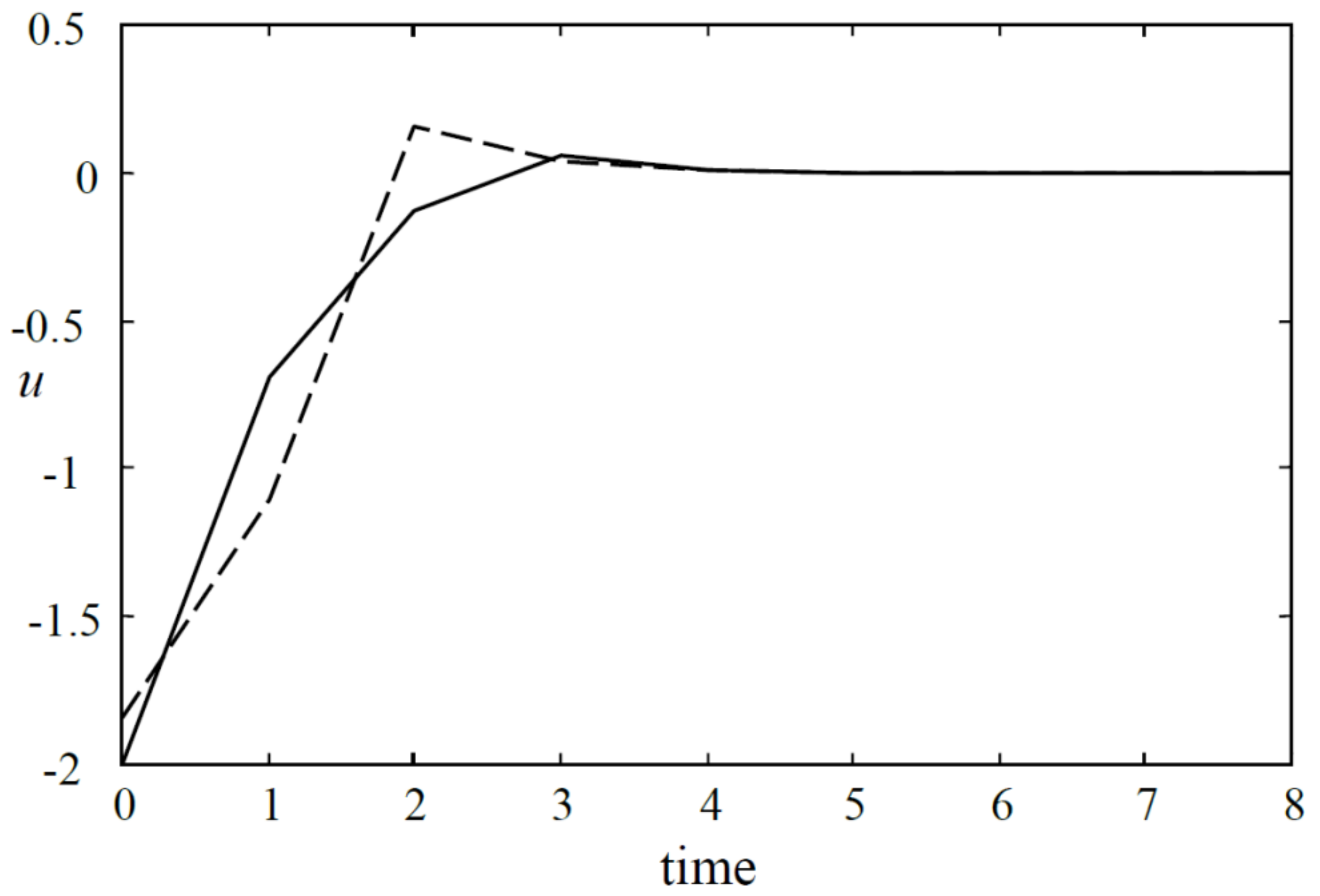
Apply Algorithms 1 and 2. The state and input responses for these two algorithms are shown in Figure 1 and Figure 2, respectively. The upper bounds of the cost value for these two algorithms are and , respectively. Moreover, denote
then for Algorithm 1 and for Algorithm 2. The simulation results show that Algorithm 2 achieves better control performance.
Case 2. Increase . Algorithm 1 becomes infeasible at . However, Algorithm 2 is still feasible by choosing , , , , , , , etc.
4.2. Example 2
Directly consider the system in [9]:
,
where is an uncertain parameter. Use to form a polytopic description and use to calculate the state evolution. The constraints are , , . Choose the weighting matrices as and .
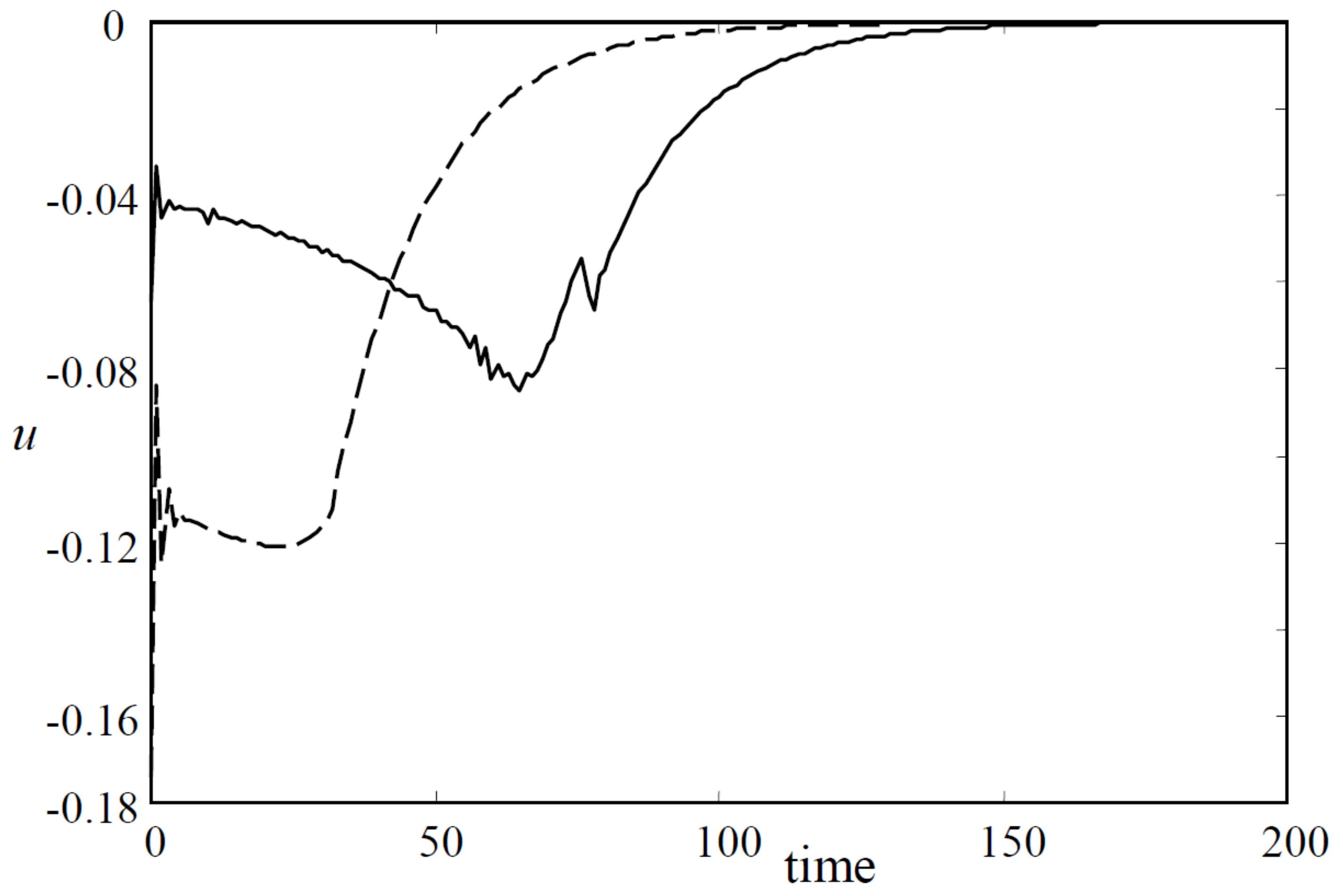
Case 1. Choose and . The initial state lies at . Apply Algorithms 1 and 3. The state trajectories, the state responses and the input responses for these two algorithms are shown in Figure 3, Figure 4 and Figure 5, respectively. Moreover, denote , then for Algorithm 1 and for Algorithm 3.
Case 2. Choose , such that the optimization problem is infeasible for . Then, for Algorithm 1, is , and for Algorithm 3, .
5. Conclusions
In this paper, we have given a new algorithm for off-line robust MPC. The off-line state feedback law is optimized instead, such that each single state feedback law is fixed by the infinite-horizon control moves. This new algorithm consists of MPC with a varying horizon, i.e., the control horizon (say ) varies from M > 1 to M = 1, while the original Algorithm 1 can be taken as an approach with M = 1. Simulation results show that the new algorithm achieves better control performance. Our future research on this topic will be extending it to the output feedback MPC approaches.
Author Contributions
Conceptualization, X.M.; Methodology, X.M.; Software, X.M. and H.B.; Validation, X.M., H.B. and N.Z.; Formal Analysis, X.M.; Investigation, H.B. and N.Z.; Resources, H.B.; Data Curation, X.M. and N.Z.; Writing-Original Draft Preparation, X.M.; Writing-Review & Editing, X.M. and H.B.; Visualization, H.B.; Supervision, X.M.; Project Administration, X.M.
Funding
This research received no external funding.
Acknowledgments
The authors would like to thank Baocang Ding in answering some questions.
Conflicts of Interest
The authors declare no conflict of interest.
References
- Bemporad, A.; Morari, M.; Dua, V.; Pistikopoulos, E.N. The explicit linear quadratic regulator for constrained systems. Automatica 2002, 38, 3–20. [Google Scholar] [CrossRef]
- Mayne, D.Q.; Rawlings, J.B.; Rao, C.V.; Scokaert, P.O.M. Constrained model predictive control: Stability and optimality. Automatica 2000, 36, 789–814. [Google Scholar] [CrossRef]
- Gao, Y.; Dai, L.; Xia, Y.; Liu, Y. Distributed model predictive control for consensus of nonlinear second-order multi-agent systems. Int. J. Robust Nonlinear Control 2017, 27, 830–842. [Google Scholar] [CrossRef]
- Gao, Y.; Xia, Y.; Dai, L. Cooperative distributed model predictive control of multiple coupled linear systems. IET Control Theory Appl. 2015, 9, 2561–2567. [Google Scholar] [CrossRef]
- Bemporad, A.; Morari, M. Robust model predictive control: A. survey. Robustness Ident. Control 1999, 245, 207–246. [Google Scholar]
- Kothare, M.V.; Balakrishnan, V.; Morari, M. Robust constrained model predictive control using linear matrix inequalities. Automatica 1996, 32, 1361–1379. [Google Scholar] [CrossRef] [Green Version]
- Kothare, M.V.; Balakrishnan, V.; Morari, M. Efficient robust predictive control. IEEE Trans. Autom. Control 2000, 45, 1545–1549. [Google Scholar]
- Wan, Z.; Kothare, M.V. Efficient robust constrained model predictive with a time varying terminal constraint set. Syst. Control Lett. 2003, 48, 375–383. [Google Scholar] [CrossRef]
- Wan, Z.; Kothare, M.V. An efficient off-line formulation of robust model predictive control using linear matrix inequalities. Automatica 2003, 39, 837–846. [Google Scholar] [CrossRef]
- Li, D.; Xi, Y.; Zheng, P. Constrained robust feedback model predictive control for uncertain systems with polytopic description. Int. J. Control 2009, 82, 1267–1274. [Google Scholar] [CrossRef]
- Garone, E.; Casavola, A. Receding horizon control strategies for constrained LPV systems based on a class of nonlinearly parameterized Lyapunov functions. IEEE Trans. Autom. Control 2012, 57, 2354–2360. [Google Scholar] [CrossRef]
- Huang, H.; Li, D.; Lin, Z.; Xi, Y. An improved robust model predictive control design in the presence of actuator saturation. Automatica 2011, 47, 861–864. [Google Scholar] [CrossRef]
- Shi, T.; Su, H.; Chu, J. An improved model predictive control for uncertain systems with input saturation. J. Franklin Inst. 2013, 350, 2757–2768. [Google Scholar] [CrossRef]
- Chisci, L.; Zappa, G. Feasibility in predictive control of constrained linear systems: The output feedback case. Int. J. Robust Nonlinear Control 2002, 12, 465–487. [Google Scholar] [CrossRef]
- Ding, B.; Pan, H. Output feedback robust MPC for LPV system with polytopic model parametric uncertainty and bounded disturbance. Int. J. Control 2016, 89, 1554–1571. [Google Scholar] [CrossRef]
- Ping, X.; Ding, B. Off-line approach to dynamic output feedback robust model predictive control. Syst. Control Lett. 2013, 62, 1038–1048. [Google Scholar] [CrossRef]
- Ding, B.; Xi, Y.; Li, S. A synthesis approach of on-line constrained robust model predictive control. Automatica 2004, 40, 163–167. [Google Scholar] [CrossRef]
- Ding, B.; Xi, Y.; Cychowski, M.T.; O’Mahony, T. Improving off-line approach to robust MPC based-on nominal performance cost. Automatica 2007, 43, 158–163. [Google Scholar] [CrossRef]
Figure 1.
The state responses of the closed-loop systems (dashed line for Algorithm 1, solid Algorithm 2).
Figure 1.
The state responses of the closed-loop systems (dashed line for Algorithm 1, solid Algorithm 2).
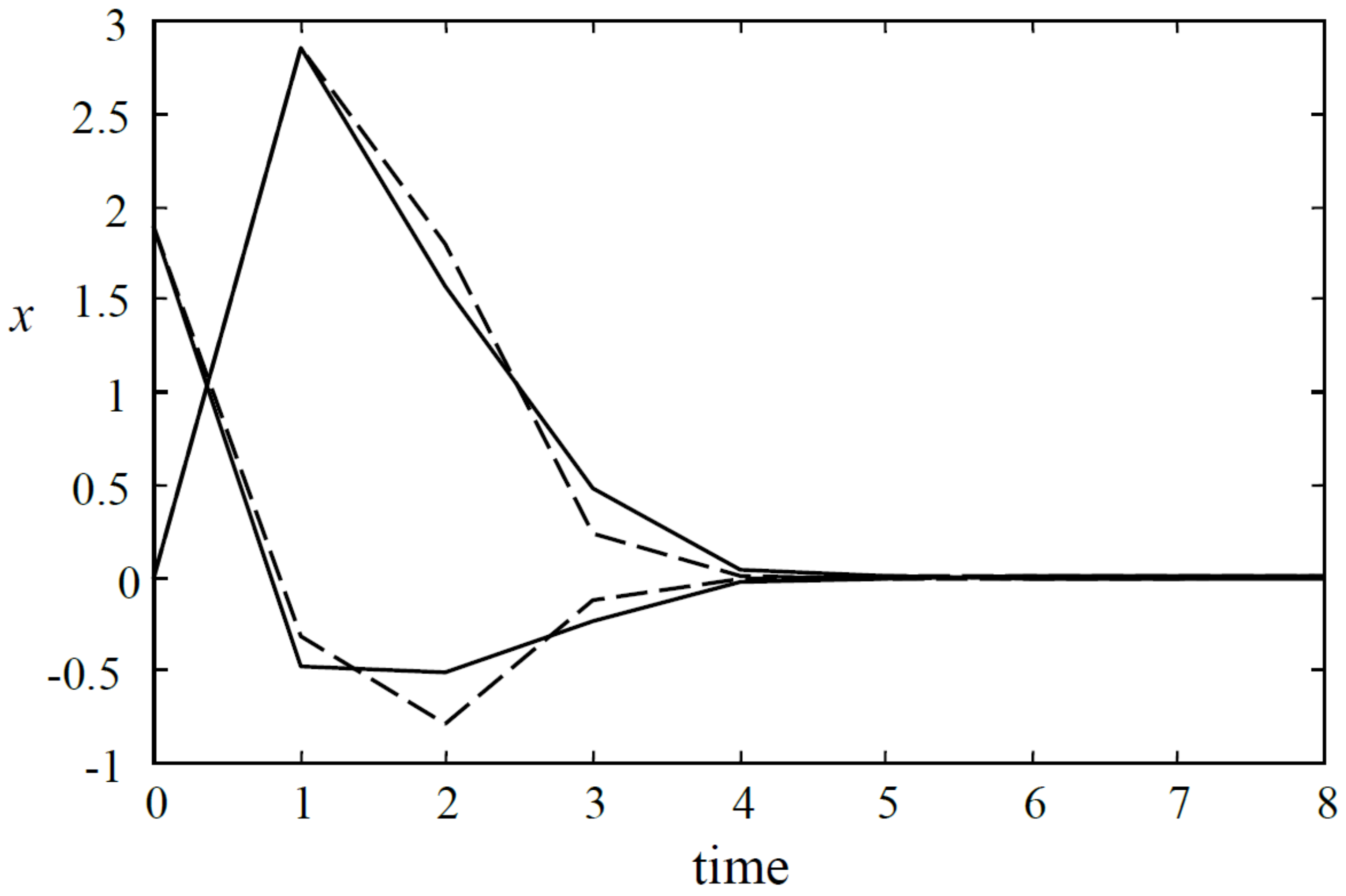
Figure 2.
The input responses of the closed-loop system (dashed line for Algorithm 1, solid Algorithm 2).
Figure 2.
The input responses of the closed-loop system (dashed line for Algorithm 1, solid Algorithm 2).

Figure 3.
The state trajectories of the closed-loop systems (dashed line for Algorithm 1, solid Algorithm 3).
Figure 3.
The state trajectories of the closed-loop systems (dashed line for Algorithm 1, solid Algorithm 3).
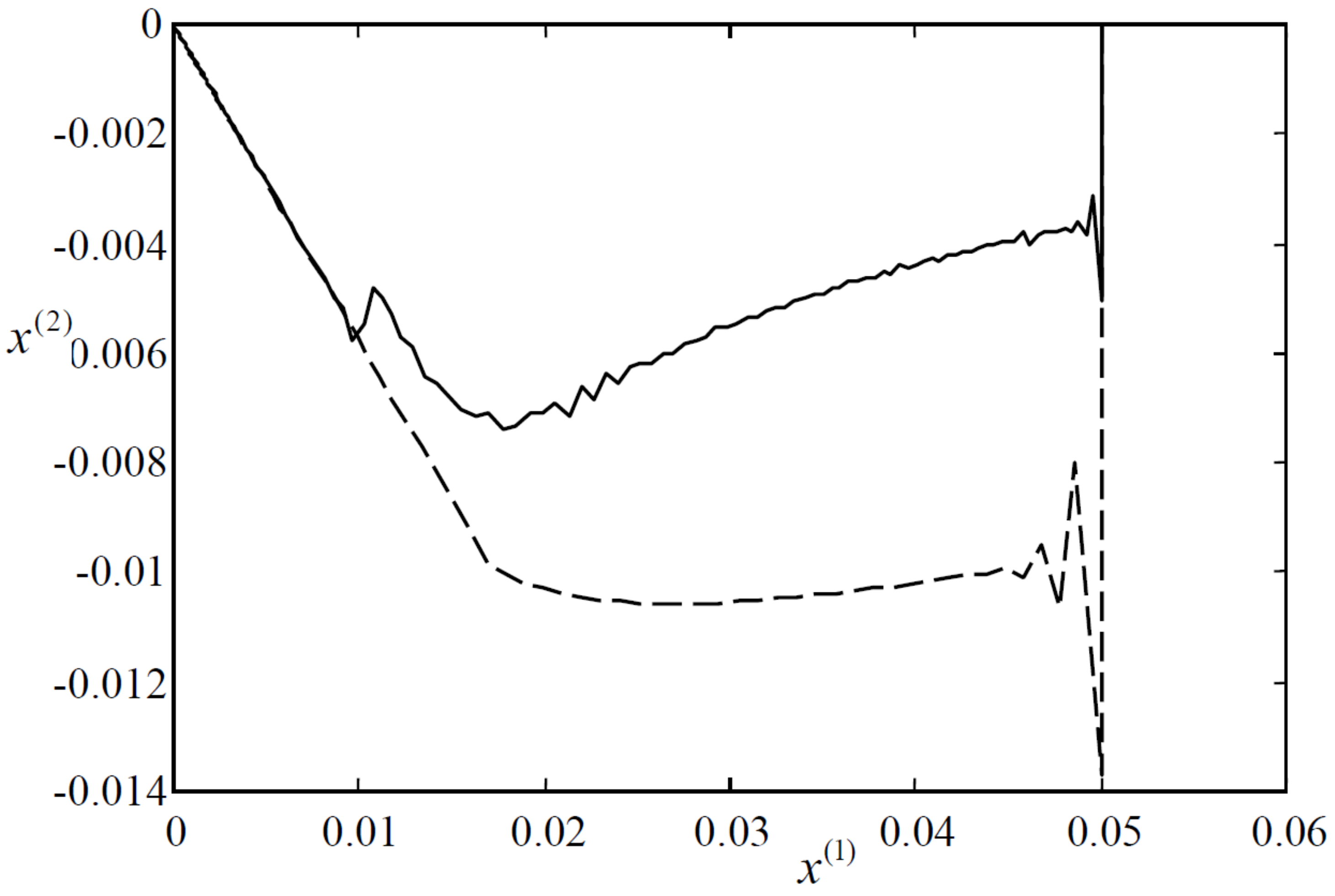
Figure 4.
The state responses of the closed-loop systems (dashed line for Algorithm 1, solid Algorithm 3).
Figure 4.
The state responses of the closed-loop systems (dashed line for Algorithm 1, solid Algorithm 3).

Figure 5.
The input responses of the closed-loop systems (dashed line for Algorithm 1, solid Algorithm 3).
Figure 5.
The input responses of the closed-loop systems (dashed line for Algorithm 1, solid Algorithm 3).

© 2018 by the authors. Licensee MDPI, Basel, Switzerland. This article is an open access article distributed under the terms and conditions of the Creative Commons Attribution (CC BY) license (http://creativecommons.org/licenses/by/4.0/).
Share and Cite
MDPI and ACS Style
Ma, X.; Bao, H.; Zhang, N. A New Approach to Off-Line Robust Model Predictive Control for Polytopic Uncertain Models. Designs 2018, 2, 31. https://doi.org/10.3390/designs2030031
AMA Style
Ma X, Bao H, Zhang N. A New Approach to Off-Line Robust Model Predictive Control for Polytopic Uncertain Models. Designs. 2018; 2(3):31. https://doi.org/10.3390/designs2030031
Chicago/Turabian StyleMa, Xianghua, Hanqiu Bao, and Ning Zhang. 2018. "A New Approach to Off-Line Robust Model Predictive Control for Polytopic Uncertain Models" Designs 2, no. 3: 31. https://doi.org/10.3390/designs2030031