Navigation of an Autonomous Wheeled Robot in Unknown Environments Based on Evolutionary Fuzzy Control

Abstract

Navigation of a wheeled robot in unknown environments is proposed in this paper. The approach may be applied to navigating an autonomous vehicle in unknown environments, such as parking lots. The navigation consists of three parts: obstacle avoidance behavior, target seeking behavior, and a behavior supervisor. The obstacle avoidance behavior is achieved by controlling the robot to move along an obstacle boundary through evolutionary fuzzy control. In the evolutionary fuzzy control approach, a Pareto set of fuzzy controllers (FCs) is found though a multi-objective continuous ant colony optimization algorithm. Target seeking behavior is achieved by controlling the robot through hybrid proportional–integral–derivative (PID) controllers. The behavior supervisor determines the switching between obstacle avoidance and target seeking behaviors, where the dead-cycle problem is considered. Simulations and experiments were performed to verify the effectiveness of the proposed navigation scheme.

1. Introduction

Navigation is an important task for autonomous vehicles and robots. Localization is an important function in navigation. The sensors generally used in the positioning system of autonomous vehicles include Global Positioning Systems (GPS), inertial measurement units, Light Detection and Ranging (LIDAR), and camera sensors [1,2]. When lane markings are available, lane-detection systems, based on LIDAR [3], and/or cameras [4,5], can provide lateral distance measurements from the lane markings to the vehicle for lane-level navigation [6]. When load maps that contain accurate geometry of all lanes and the three-dimensional (3D) structure of roads, such as overpasses, are known in advance, navigation accuracy can be improved [7]. In unknown environments without lane markings, such as basements and suburbs, another navigation approach needs to be developed. The techniques of robot navigation in unknown environments may be employed to address this problem.

This paper considers the navigation of a wheeled robot in unknown environments. One important task in navigating a car [8] or a robot [9,10,11,12,13,14] is obstacle avoidance. To complete this task, fuzzy control of mobile robots and car-like robots has been proposed [9,10,11,12,13,14]. The reason why fuzzy controllers (FCs) have been extensively used in this application is because their generic characteristics can handle complicated topographies. The parameters in the FCs employed in [9,10,11,12] were obtained from manual tuning. This manual design approach is time consuming and the performance of the designed FC may be unsatisfactory because it is hard to find an optimal parameter set through hand crafting. In addition, for the obstacle avoidance approach in [10,11], the FC used contains only two (left and right) sensors, which is too simple to avoid collisions with obstacles of different shapes in complex maps. The collision-free approach in [12] uses the width of the obstacle to generate the coordinate as a temporary target to avoid collision with obstacles. However, this method would not work properly in some situations, such as when an obstacle is too large for a laser sensor to detect its boundary.

To address the above problems, evolutionary learning of FCs for obstacle avoidance through different swarm intelligence algorithms has been proposed [13,14,15]. In this approach, when a robot meets an obstacle, it is controlled to move along the obstacle boundary to avoid collisions. Different algorithms towards optimizing the parameters in an FC have been proposed, including discrete ant colony optimization (ACO) [13] and evolutionary group-based particle swarm optimization (EGPSO) [14], to name just a few. The FCs used in these methods only consider robot–obstacle distance, with the robot moving at a constant speed. Multi-objective optimization of an FC that optimizes robot–obstacle distance, moving speed, and rule interpretability has been proposed [15]. Given the three objectives, the multi-objective front-guided continuous ant-colony optimization (MO-FCACO) algorithm was proposed to optimize FCs. In this approach, rules are generated using a clustering algorithm, where the number of rules is equal to the number of clusters. The designed FC is applied to control a robot for wall following. This paper applies the MO-FCACO to optimize FCs for obstacle boundary following (OBF) in a navigation task. The OBF behavior ensures a collision-free behavior and enables the robot to bypass obstacles. To simplify the design task, this paper focuses on the two objectives of optimizing robot–obstacle distance and moving speed. The number of rules in the optimized FCs is assigned in advance; the interpretability of the FCs is disregarded. Different from [15], a new objective function, measuring the performance of the robot–obstacle distance is proposed. This modification is proposed to improve the control performance when the robot turns around the corner of an obstacle.

Navigation of a mobile robot can be divided into navigation in known and unknown environments. For navigation in known environments, the environment map is available in advance. The task of navigation aims to find an optimal robot path in the given map. One popular approach is the A* algorithm [16] and its variants [17,18,19]. This paper considers navigation in unknown environments. Different navigation approaches in unknown environments have been proposed [14,20,21,22,23,24,25,26]. Among them, one efficient navigation approach that avoids the dead-cycle problem was proposed in [14]. The dead-cycle problem means that a robot moves around in circles or cycles between multiple traps. Based on the navigation approach in [14], this paper proposes the following improvements. The first improvement concerns the locomotion control. The robot moves at a constant speed when it executes the OBF and target searching (TS) behaviors in [14]. In addition, the robot has to stop and rotate at the same site when it switches from the OBF to TS behavior. In this paper, FC and hybrid proportional-integral-derivative (PID) controllers are proposed to control the robot in executing the OBF and TS behaviors, respectively. Both the orientation and speed of the robot are controlled in executing each behavior and the robot smoothly switches from the OBF to TS behavior without stopping. The second improvement concerns the sensing and localization. To improve the accuracy of robot–obstacle distance measurement, the sonar sensors in [14] are replaced by a laser sensor in this paper. Based on the sonar sensor measurements, the robot is controlled, to move within the robot–obstacle distance range of [0.1, 1] m in executing the OBF in [14]. In this paper, the robot is controlled, to main a constant robot–obstacle distance of 0.5 m, based on the laser sensor measurements. Regarding the localization, the rotary encoders equipped in the robot are used for localization in [14]. In this paper, the robot is mainly localized using the hybrid of a Stargazer sensor (http://www.hagisonic.com) [27] and the rotary encoders. The experimental results obtained from the navigation of a Pioneer 3-DX robot verify the effectiveness of the proposed method.

This paper is organized as follows: Section 2 describes the rules in the FC and the two objective functions defined to optimize FCs in executing the OBF behavior. This section also describes the MO-FCACO used to optimize the FCs and introduces the proposed navigation scheme, including the hybrid PID controllers for TS. Section 3 presents simulations and experimental results. Finally, Section 4 presents conclusions.

2. Materials and Methods

2.1. Fuzzy Controller and Obstacle Avoidance Behavior

Navigation consists of the two behaviors of TS and obstacle avoidance and a behavior supervisor. In this paper, the obstacle avoidance behavior is achieved by controlling a robot to execute the OBF. This paper employs an FC to control the robot in executing the OBF behavior. This section introduces the used FC and the control objective functions.

2.1.1. Fuzzy Controller

Each fuzzy rule in the FC is described as follows:

$$\begin{gathered} R_i:\mathrm{If} x_1\left(k\right) \mathrm{is} A_{i1} \mathrm{And}\dots \mathrm{And} x_n\left(k\right) \mathrm{is} A_{in} \\ {\mathrm{Then} \mathrm{y}}_1\left(\mathrm{k}\right) \mathrm{is} b_{i1} \mathrm{And}\dots \mathrm{And} y_m\left(k\right) \mathrm{is} b_{im} \end{gathered}$$

(1)

where $x_1\left(k\right),\dots ,x_n\left(k\right)$ are distance sensor inputs, $y_1\left(k\right),\dots ,y_m\left(k\right)$ are output control variables, $b_{i1},\dots ,b_{im}$ are real numbers, and $A_{i1},\dots ,A_{in}$ are fuzzy sets. By using the algebraic product for fuzzy-AND operation and the weighted-average defuzzifier, the output of the FC is calculated by

$$y_m\left(k\right)=\frac{{\sum }_{i=1}^r{\prod }_{j=1}^n{\mu }_{ij}\left(x_j\right)b_{im}}{{\sum }_{i=1}^r{\prod }_{j=1}^n{\mu }_{ij}\left(x_j\right)}$$

(2)

where $r$ is the number of rules and ${\mu }_{ij}$ is a Gaussian membership function of $A_{ij}$ and is given by

$${\mu }_{ij}\left(x_j\right)=exp\left\{-{\left(\frac{x_j-m_{ij}}{{\sigma }_{ij}}\right)}^2\right\}$$

(3)

where $m_{ij}$ is the center and ${\sigma }_{ij}$ is the width of the fuzzy set $A_{ij}$. In the design of the FC, manual selection of the FC parameters to execute the OBF behavior is time consuming. Therefore, all the free parameters in the FC are learned through an evolutionary FC approach. The parameters to be optimized include the center $m_{ij}$ and width ${\sigma }_{ij}$ of each fuzzy set in the antecedent part and $b_{im}$ in the consequent part. Therefore, given a pre-assigned number of rules $r$, the parameter solution vector $\stackrel{\rightharpoonup }{s}$ in an FC can be represented by

$$\begin{gathered} \stackrel{\rightharpoonup }{s}=[m_{11},{\sigma }_{11},\dots ,m_{1n},{\sigma }_{in},b_{11},\dots ,b_{1m},\dots \\ \dots ,m_{r1},{\sigma }_{r1},\dots ,m_{rn},{\sigma }_{rn},b_{r1},\dots ,b_{rm}]\in {\Re }^{r(2n+m)} \end{gathered}$$

(4)

2.1.2. Multiple Control Objectives

Navigation of a wheeled Pioneer 3-DX robot is considered. This robot includes two wheels and one caster. A laser rangefinder is used as a distance sensor. The scanning range of the right-side is divided into four ranges: $\left[0°,25°\right]$, $\left[25°,45°\right]$, $\left[45°,70°\right]$, and $\left[70°,90°\right]$. The minimum reading from each range is denoted as $x_i$, $i$ = 1, …, 4. For the right OBF, the four readings from the right side are fed as FC inputs, i.e., $n$ = 4 in Equation (1). The FC sends two outputs to control the speeds of the left and right wheels, i.e., m = 2 in Equation (1). Figure 1 shows the training map in the evolutionary FC approach. The FC is designed to control the robot with the two objectives of maintaining a proper robot–obstacle distance and moving along the obstacle boundary with a fast-moving speed. The two control objective functions are evaluated over a maximum number of $T_{total}$ (=1500) control time steps and are defined, as follows.

The first objective function $f_1$ is given by

$$f_1=\frac{{\sum }_{t=1}^{T_s}\left|\frac{L_{wall}\left(t\right)}{d_{wall}+d_{bou}}-1\right|+10\times P_e}{T_S}+(T_{toal}-T_S)$$

(5)

where $L_{wall}\left(t\right)$ is the sensor measurement at nearly $90°$, $d_{wall}$ (=0.5 m) is the desired distance from the robot’s right-side boundary to the obstacle, and $d_{bou}$ (=0.2 m) is the distance from the laser to the robot’s right-side boundary. The time step, $T_s$, is the total number of control time steps before control fails. An FC is deemed as failed if the robot is far away from the obstacle ($x_3$ or $x_4$ > 2 m) for two consecutive steps or too close to the obstacle ($\underset{i}{\min }{x}_i$ < 0.3 m). The number of uncompleted steps $T_{total}-T_S$ is used as a penalty in Equation (5) for a failed control. Different from [15], an additional term $P_e$ is included in this objective function, to avoid a large deviation from the desired distance when the robot is turning around a corner. The initial value of $P_e$ is set to zero and is accumulated by one if a large deviation occurs, i.e.,

$$P_e\left(t+1\right)=\{\begin{array}{cc}{P}_e\left(t\right)+1,& \mathrm{if} |x_4-(d_{wall}+d_{bou})|>0.3 m\\ P_e\left(t\right),& \mathrm{otherwise}\end{array}$$

(6)

The second objective function, $f_2$, is given by

$$f_2=\frac{1}{{\sum }_{t=1}^{T_s}\left|\frac{V_{speed}\left(t\right)}{T_s}\right|}+(T_{toal}-T_S)$$

(7)

where $V_{speed}\left(t\right)$ is the speed of the robot. The aim of this objective function is to control the robot to move as quickly as possible.

To maintain a constant distance from the obstacle, the robot should move with a low speed. Because of the trade-off between these two objectives, the control problem can be formulated as a multi-objective optimization problem. Instead of converting the multi-objective optimization problem to a single-objective optimization problem and finding only a single FC solution, this paper applies a multi-objective optimization algorithm to find a Pareto set of FC solutions. The MO-FCACO [15] was used to address this control problem. The MO-FCACO was originally proposed to optimize interpretable FCs. This paper applies the MO-FCACO to optimize FCs with the only consideration being control performance. The next section describes the MO-FCACO.

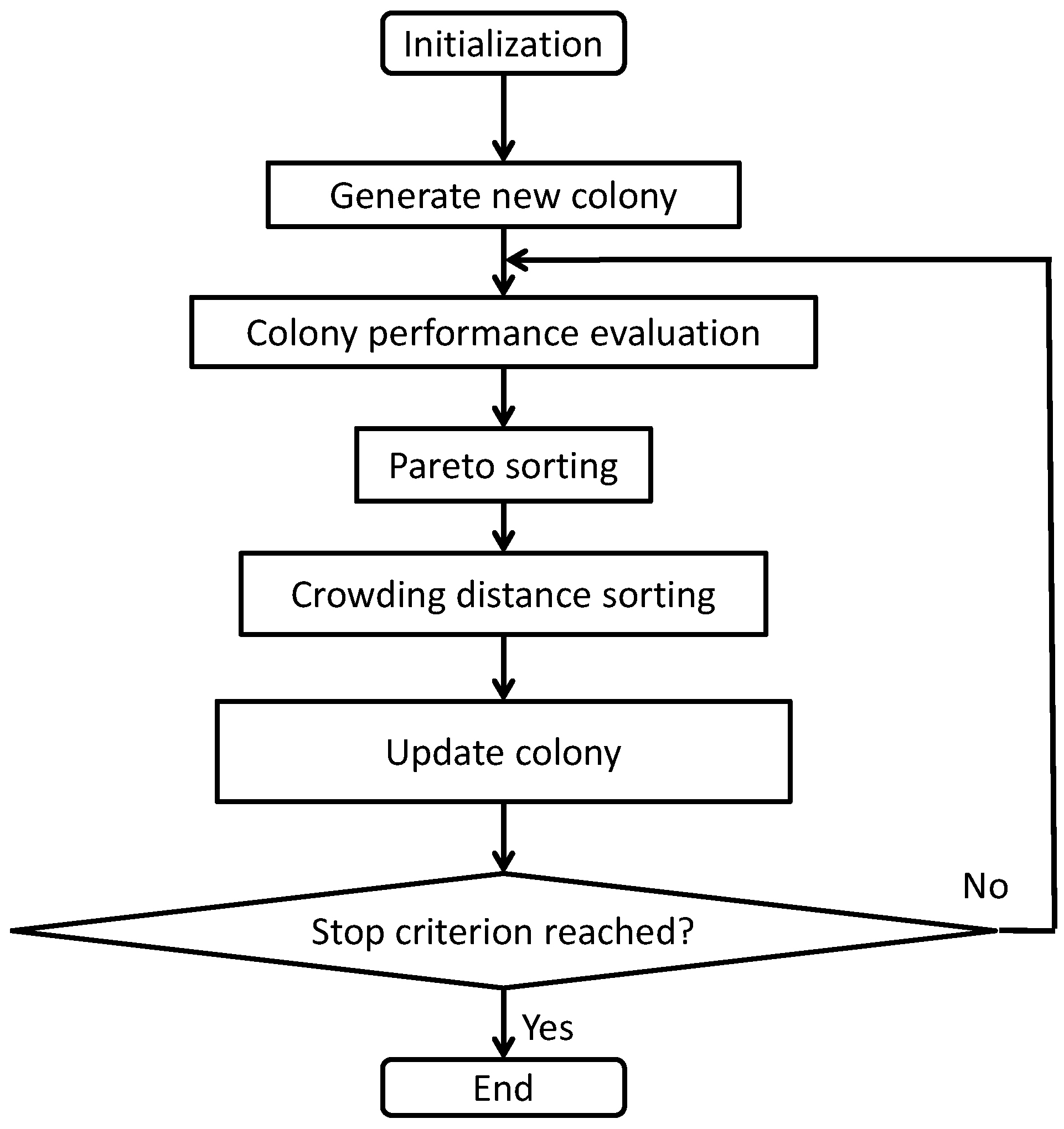
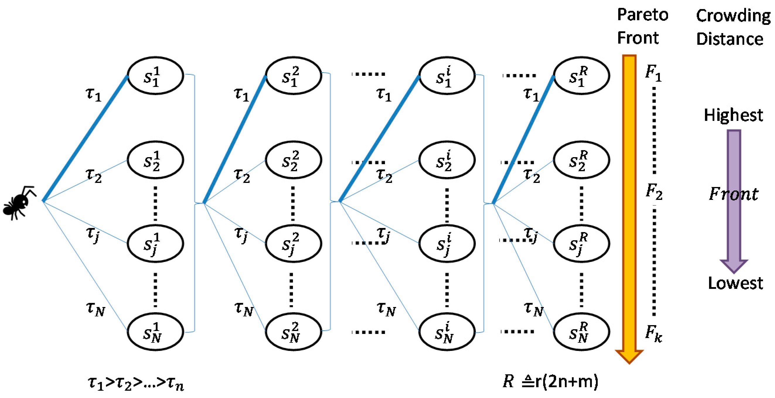
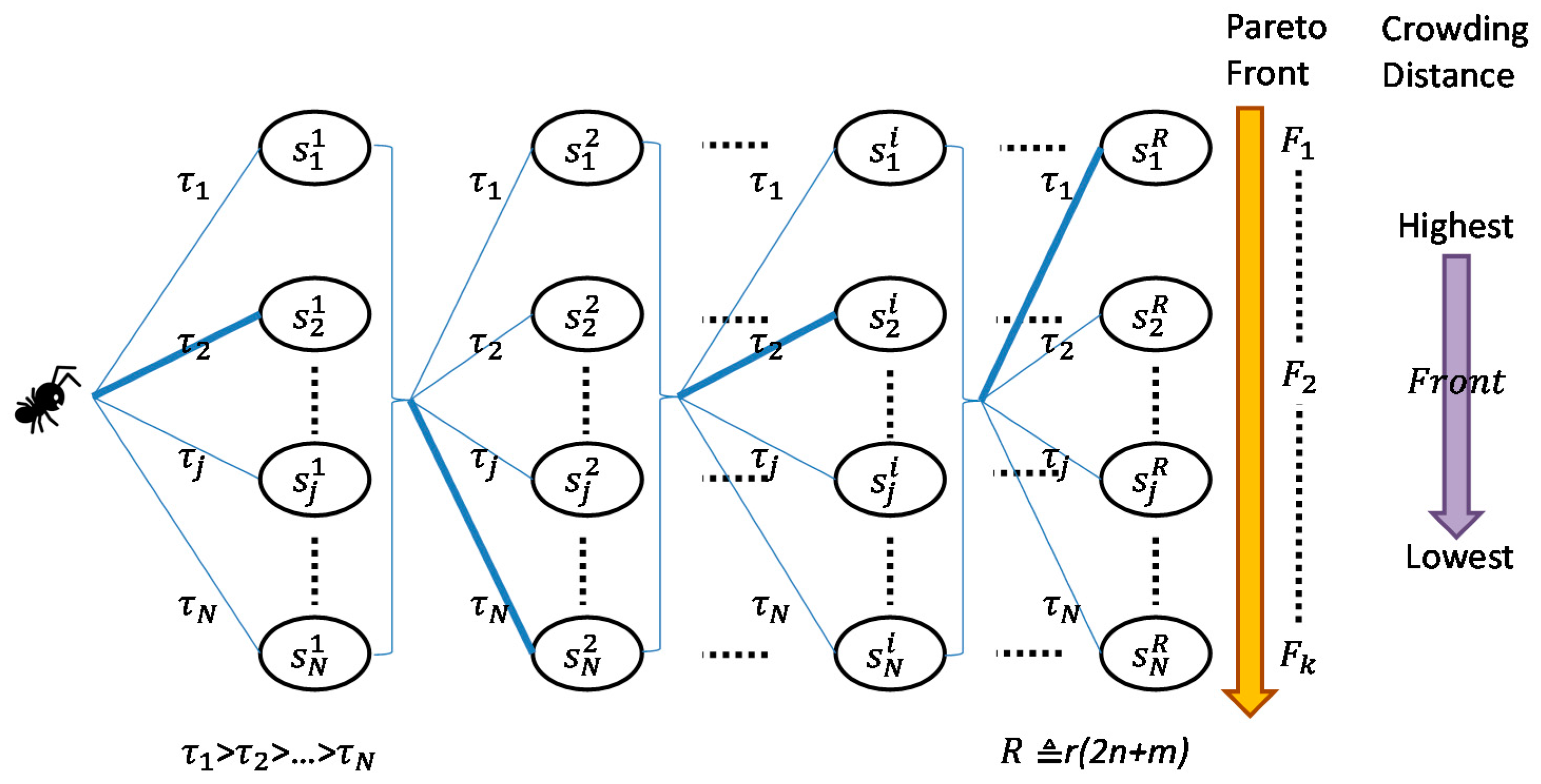
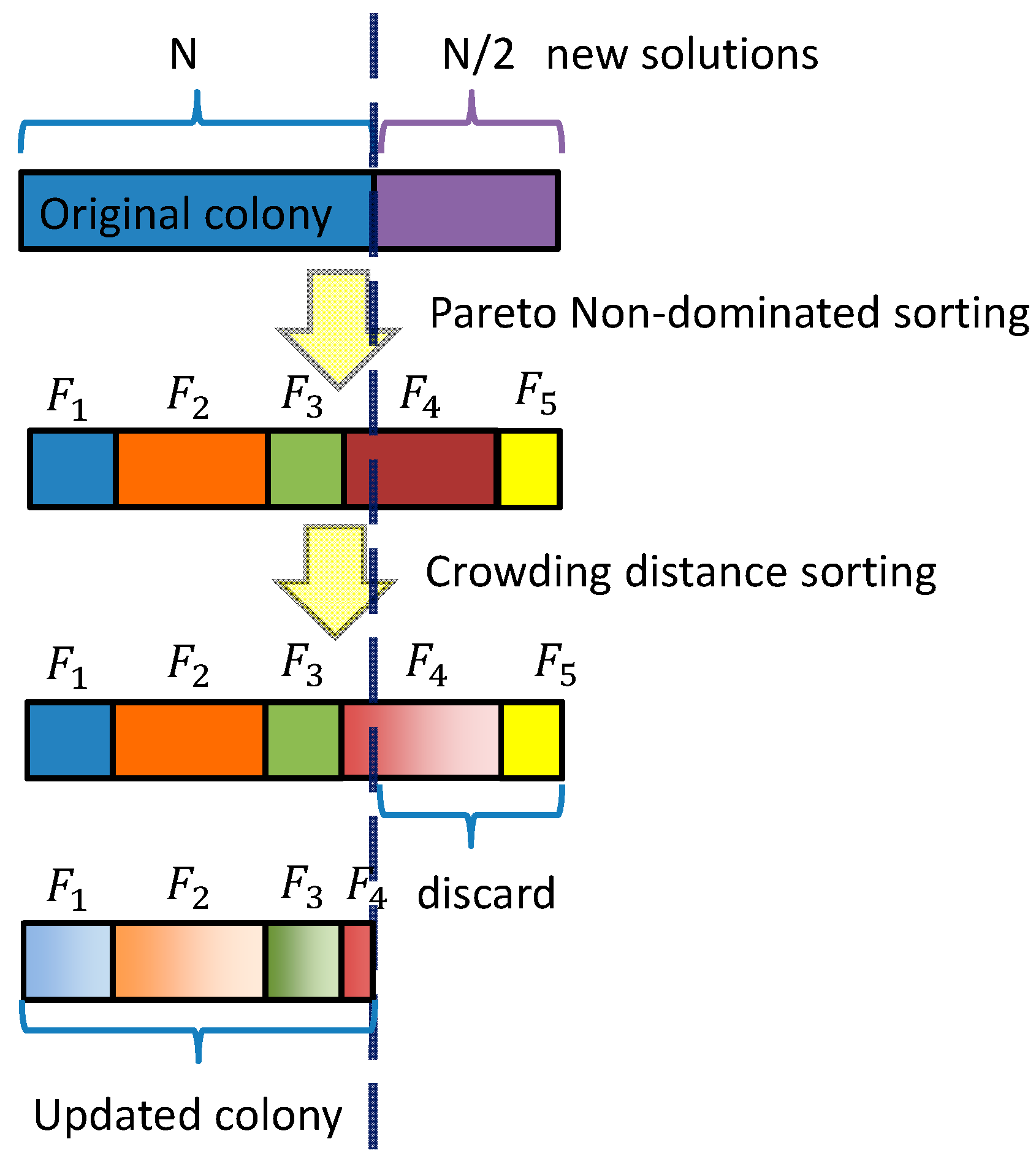
2.2. Multi-Objective Front-Guided Continuous Ant Colony Optimization

Figure 2 shows the flowchart of the MO-FCACO. A population contains a colony of ants. Each ant selects a parameter solution vector ${\stackrel{\rightharpoonup }{s}}_i$ of an FC, as shown in Equation (4). The length of a solution vector depends on the number of input sensor readings, $n$, the number of FC outputs, $m$, and the number of fuzzy rules, $r$. The population size is denoted as N. The jth component in solution ${\stackrel{\rightharpoonup }{s}}_i$ is denoted as $s_i^j$. The initial population of solutions is randomly generated. After evaluation of the N initial solutions, by applying their decoded FCs to control the robot in the training environment, the solutions are sorted according their objective function values. The non-dominated sorting approach [28] is used. In the non-dominated sorting, the non-dominated solutions constitute the first front $F_1$. Solutions in front $F_l$ are dominated only by those in $F_1$ to $F_{l-1}$. For solutions in the same front, performances are sorted according to their crowding distances, to maintain solution diversity.

Figure 3 shows a graphical representation of the solution generation scheme, in terms of nodes and path segments. Each node represents a solution component. Each path segment is associated with a pheromone level, where a higher pheromone level is assigned to the path segments connecting to the nodes in a better performed solution vector. The solutions are sorted from the best to the worst, so ${\tau }_1>{\tau }_2>\dots >{\tau }_N$. For a new iteration, N/2 new solutions are generated from N/2 ant selected paths. Half of the new solutions are generated from elite selection and the other half from tournament selection. In the elite selection, the original solutions with higher pheromone levels are selected, as shown in Figure 3. Therefore, the best one quarter of current N solutions are selected. In the tournament selection, an ant randomly and uniformly selects two path segments and the one with a larger pheromone level is selected, as shown in Figure 4. The node connected to the selected path segment constitutes a solution component.

After generating the N/2 temporary solutions, a Gaussian sampling operation is applied to all solution components. For a solution component $s_i^j$ in the temporary solution, the mean $c_i^j$ of the Gaussian probability density function is set to be $s_i^j$. The standard deviation (SD) ${\sigma }_i^j$ of the Gaussian operation is computed, based on the other $N-1$ possible solution components of variable $j$ and is calculated by

$${\sigma }_i^j=\epsilon \times {\displaystyle \sum }_{l=1,l\ne i}^N\frac{\left|c_i^j-s_l^j\right|}{N-1}$$

(8)

The constant $\epsilon$ affects the spread of new solutions after this operation and is set to 0.85. Finally, these new temporary solution vectors ${\widetilde{\stackrel{\rightharpoonup }{s}}}_i$ move toward a well-performed solution ${\stackrel{\rightharpoonup }{s}}_{i^{\ast }}$, randomly selected from front 1. The new solutions are

$$s_{N+i}^j={\tilde{s}}_i^j+\phi ·(s_{i^{\ast }}^j-{\tilde{s}}_i^j)i=1,\dots ,N/2$$

(9)

where $\phi$ is a uniformly distributed random number in [0, 1].

The N/2 new solutions function as N/2 new FCs and are applied to the robot in the training map to obtain the two objective function values. After the performance evaluation process, the N/2 new solutions and the original N solutions in the population are sorted again, based on the Pareto non-dominated sorting and crowding distances. Finally, only the best N solutions are reserved, as shown in Figure 5. The new solution generation, performance evaluation, and performance sorting, and solution elimination operations are repeated until the stopping condition of a maximum number of iterations is reached.

2.3. Navigation

This section introduces the use of the TS control, followed by the behavior supervisor (BS), to navigate the robot in unknown environments. The TS control uses hybrid PID controllers to control the orientation and moving speed of the robot in reaching the target. The BS determines switching between the TS and OBF behaviors.

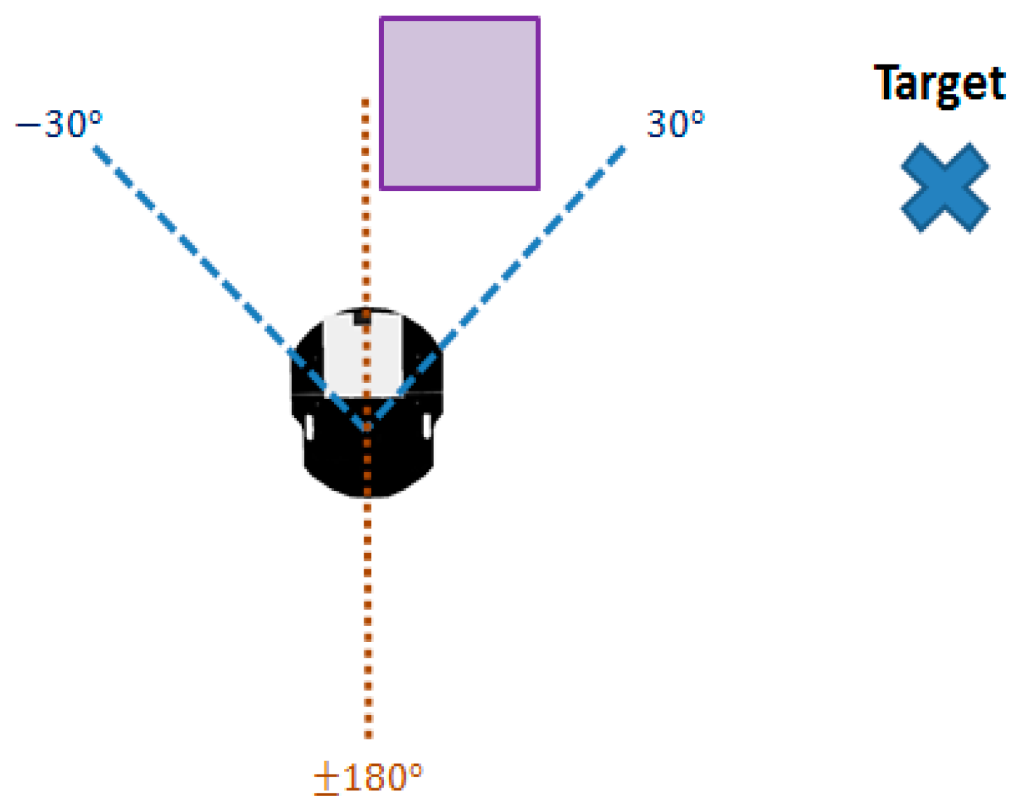
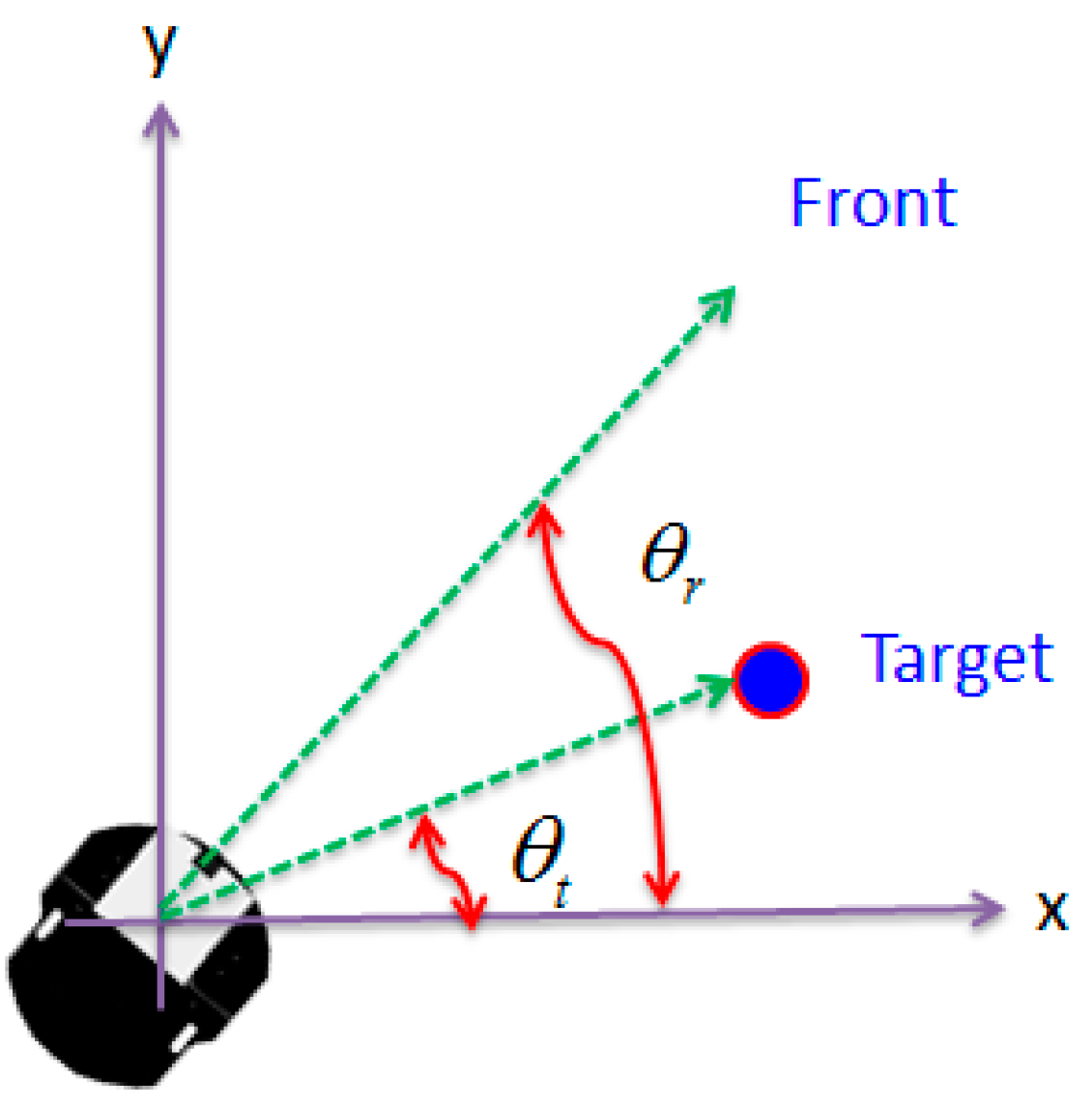
2.3.1. Target Seeking

Moving toward a target is the most important task in navigating a robot. Therefore, the first step in TS is determining the deviation angle between the robot front direction and a target. The positions of the target and the robot are recorded using the world coordinate. The position and orientation of the robot are obtained from a localization system. Figure 6 shows the angle ${\theta }_r$ of the front direction of the robot and the angle ${\theta }_t$ of the target. The angle devigation ${\theta }_{TS}$ $\in \left[-{180}^0,{180}^0\right]$ between the robot and the target is calculated by

$${\theta }_{TS} ={\theta }_t-{\theta }_r$$

(10)

In the hybrid PID control approach, two PID controllers, named the velocity-PID controller and the orientation-scheduled PID controller are designed to control the robot moving speed and orientation when reaching a target, respectively.

The velocity-PID controller outputs $V_{basic}\left(t\right)$ control the common speed of the left and right wheels. The control error is defined to be the distance $D_T \left(t\right)$ between the robot and the target. The velocity-PID controller is represented by

$$V_{basic}\left(t\right)=K_{P1}{D}_T\left(t\right)+K_{I1}{\displaystyle \sum }_{k=1}^t{D}_T\left(k\right)·\Delta t+K_{D1}\left[D_T\left(t\right)-D_T\left(t-1\right)\right]/\Delta t$$

(11)

where $\Delta t$ is the time between measurements of $D_T$. The units of $V_{basic}\left(t\right)$, $D_T\left(t\right)$, and $\Delta t$ are rad/s, cm, and sec., respectively. This paper sets $K_{P1}=1/100$, $K_{I1}=1/200$, and $K_{D1}=1/100$. An upper bound of 10 rad/s = 0.98 m/s is imposed on $V_{basic}\left(t\right)$ to avoid saturation, when combined with the orientation controller.

The orientation-PID controller output $V_{ore}\left(t\right)$ controls the velocity of the right wheel. The orientation PID controller is represented by

$$V_{ore}\left(t\right)=K_{P2}{\theta }_{TS}\left(t\right)+ K_{I2}{\displaystyle \sum }_{k=1}^t{\theta }_{TS}\left(k\right)·\Delta t+K_{D2}\left[{\theta }_{TS}\left(t\right)-{\theta }_{TS}\left(t-1\right)\right]/\Delta t$$

(12)

where the units of $V_{ore}\left(t\right)$, ${\theta }_{TS}\left(t\right)$, and $\Delta t$ are rad/s, degree, and sec., respectively.

The output $V_{ore}\left(t\right)$ is added to the original right wheel velocity. Via the combination of the velocity and orientation PID controllers, the final speed control signals sent to the left and right wheels are:

$$\{\begin{array}{c}{V}_{right}\left(t\right)=V_{basic}\left(t\right)+V_{ore}\left(t\right)\\ V_{left}\left(t\right)=V_{basic}\left(t\right)\end{array}$$

(13)

The output $V_{ore}\left(t\right)$ is applied only to the right wheel, rather than to the two wheels in equal and opposite directions, in order to keep the robot at a high moving speed.

In the selection of the PID coefficients in Equation (12), a scheduled coefficient is proposed. For a large deviation ($|{\theta }_{TS}|>{45}^0$), the coefficient set $K_{P2}=1/10$, $K_{I2}=3/200$, and $K_{D2}=1/50$ is selected to reduce rise time. For a smaller deviation ($|{\theta }_{TS}|<{45}^0$), a smaller coefficient set $K_{P2}=1/15$, $K_{I2}=3/400$, and $K_{D2}=1/50$ is selected to reduce overshoot.

2.3.2. Behavior Supervisor

This section introduces the BS that determines the switching between TS and OBF behaviors. First, the surroundings of the robot are divided into three regions, to determine if there are any obstacles in the forward moving direction. The front, right, and left regions lie in $\left[-30°,30°\right]$, [$0°,180°$], and $\left[-180°,0°\right]$, respectively. The robot executes the TS behavior if the robot does not meet an obstacle (i.e., minimum sensor value <0.7 m) in the region at which the target is located. The neighboring regions are overlapped to avoid collision of the robot with an obstacle when the robot executes the TS behavior. Figure 7 shows an example of the reason why the regions are overlapped. If the right region lies in $\left[30°,180°\right]$, where there is no obstacle, the robot executes the TS behavior. With the PID control, the robot cannot turn immediately toward the target while moving forward. The forward movement would cause the robot to collide with the obstacle in front. The divided regions and control strategy are different from those in [14], where the left and right regions do not overlap the front region. In [14], to execute the TS, the robot first stops and rotates on site to the direction of the target, after which the robot moves directly toward the target. The proposed control method does not stop the robot, which reduces the time taken to reach a target.

The robot switches to the OBF behavior when it meets an obstacle in the direction of the target. The choice between the right or left OBF is determined by the minimum laser sensor measurements. If the minimum measurement belongs to the left (right)-half region, then the robot executes the left (right) OBF. Though the robot only learns the right OBF behavior in Section 3, the left OBF behavior is directly available due to symmetric properties.

To avoid the dead-cycle problem, the BS in [14] is used with some modifications. In this BS, when the robot switches from TS to OBF, the distance from the robot to the target is stored in $d_1$. If the behavior changes from OBF to TS, the current robot–target distance $d_2$ should be less than $d_1$. This mechanism ensures that the robot gets closer to the target through the TS behavior and remedies the dead-cycle problem. Another switch variable, the step counter $C_{step}$, is also considered in the behavior switching process, to avoid oscillations due to fast behavior changes, especially in real experiments. Different from the BS in [14], an additional condition, allowing the switching from OBF to TS is considered. That is, if the robot–target distance is smaller than the laser sensing range and no obstacle is found in the target regions, then the robot switches from OBF to TS. This additional switching condition reduces path length, as shown in Figure 8. The switching condition was not used in [14] because of the usage of low sensing range of the sonar sensors. It should be noted that the objective in Figure 8 is to show the difference of the BS between [14] and the proposed method. Therefore, the same FC designed using the MO-FCACO for OBF was used to control the robot in Figure 8.

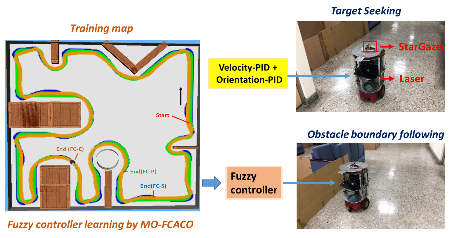
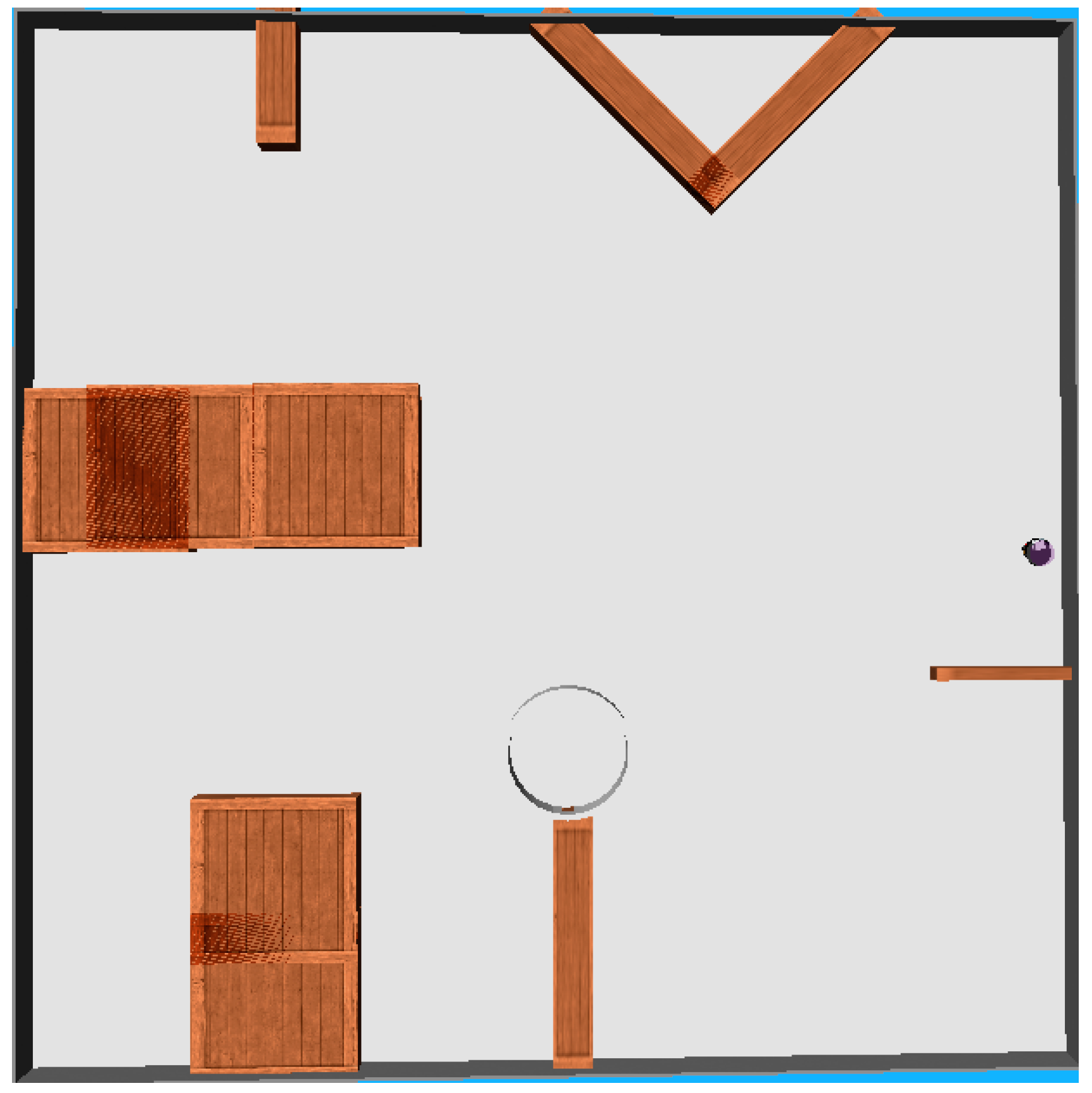
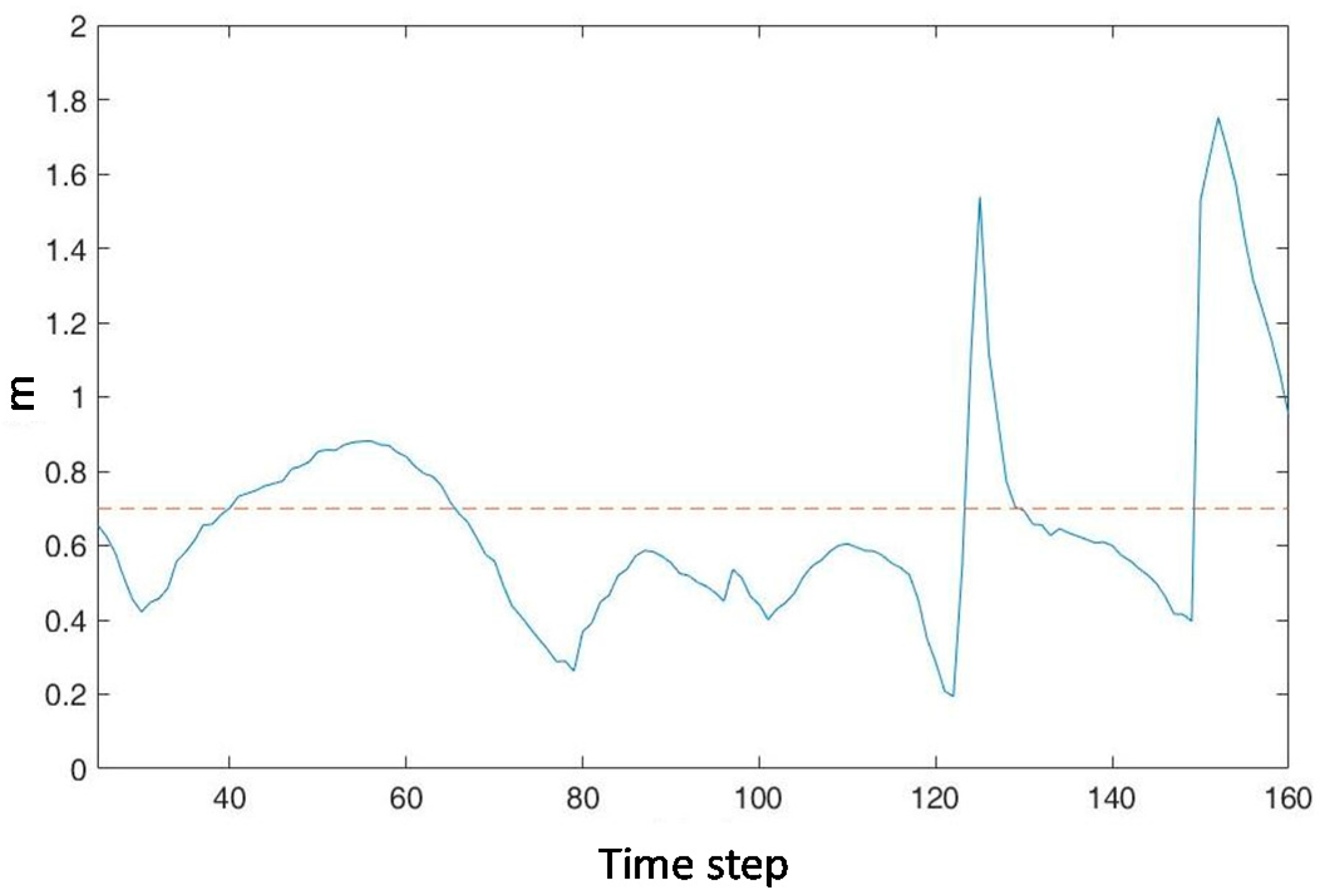
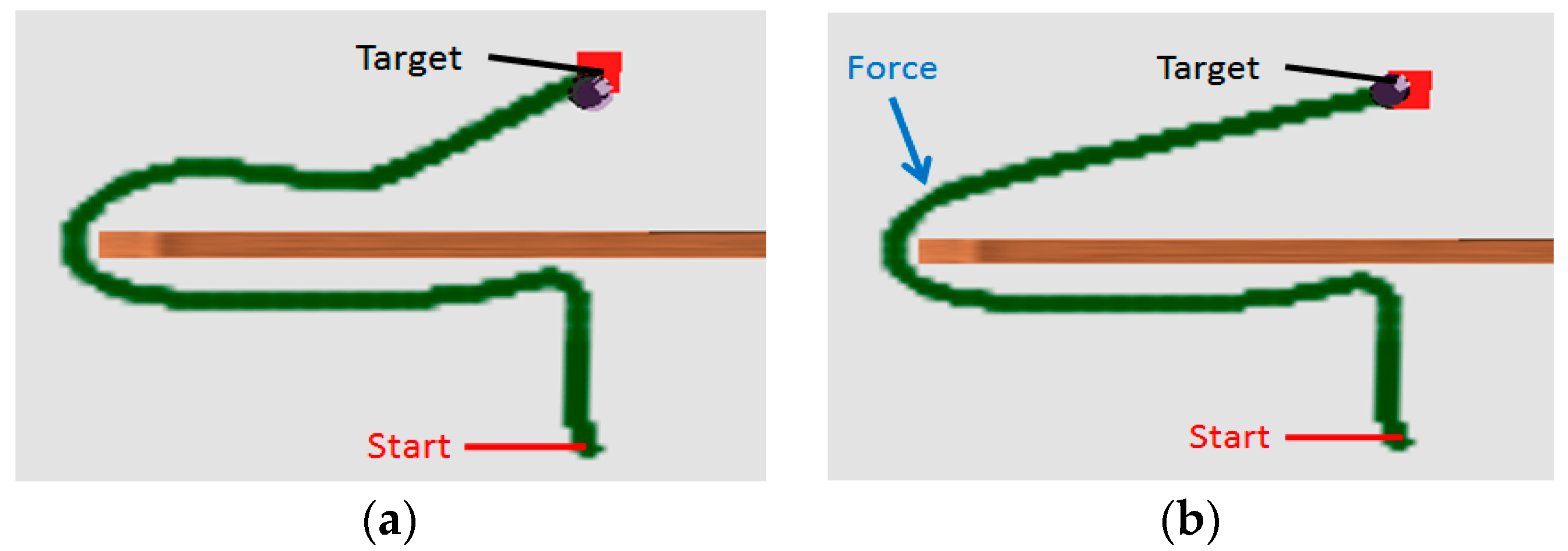
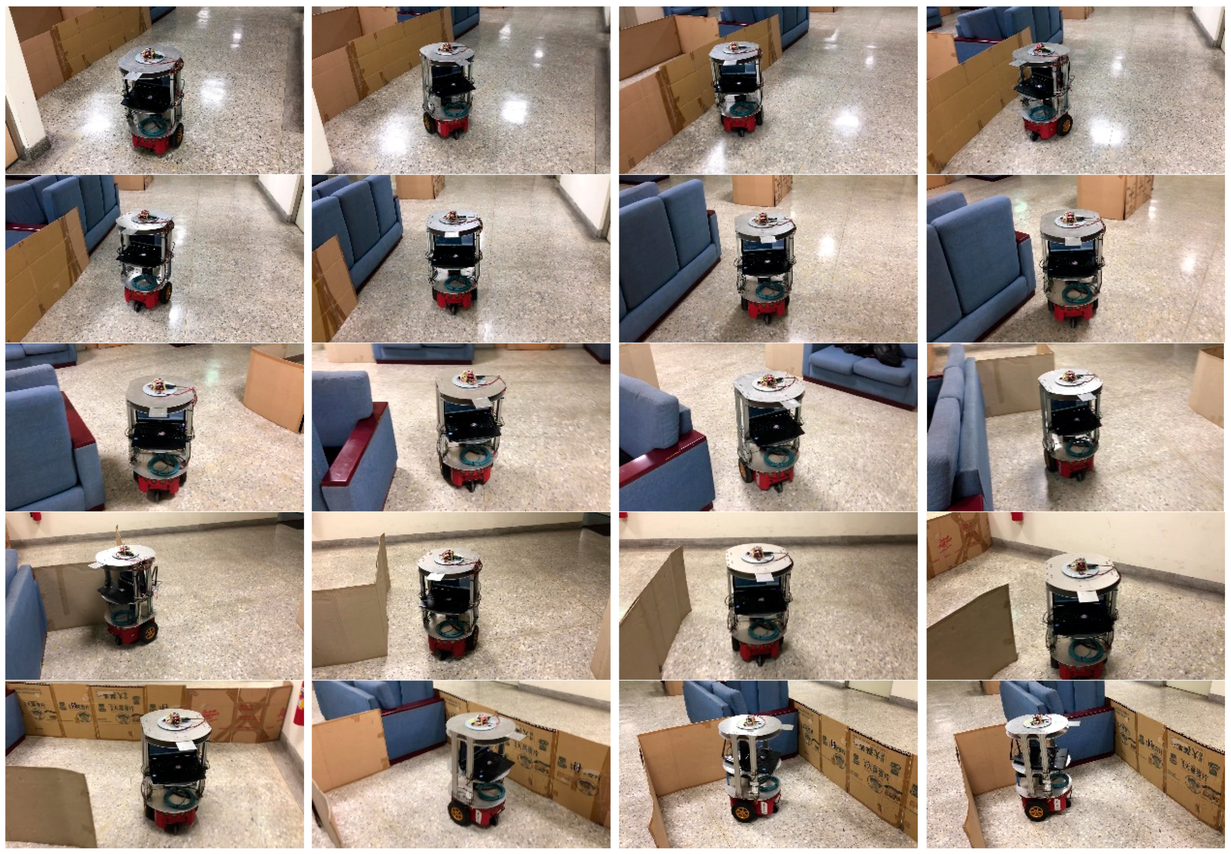
3. Results and Discussion

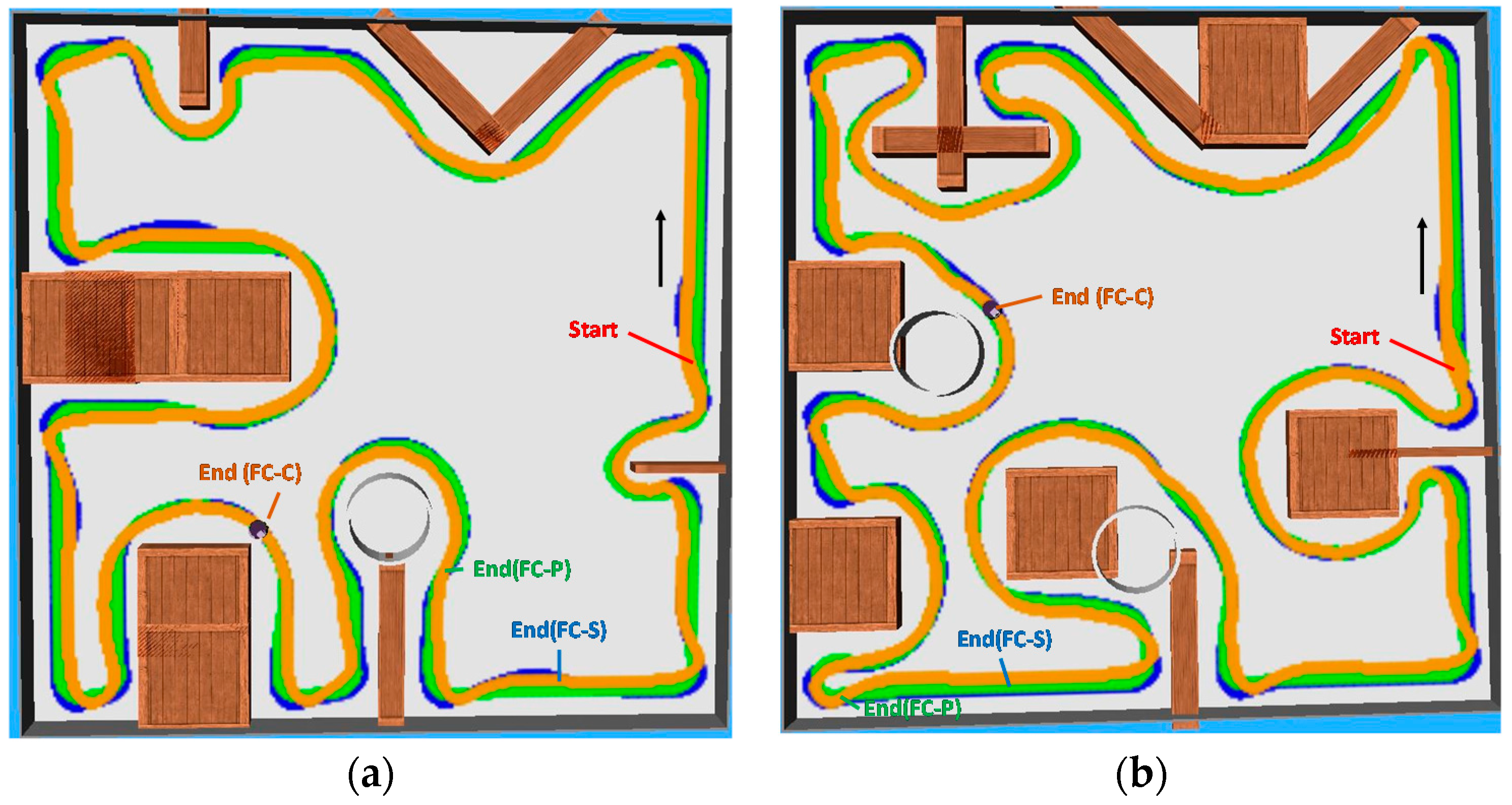
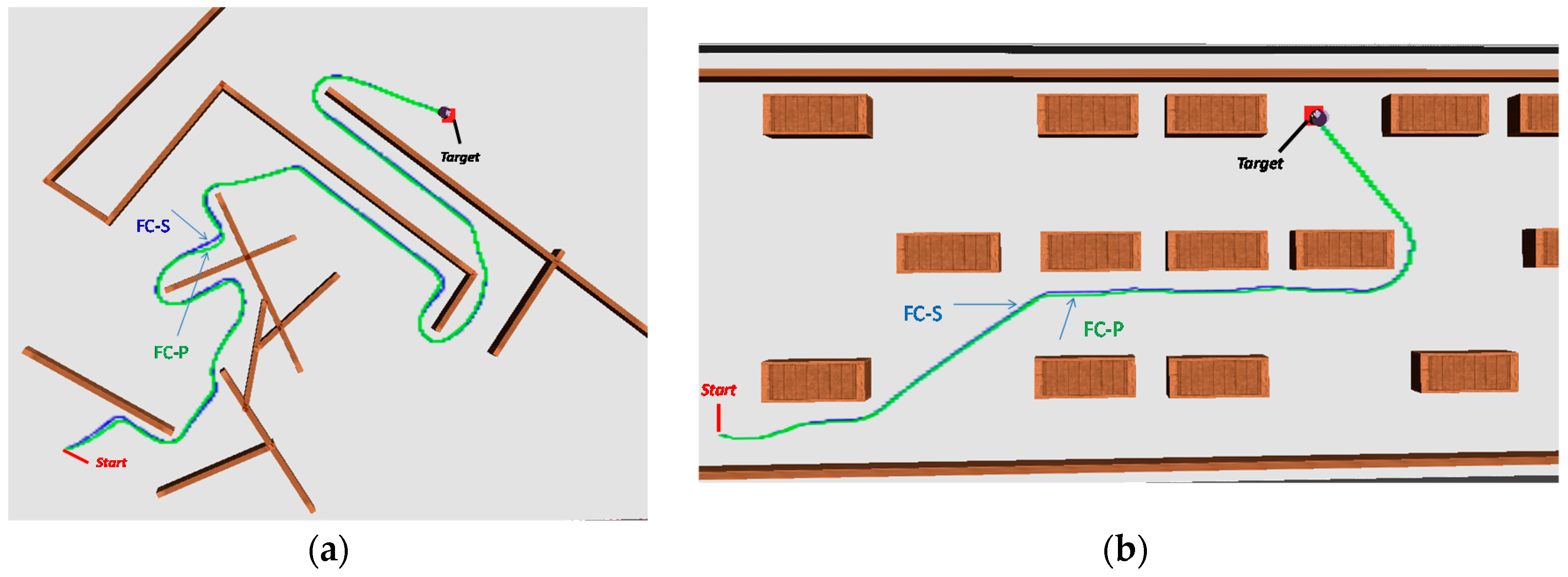
3.1. Simulations

In the simulations, the FC consisted of ten rules. Therefore, a solution vector in Equation (4) contained one hundred parameters. In the MO-FCACO, the population size was N = 40. The maximum iteration number was set to 250. The simulation was performed using Webots Pro 7.4.0 (https://www.cyberbotics.com/). A Pareto set of successful FCs was obtained after the optimization process. Among the FCs, the one that achieved the minimum $f_1$ value (denoted as FC-P) and the one that achieved the minimum $f_2$ value (denoted as FC-S) were selected. Figure 9a shows the trajectories of the robot, controlled using the two selected FCs in the training environment. Figure 9b shows the trajectories of the robot, controlled using the two selected FCs in an unknown test environment. The robot successfully moved along the wall boundary using the two FCs. The results in Figure 9 show that trajectories of the FC-S controlled robot exhibited more oscillations than the FC-P controlled robot. The FC-S controlled robot moved a further distance than the FC-P controlled robot.

Figure 10a shows the navigation results from using the two FCs in two unknown environments, Figure 10a shows that the robot successfully escaped different U-shaped obstacles, moved along the boundary of thin obstacles by executing U-turns, and reached the target. Figure 10b shows another environment, similar to a parking environment, where the robot should reach a specified empty space automatically. Each square obstacle may be regarded as a parked car. The robot automatically passes through the empty parking spaces and successfully moves along neighbouring obstacles with small gaps that are too small to pass through. Finally, the robot successfully reaches the target.

For comparison, the FC design approach in [14] was applied to the same OBF task. In this design approach, the FC controlled only the orientation of the robot, with the moving speed fixed at 0.6 m/s. Figure 9 shows the trajectories of the robot controlled using the FC (denoted as FC-C) in the training and test environments. The results showed that the FC-C controlled robot moved a shorter distance than the FC-S and FC-P controlled robots. In addition, the robot could not maintain a proper robot-wall distance while turning around corners because it cannot slow down its speed. The comparison result shows the advantage of using the multi-objective FC approach in the OBF task.

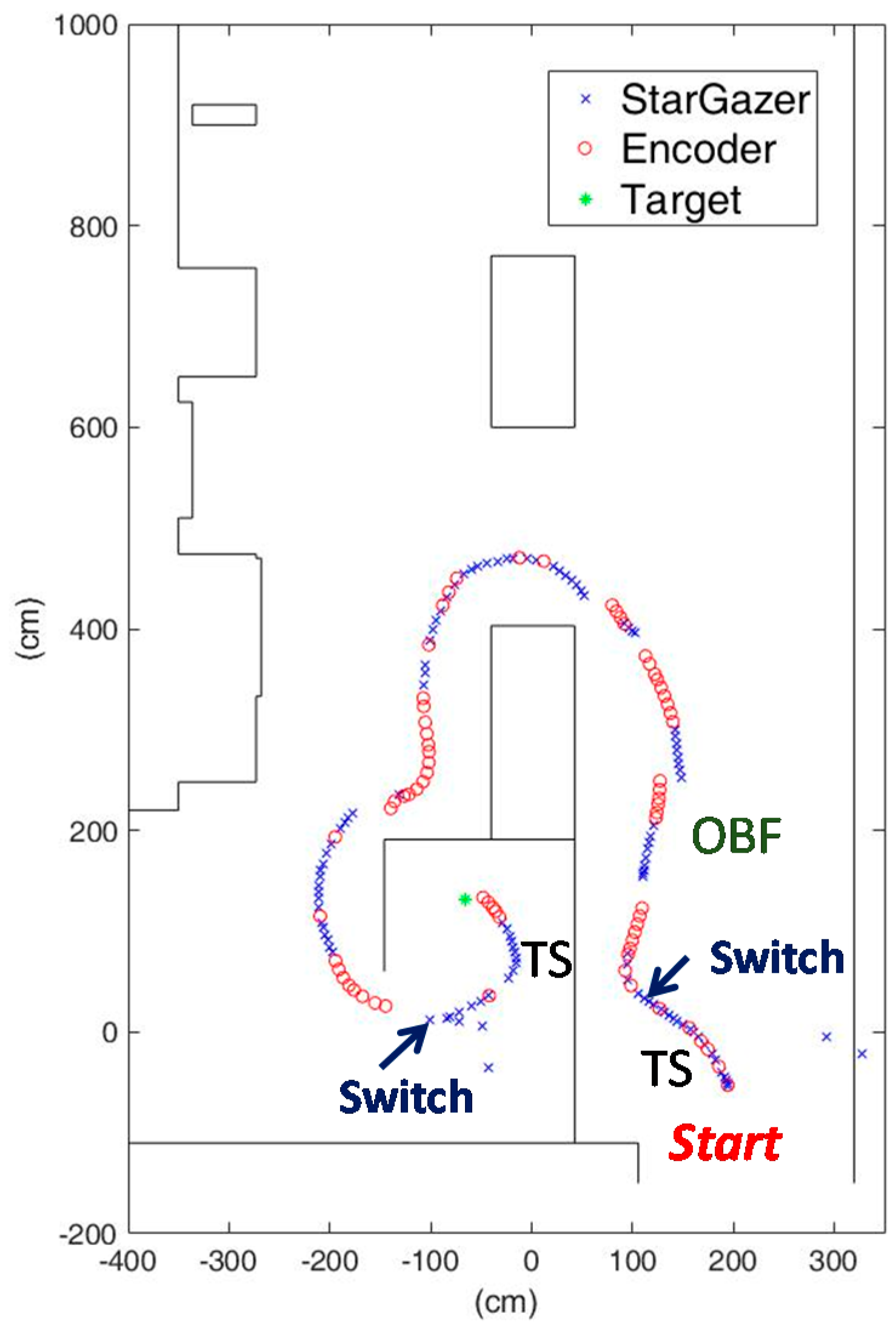
3.2. Experiments

The software-designed FC-P, together with the proposed navigation scheme, was applied to control a real Pioneer 3-DX robot. For the OBF behavior in the experiment, the four distance measurement inputs of the FC were obtained from the laser rangefinder mounted on the robot. For the TS, the robot was mainly localized using a Stargazer sensor (http://www.hagisonic.com), mounted on the top of the robot. The coordinates and orientation of the robot were determined from the measurements of the Stargazer sensor. These sensor measurements were used to find the $D_T \left(t\right)$ and ${\theta }_{TS}$ in the velocity- and orientation-PID controllers, respectively. If the StarGazer sensor failed to localize the robot at some time steps, then the encoders alone were used to estimate the robot’s location. In navigation applications, the robot must know the target to which it moves. The target can be automatically detected by the robot, such as using computer vision-based detection of the target, or manually assigned by the user. In the experiment, the coordinate of the target was manually assigned in advance. In the experiment, the robot stopped when the robot–target distance was within 10 cm. Figure 11 shows the navigation result in an unknown environment. Figure 11 shows that the Stargazer sensor signals were not available in some control intervals. In these time intervals, the robot was localized using the encoders. The robot automatically navigated to the target without a priori knowledge of the environment map. Figure 12 shows snapshots of the experimental result. Figure 13 shows the measurements of the laser sensor when the robot executed the OBF behavior in the period from time steps 25 to 160. The desired distance was $L_{wall}\left(t\right)$ = 0.7 m. The peak distance values in Figure 13 occurred when the robot moved along the outer corners with right angles. The value of the objective function $\left|L_{wall}/0.7-1\right|$ in Equation (5) over the $T_s\left(=125\right)$ steps was 0.31.

In robot and vehicle navigations, accurate positioning is important. In the above experiment, localization of the robot was implemented based on a Stargazer sensor. The localization approach is feasible in indoor environments. In the scenario of vehicle/robot navigation in outdoor environments, a different positioning method should be employed. Sensors, such as GPS, inertial measurement units, LIDAR, and cameras, have been employed for this purpose [1,2,7], as described in the introduction section.

4. Conclusions

A new navigation scheme in unknown environments was proposed in this paper. In this scheme, to avoid collision with obstacles, the robot is controlled to perform the OBF behavior. In this behavior, an FC is used and optimized through the MO-FCACO that considers the objectives of controlled position accuracy and moving speed. The MO-FCACO-based design approach avoids the time-consuming manual design of an FC and provides a Pareto set of FCs for selection. The hybrid PID controllers used in the TS behavior help to increase moving speed and reduce oscillations of the robot. The proposed navigation approach with the laser sensors considers the dead cycle problem and successfully navigates the robot to a desired target. The navigation scheme may be applied to autonomous vehicles in unknown environments.

References

- Rose, C.; Britt, J.; Allen, J.; Bevly, D. An integrated vehicle navigation system utilizing lane-detection and lateral position estimation systems in difficult environments for GPS. IEEE Trans. Intell. Transp. Syst. 2014, 15, 2615–2629. [Google Scholar] [CrossRef]
- Kim, S.B.; Bazin, J.C.; Lee, H.K.; Choi, K.H.; Park, S.Y. Ground vehicle navigation in harsh urban conditions by integrating inertial navigation system, global positioning system, odometer and vision data. IET Radar Sonar Navig. 2011, 5, 814–823. [Google Scholar] [CrossRef]
- Reyher, A.V.; Joos, A.; Winner, H. A Lidar-Based Approach for Near Range Lane Detection. In Proceedings of the 2005 IEEE Conference on Intelligent Vehicles Symposium, Las Vegas, NV, USA, 6–8 June 2005; pp. 147–152. [Google Scholar]
- Vu, A.; Ramanandan, A.; Chen, A.; Farrell, J.A.; Barth, M. Real-time computer vision/DGPS-aided inertial navigation system for lane-level vehicle navigation. IEEE Trans. Intell. Transp. Syst. 2012, 13, 899–913. [Google Scholar] [CrossRef]
- Lima, D.A.D.; Victorino, A.C. A Visual Servoing Approach for Road Lane Following with Obstacle Avoidance. In Proceedings of the 17th International IEEE Conference on Intelligent Transportation Systems (ITSC), Qingdao, China, 8–11 October 2014; pp. 412–417. [Google Scholar]
- Li, Q.; Chen, L.; Li, M.; Shaw, S.L.; Nüchter, A. A Sensor-fusion drivable-region and lane-detection system for autonomous vehicle navigation in challenging road scenarios. IEEE Trans. Veh. Technol. 2014, 63, 540–555. [Google Scholar] [CrossRef]
- Gwon, G.P.; Hur, W.S.; Kim, S.W.; Seo, S.W. Generation of a precise and efficient lane-level road map for intelligent vehicle systems. IEEE Trans. Veh. Technol. 2017, 66, 4517–4533. [Google Scholar] [CrossRef]
- Jiang, Y.; Zhao, H.; Fu, H. A Control Method to Avoid Obstacles for an Intelligent Car Based on Rough Sets and Neighborhood Systems. In Proceedings of the 10th International Conference on Intelligent Systems and Knowledge Engineering (ISKE), Taipei, Taiwan, 24–27 November 2015; pp. 66–70. [Google Scholar]
- Cupertino, F.; Giordano, V.; Naso, D.; Delfine, L. Fuzzy control of a mobile robot. IEEE Robot. Autom. Mag. 2006, 13, 74–81. [Google Scholar] [CrossRef]
- Farooq, U.; Hasan, K.M.; Raza, A.; Amar, M.; Khan, S.; Javaid, S. A Low Cost Microcontroller Implementation of Fuzzy Logic Based Hurdle Avoidance Controller for a Mobile Robot. In Proceedings of the 2010 3rd IEEE International Conference on Computer Sciences and Information Technology, Chengdu, China, 9–11 July 2010; pp. 480–485. [Google Scholar]
- Farooq, U.; Hasan, K.M.; Amar, M.; Asad, M.U. Design and Implementation of Fuzzy Logic Based Autonomous Car for Navigation in Unknown Environments. In Proceedings of the 2013 International Conference on Informatics, Electronics and Vision (ICIEV), Dhaka, Bangladesh, 17–18 May 2013; pp. 1–7. [Google Scholar]
- Tao, T. Fuzzy Automatic Driving System for a Robot Car. In Proceedings of the 2014 International Conference on Fuzzy Theory and Its Applications (iFUZZY2014), Kaohsiung, Taiwan, 26–28 November 2014; pp. 132–137. [Google Scholar]
- Juang, C.F.; Hsu, C.H. Reinforcement ant optimized fuzzy controller for mobile-robot wall-following control. IEEE Trans. Ind. Electron. 2009, 56, 3931–3940. [Google Scholar] [CrossRef]
- Juang, C.F.; Chang, Y.C. Evolutionary group-based particle swarm-optimized fuzzy controller with application to mobile robot navigation in unknown environments. IEEE Trans. Fuzzy Syst. 2011, 19, 379–392. [Google Scholar] [CrossRef]
- Juang, C.F.; Jeng, T.L.; Chang, Y.C. An interpretable fuzzy system learned through online rule generation and multi-objective ACO with a mobile robot control application. IEEE Trans. Cybern. 2016, 46, 2706–2718. [Google Scholar] [CrossRef] [PubMed]
- Korf, R.E. Depth-first iterative-deepening: An optimal admissible tree search. Artif. Intell. 1985, 27, 97–109. [Google Scholar] [CrossRef]
- Koenig, S.; Likhachev, M.; Furcy, D. Lifelong planning A*. Artif. Intell. 2004, 155, 93–146. [Google Scholar] [CrossRef]
- Daniel, K.; Nash, A.; Koenig, S.; Felner, A. Theta*: Any-angle path planning on grids. J. Artif. Intell. Res. 2010, 39, 533–579. [Google Scholar]
- Zhong, C.; Liu, S.; Lu, Q.; Zhang, B.; Yang, S.X. An efficient fine-to-coarse wayfinding strategy for robot navigation in regionalized environments. IEEE Trans. Cybern. 2016, 46, 3157–3170. [Google Scholar] [CrossRef] [PubMed]
- Zalama, E.; Gomez, J.; Paul, M.; Peran, J.R. Adaptive behavior navigation of a mobile robot. IEEE Trans. Syst. Man Cybern. Part A Syst. Hum. 2002, 32, 160–169. [Google Scholar] [CrossRef]
- Rusu, P.; Petriu, E.M.; Whalen, T.E.; Cornell, A.; Spoelder, H.J.W. Behavior-based neuron-fuzzy controller for mobile robot navigation. IEEE Trans. Instrum. Meas. 2003, 52, 1335–1340. [Google Scholar] [CrossRef]
- Hui, N.B.; Mahendar, V.; Pratihar, D.K. Time-optimal, collision free navigation of a car-like mobile robot using neuro-fuzzy approaches. Fuzzy Sets Syst. 2006, 157, 2172–2204. [Google Scholar] [CrossRef]
- Zhu, A.; Yang, S.X. Neurofuzzy-based approach to mobile robot navigation in unknown environments. IEEE Trans. Syst. Man Cybern. Part C (Appl. Rev.) 2007, 37, 610–621. [Google Scholar] [CrossRef]
- Jolly, K.G.; Sreerama Kumar, R.; Vijayakumar, R. Intelligent task planning and action selection of a mobile robot in a multi-agent system through a fuzzy neural network approach. Eng. Appl. Artif. Intell. 2010, 23, 923–933. [Google Scholar] [CrossRef]
- Antonelo, E.A.; Schrauwen, B. On Learning Navigation Behaviors for Small Mobile Robots With Reservoir Computing Architectures. IEEE Trans. Neural Netw. Learn. Syst. 2015, 26, 763–780. [Google Scholar] [CrossRef] [PubMed]
- Brahimi, S.; Tiar, R.; Azouaoui, O.; Lakrouf, M.; Loudini, M. Car-Like Mobile Robot Navigation in Unknown Urban Areas. In Proceedings of the 2016 IEEE 19th International Conference on Intelligent Transportation Systems (ITSC), Rio de Janeiro, Brazil, 1–4 November 2016; pp. 1727–1732. [Google Scholar]
- Yoon, S.W.; Park, S.B.; Kim, J.S. Kalman filter sensor fusion for mecanum wheeled automated guided vehicle localization. J. Sens. 2015, 2015, 347379. [Google Scholar] [CrossRef]
- Deb, K.; Pratap, A.; Agarwal, S.; Meyarivan, T. A fast and elitist multiobjective genetic algorithm: NSGAII. IEEE Trans. Evol. Comput. 2002, 6, 182–197. [Google Scholar] [CrossRef]
© 2018 by the authors. Licensee MDPI, Basel, Switzerland. This article is an open access article distributed under the terms and conditions of the Creative Commons Attribution (CC BY) license (http://creativecommons.org/licenses/by/4.0/).
Share and Cite
Chou, C.-Y.; Juang, C.-F. Navigation of an Autonomous Wheeled Robot in Unknown Environments Based on Evolutionary Fuzzy Control. Inventions 2018, 3, 3. https://doi.org/10.3390/inventions3010003
Chou C-Y, Juang C-F. Navigation of an Autonomous Wheeled Robot in Unknown Environments Based on Evolutionary Fuzzy Control. Inventions. 2018; 3(1):3. https://doi.org/10.3390/inventions3010003
Chicago/Turabian StyleChou, Ching-Yu, and Chia-Feng Juang. 2018. "Navigation of an Autonomous Wheeled Robot in Unknown Environments Based on Evolutionary Fuzzy Control" Inventions 3, no. 1: 3. https://doi.org/10.3390/inventions3010003
APA StyleChou, C.-Y., & Juang, C.-F. (2018). Navigation of an Autonomous Wheeled Robot in Unknown Environments Based on Evolutionary Fuzzy Control. Inventions, 3(1), 3. https://doi.org/10.3390/inventions3010003