1. Introduction
Programmable Logic Controllers (PLCs) are the standard intelligence for instrumentation and control systems utilised in process control and are used in a wide variety of industries from car manufacturing to building management systems, as well as controlling machinery in large mine sites [
1]. PLCs often form the basis of many automated industrial processes and are essentially the heart of a Supervisory Control And Data Acquisition (SCADA) system. A PLC is an electro-mechanical computer specifically designed to take in information from a multitude of sensors in real-world industrial processes and react to those sensing inputs by controlling actuators in such a way as defined by the control logic [
2]. For example, a PLC may receive data corresponding to the pressure of a fluid in a pipeline and then react to that signal by sending a command to the field to open a valve, stop a pump, sound an alarm, or any other action, depending on what is required. Currently, there is a number of different communication protocols and sensing standards for automated processes, such as Profibus [
3] and Foundation Fieldbus [
4], as well as an array of smaller proprietary protocols. The particular standards used in any one process depend on a number of factors, from the size of the plant to the scale of automation required and the PLC manufacturer. One of the traditional analogue input sensing standards is 4–20 mA [
5]. The physical signal from an analogue sensor to the PLC is between 4 mA and 20 mA, where 4 mA corresponds to 0% and 20 mA corresponds to 100% of the measurand. The main advantage of using this technique is that a faulty connection can be detected easily, as it will result in the PLC receiving 0 mA.
As with PLCs, optical fibre sensors are now used in a large variety of diverse applications and are capable of measuring many different types of signals, both static and dynamic, including temperature, pressure, level and flow, as well as chemical and biological measurands [
6,
7,
8]. It is well recognized that optical fibre sensors have many desirable attributes, which are advantageous with respect to other sensing methodologies, which include greater sensitivity, reduced size and weight and immunity to electromagnetic interference. However, in general, optical fibre sensors are underutilised in process control applications. There are a number of reasons for this lack of penetration into mainstream industrial processes. These include the cost and complexity of optical fibre-based sensing systems, as well as the fact that simpler traditional sensing techniques based on well-established industrial standards are, to date, usually preferred. The use of optical fibre systems is increasing in some industrial applications, for both information transmission and sensing, since these systems are immune to electromagnetic interference and offer faster data transmission rates [
9]. It has been proposed that signals from optical fibre sensors used in real-time industrial applications could be monitored with PLCs [
10]. However, whilst most major PLC manufacturers now offer an optical fibre interface for communications, they do not enable optical fibre sensors to be connected directly to PLC I/O cards.
Where fibre optic sensors are used in process control applications, the sensors are usually on the end of an optical fibre, where the fibre is simply used as the data transmission medium. This method completely underutilizes many of the advantages of the fibre itself. A signal conditioning system was demonstrated however for optically identical Fabry-Perot sensors, capable of detecting different measurands in industrial applications [
11]. Fibre Bragg Grating (FBG) sensors are also optical fibre-based sensors that have the advantage of being able to be multiplexed and hence can form a distributed sensing network, rather than a single sensor on the end of a line. Some of the multiplexing architectures are described in [
12]. FBG sensors were first reported by Morey, Meltz and Glenn in 1989 [
13], but they became widely accessible, after they demonstrated their transverse holographic fabrication method for FBGs [
14]. Initially, FBGs were used as spectral transduction elements, whereby the sensing information corresponded directly to the wavelength shift of the FBG. As such, they can be implemented in Wavelength Division Multiplexing (WDM) or Time Division Multiplexing (TDM) systems [
15]. Unfortunately, these systems require spectral decoding of the sensor signals, which can be costly and processor intensive.
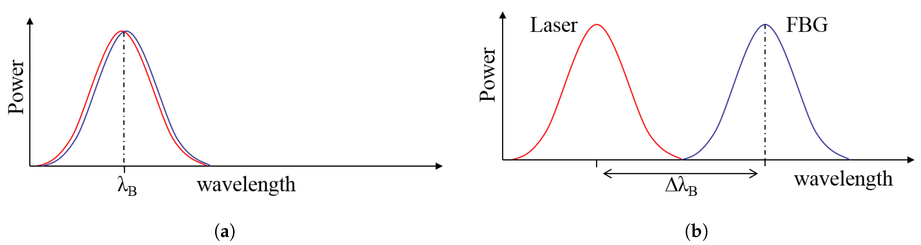
A more efficient alternative is to use FBGs in an intensity-based detection system where the relative spectral shift in the FBG filter results in an optical power change, which in turn correlates with a change in the measurand [
16]. This relatively simple interrogation technique can be used to convert the change in the measurand from the optical domain to the electrical domain, meaning they can easily be integrated into existing control system architectures without the need for expensive stand-alone optical interrogators. The disadvantage of intensity-based detection systems is that input optical power fluctuations are introduced. However, the simplicity of the interrogation of the signal and the reduced cost greatly outweigh the corresponding disadvantages in certain low frequency applications, such as in the process control industry.
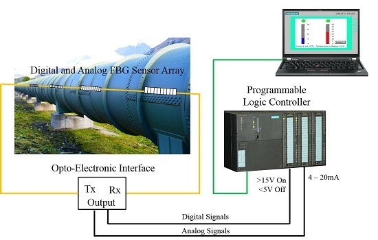
Here, we show that the output from both digital and analogue optical fibre sensors can be interfaced with a PLC I/O rack. The output from an FBG-based optical switch can be interfaced with a digital input card on a PLC, and the output from a FBG temperature sensor can be interfaced to a standard 4–20 mA analogue input card on a PLC. This technique enables optical fibre sensors to be directly compatible with current industry standards for PLC systems.
3. PLC Fibre Optic Sensor Digital Input Interface
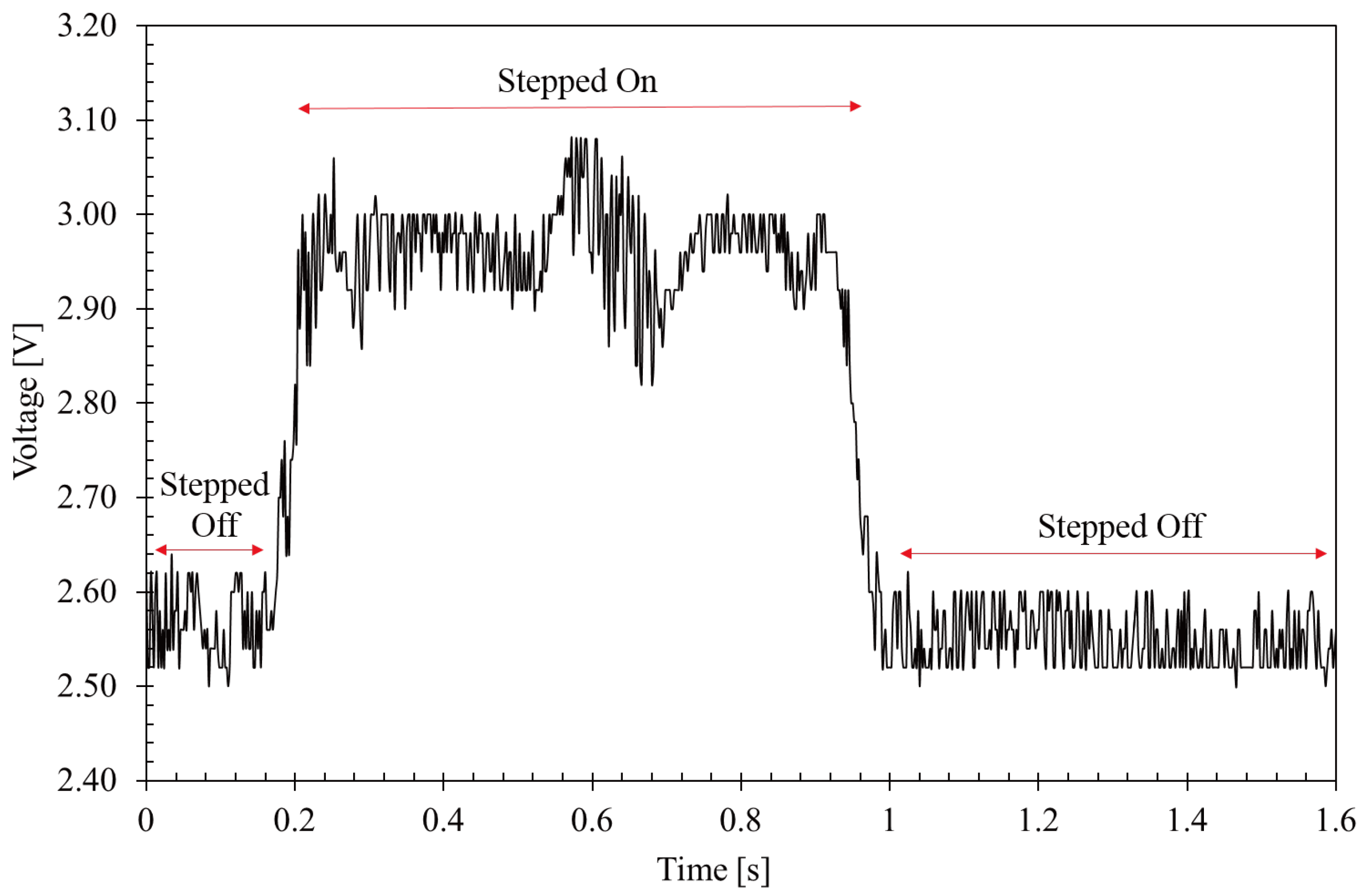
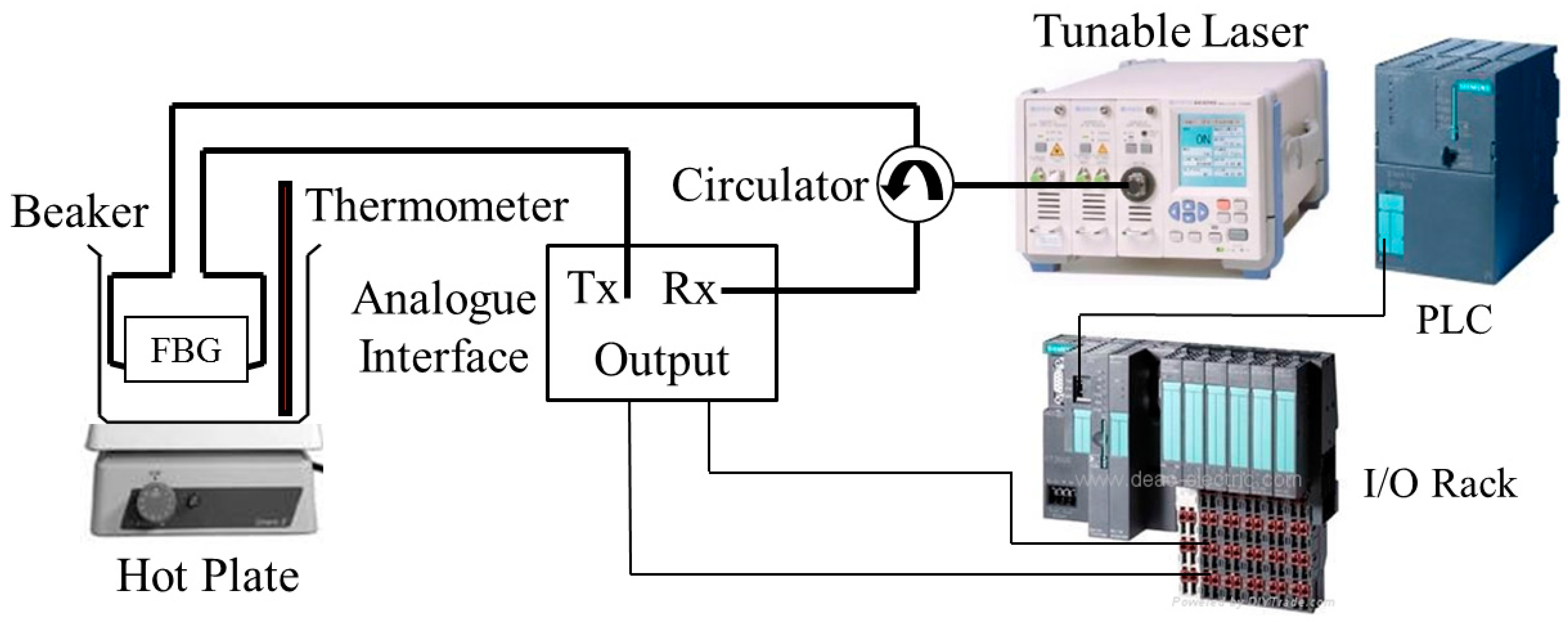
Here, a PLC Fibre Optic Sensor (FOS) digital input interface is demonstrated. An in-ground FBG pressure switch, previously reported in [
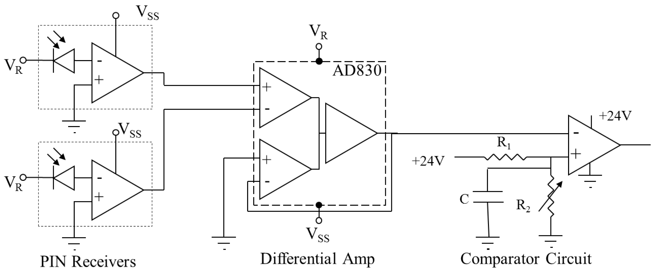
24], whereby a 60-kg person stepped on a floorboard with the FBG bonded beneath it creating a voltage swing of approximately 0.5 V, was used as an arbitrary digital input signal for a PLC (Siemens S7-300, Munich, Germany). The Bragg wavelength of the FBG and the central wavelength of the laser were initially matched. As pressure was applied to the FBG, the Bragg wavelength shifted away from the laser’s position, producing an increase in transmitted optical power and a decrease in the reflected power, before returning back to its original position when it was stepped off.The PLC can be programmed to ensure the switch is latched on, so that the output alarm from the PLC would stay on until it is reset. As a PLC’s scan time is of the order of milliseconds, it would capture an increase in signal even if it then decreased.A bench-top tunable laser (Anritsu MG9637A, Kanagawa, Japan) was connected to the FBG (Micron Optics OS1100, Atlanta, GA, USA) via an optical circulator (FDK YC-1100-155, Tokyo, Japan). The reflected signal was directed down to the first photoreceiver (Fujitsu FRM3Z231KT, Tokyo, Japan) via the optical circulator, and the signal was transmitted through the FBG and was directed to the second receiver (Fujitsu FRM3Z231KT, Tokyo, Japan). The output of the two receivers was differentially amplified using a high speed differential amplifier (AD830ANZ, Norwood, MA, USA). The result is shown in
Figure 3.
A simple comparator circuit was then used to ensure the differentially-amplified output voltage would be correctly interpreted by the PLC. The output from the comparator was then connected to a two-channel, 24-V digital input module on the I/O rack (Siemens ET200S, Munich, Germany). The digital input card detects a one when the input voltage is above 15 V, and it detects a zero when the input voltage is below 5 V. Hence, the 0.5-V swing, which occurred when the switch was stepped on was converted to a change of more than 10 V to ensure the value read by the PLC changed from a zero to a one. The transimpedance amplifier supply and the PIN bias for the two receivers was provided by a ±5-V DC power supply. The 24 V for the comparator circuit would be supplied by the PLC. The PLC FOS digital input interface circuit diagram is shown in
Figure 4.
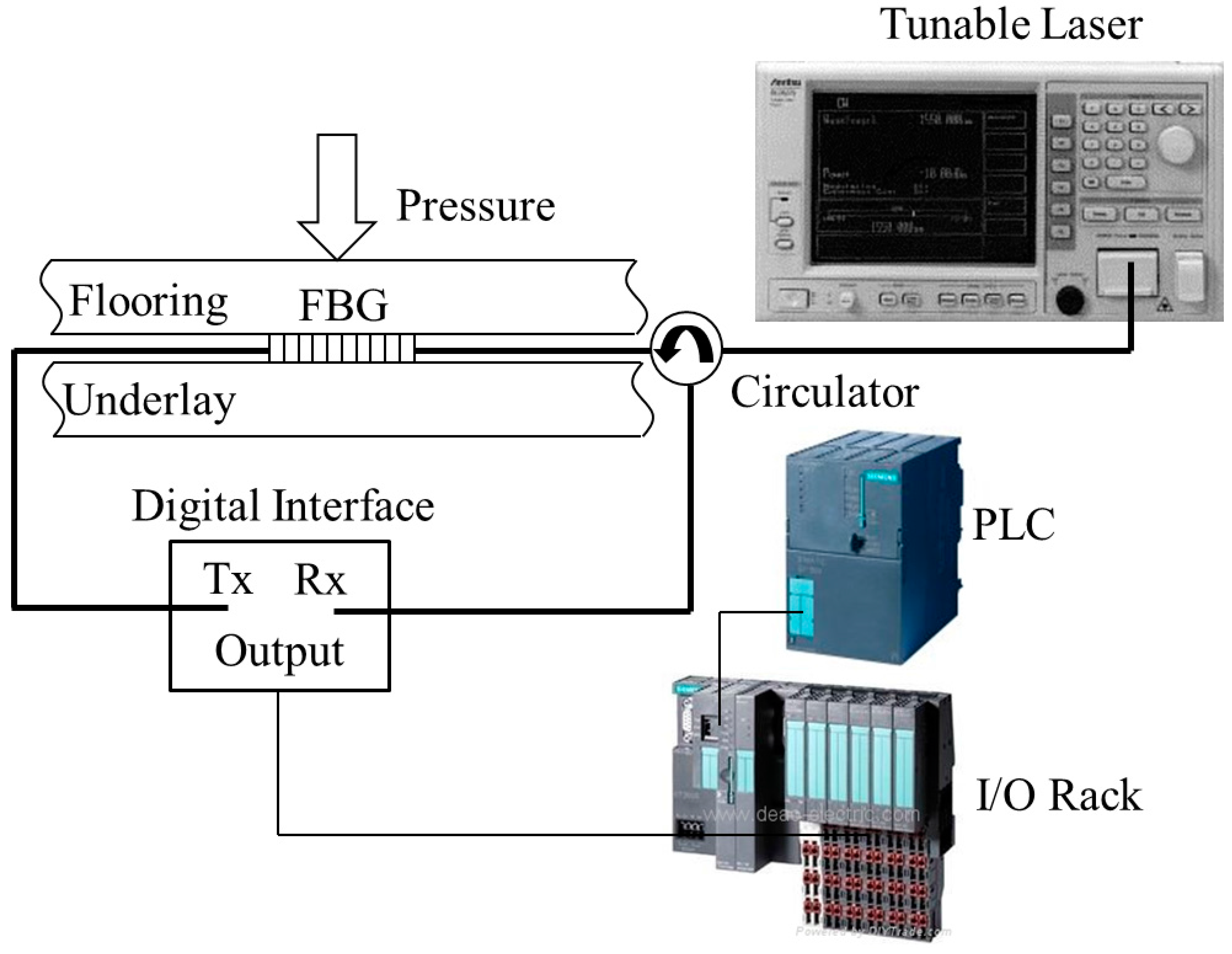
The in-ground pressure switch provided the digital signal for the PLC FOS digital input interface, which was connected to the digital input channel on the Siemens S7-300 PLC I/O rack. The experimental setup is shown in
Figure 5.
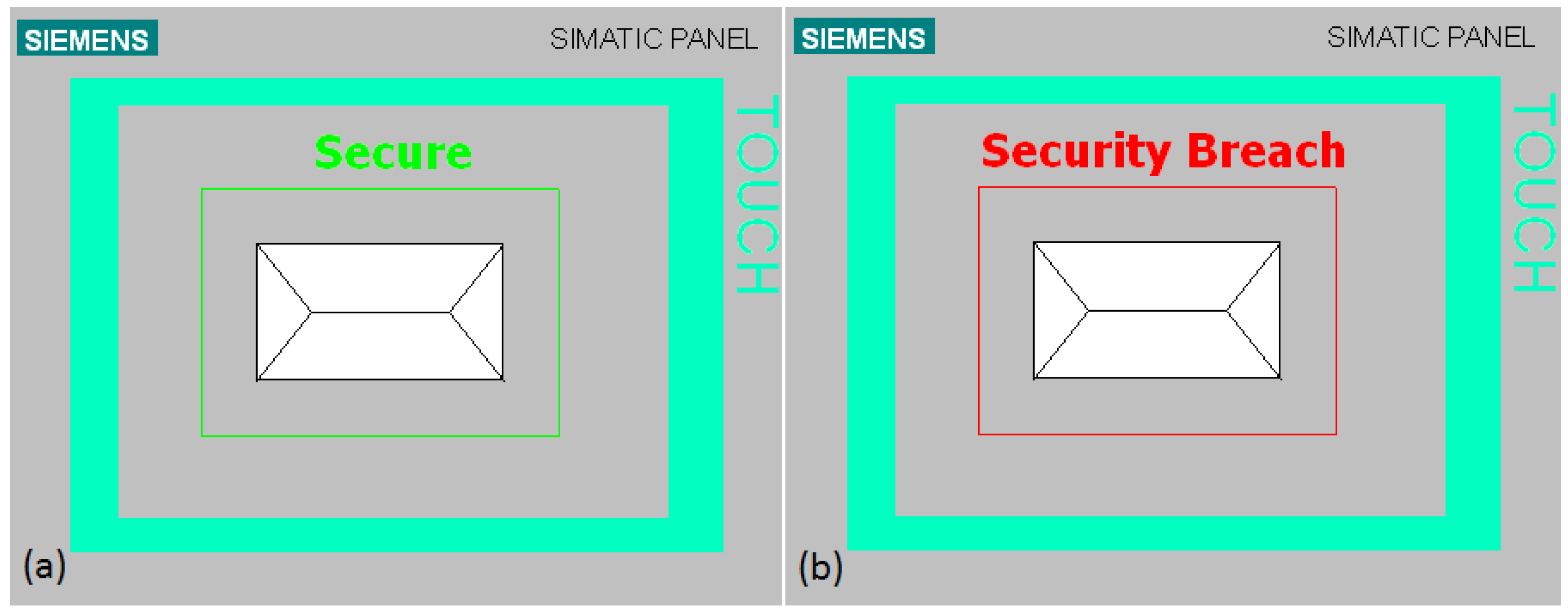
A simple Physical Intrusion Detection System (PIDS)-based Human Machine Interface (HMI), created using WinCC Flexible software [
25], was designed to display the alarm event.
Figure 6 shows the HMI display when the perimeter is secure and when a security breach has occurred.
4. PLC FOS Analogue Input Interface
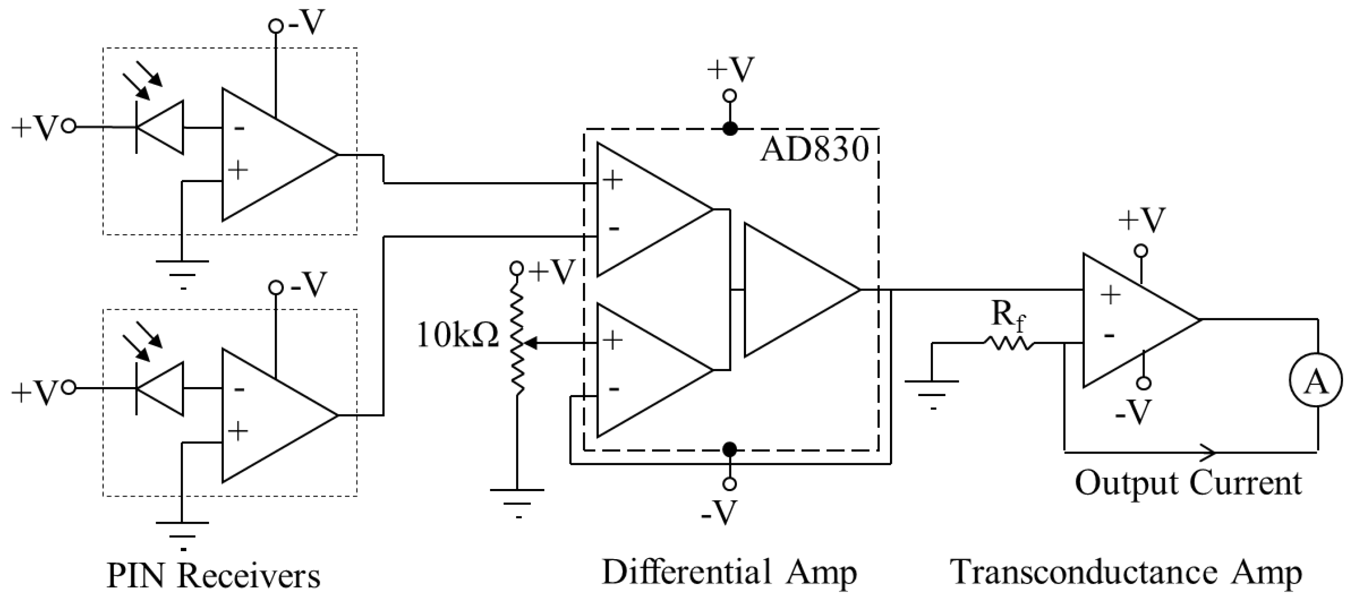
Here, a PLC FOS analogue input interface is demonstrated. The experimental setup was similar to the previous setup, except a bench-top tunable laser module (Ando AQ 8201-13B, Tokyo, Japan) was used instead of the Anritsu MG9637A tunable laser. Again, the output of the two receivers was differentially amplified using a high speed differential amplifier (AD830ANZ, Norwood, MA, USA). An additional 3-V DC offset was supplied to the second summing input of the difference amplifier via a voltage divider from the +5 V. The DC offset was used due to the requirements of the transconductance amplifier. The transconductance amplifier converts a voltage range of 1 V–5 V into 4 mA–20 mA, as required by the PLC. This requires a bias resistance of 250
, giving 4 mA at 1 V and 20 mA at 5 V and, therefore, a midpoint of 3 V. The transimpedance amplifier (current-to-voltage converter) supply, PIN bias for the two receivers and the supply for the transconductance amplifier (voltage-to-current converter) was provided by a ±5 V DC power supply.
Figure 7 shows the circuit diagram of the PLC FOS analogue input interface.
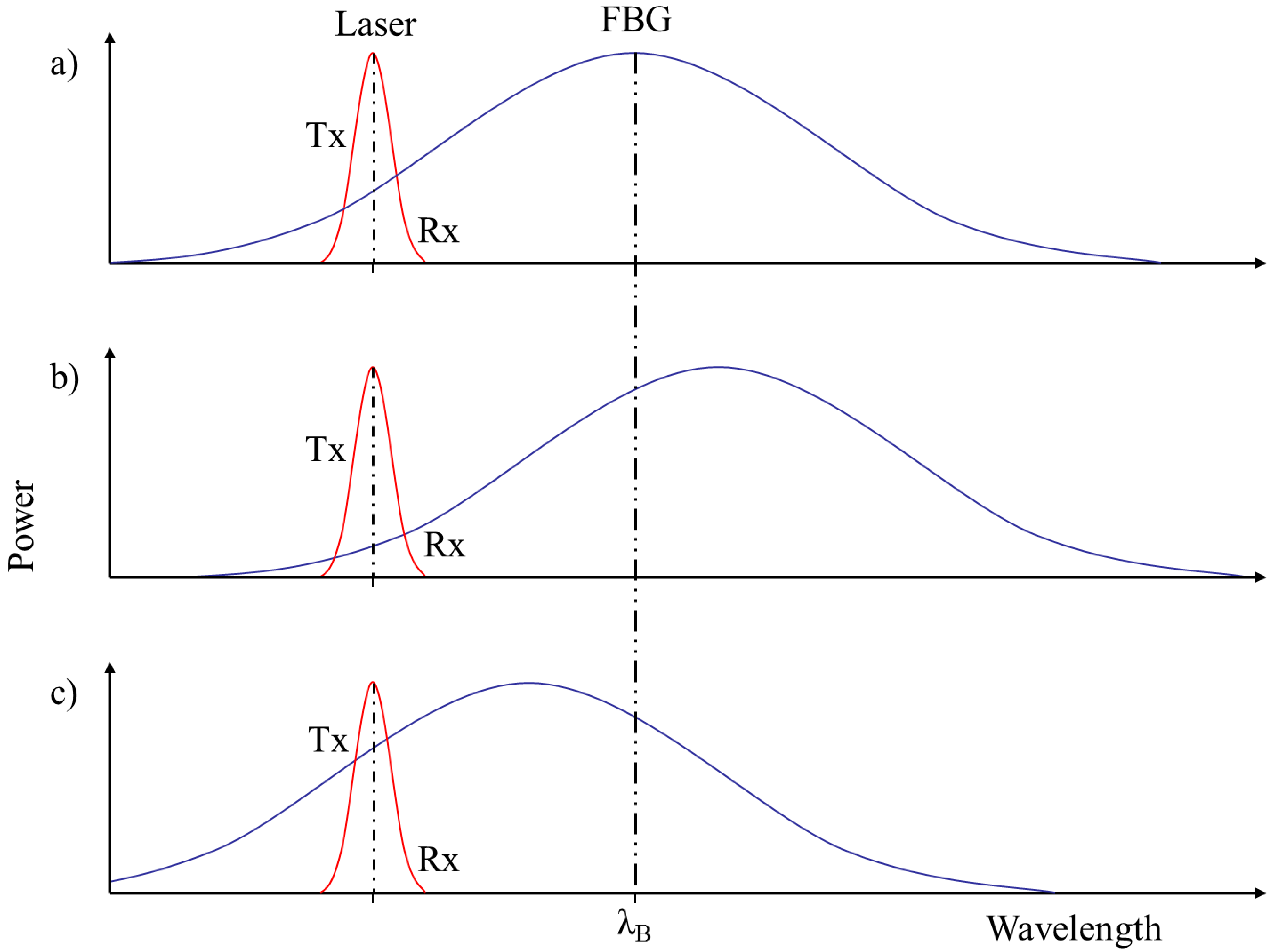
Initially, the spectral characteristics of the FBG needed to be measured, and the tunable laser needed to be set to the correct wavelength, in order to determine the operating point for the FBG sensor. The laser was initially tuned to the minimum reflectivity above the Bragg wavelength to ensure that all the optical power was transmitted through the FBG.
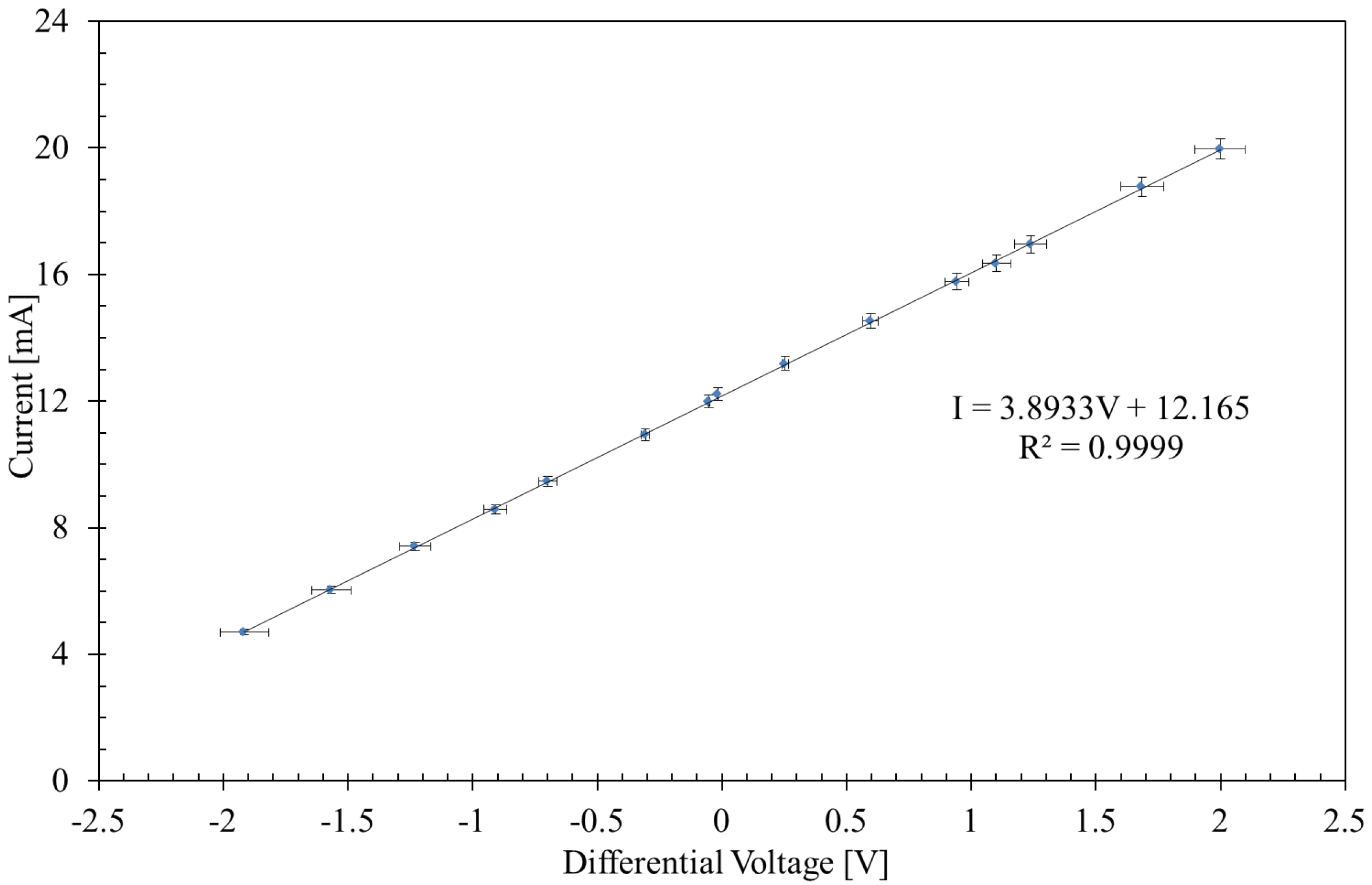
Prior to utilizing the optical input with the two transimpedance amplifiers, two function generators (Agilent 33250A, Santa Clara, CA, USA) were used, each set to give a negative voltage, similar to those expected from the transimpedance amplifiers. Initial tests showed the voltage of each receiver varied from −1 V–−2 V, for zero to maximum optical power (8 mW) of the tunable laser. The output of the difference amplifier was then between −1 V and 1 V, and with the 3-V offset, it then gave an expected 2 V–4 V output voltage to the transconductance amplifier, which corresponded to an expected output current of 8 mA–16 mA. To test the entire range of the system, the function generator output voltages were varied between −2.5 V and 0.5 V, to give an output current of 4 mA–20 mA, measured using a Digital Multimeter (DMM) (Goldstar DM-331, Seoul, Korea).
Figure 8 shows the transfer function of the transconductance amplifier. As shown, the transfer function is extremely linear, where the gradient is
mA/V and the intercept is
mA. There is a small discrepancy in the equation coefficient and offset, as we would expect the values for the gradient and intercept to be exactly 4 mA/V and 12 mA, respectively. The reason for this small inconsistency is most likely due to uncertainties in the voltage offset value,
V, and the feedback resistance,
, used in the transconductance amplifier circuit. Moreover, there is a small uncertainty in the precision of the DMM,
mA and
V, when measuring the current and voltage, respectively.
For the test experiment to monitor temperature, the FBG and a thermometer (Brannan 44/430/0, Cleator Moor, UK) were placed in a large beaker of water. The FBG was then connected to the optical circuit as before, and the water was then slowly heated using a hotplate (Industrial Equipment and Control PTY CH2093). The transmitted and reflected signals were connected to the optoelectronic PLC interface, and the output current was monitored on a DMM (Escort EDM168A, Santa Rosa, CA, USA) as a function of the temperature, before being connected to an analogue input channel on the Siemens S7-300 PLC I/O rack. The setup for the temperature measurement is show in
Figure 9.
Figure 10 shows the output current from the complete circuit (
Figure 7) as a function of the applied temperature to the FBG sensor. The curve is a sigmoid, or half a Gaussian, as we would expect. This is because both the laser and FBG are Gaussian in shape, and when multiplied together, the result is a Gaussian. The amplitude of this Gaussian increases from minimum to maximum. The optical power of the laser was such that the value of the voltage varied from minus 1.2 V to positive 0.2 V, corresponding to a change in current of approximately 6 mA, from 6.97 mA–12.81 mA. The asymmetry was due to the use of a temporary bare-fibre-connector, instead of a standard pigtail connector, adding more loss in the reflected path compared to the transmitted path. With the use of connectorised components, this would no longer be an issue. The straight line between 8.02 mA and 12.01 mA, where the gradient is
mA/V and the intercept is
mA, shows the region where the output current is linear with respect to temperature. Hence, in practice, this particular setup could be used as a temperature sensor with a range from approximately 22–30
C with higher precision than the thermometer used here, which had an uncertainty of ±0.5
C. A change of 0.1 mA detected by the PLC would be a result of a change in temperature of approximately 0.2
C.
The PLC was again programmed in ladder logic and a graphical representation of the input current to the PLC and the output temperature was created using WinCC Flexible software [
25]. The direct readout from the analogue input module was converted into 4–20 mA, which was then converted into the actual temperature range, in the PLC logic. To achieve the conversion from current to temperature, the data from
Figure 10 in the linear region were plotted with temperature as a function of current. The transfer function,
, then became,
where
I is the current in mA and
T is the temperature in
C. However, because the PLC can be programmed to perform complex operations, all of the data could be converted from current to temperature. Hence, the transfer function was estimated from a multiple regression fit, by selecting a third order polynomial
,
This was then used in the PLC software (Sematic Step7, Munich, Germany) to compute the temperature across a larger dynamic range. Although this may not be possible across the full range from 14–36
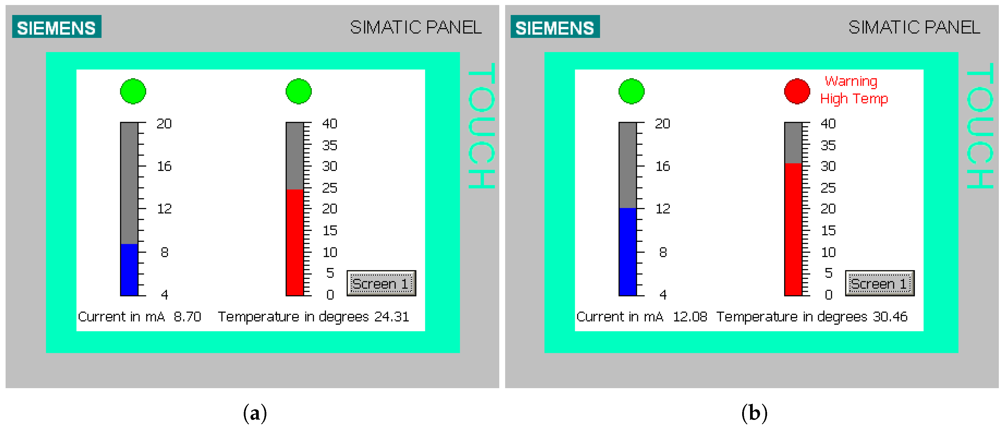
C due to the error bars, the dynamic range can be increased in this way as the PLC is capable of referring to a lookup table and interpolating results, so a linear response is not necessary. Both the current and the temperature were displayed in real time on bar graphs on the HMI, shown in
Figure 11.
Figure 11a shows an image of the HMI with the temperature in the normal operating range. Additionally, an alarm was programmed to be displayed when the temperature exceeded 30 degrees Celsius. This event is shown in
Figure 11b.


