Singular Mean-Field States: A Brief Review of Recent Results


1
Department of Physical Electronics, School of Electrical Engineering, Faculty of Engineering, Tel Aviv University, Tel Aviv 69978, Israel
2
Center for Light-Matter Interaction, Tel Aviv University, Tel Aviv 69978, Israel
3
Department of Applied Science for Electronics and Materials, Interdisciplinary Graduate School of Engineering Sciences, Kyushu University, Kasuga, Fukuoka 816-8580, Japan
*
Author to whom correspondence should be addressed.
Condens. Matter 2020, 5(1), 20; https://doi.org/10.3390/condmat5010020
Submission received: 23 February 2020
/
Revised: 15 March 2020
/
Accepted: 16 March 2020
/
Published: 20 March 2020
(This article belongs to the Special Issue Fluctuations and Highly Non-linear Phenomena in Superfluids and Superconductors II)
Abstract
:This article provides a focused review of recent findings which demonstrate, in some cases quite counter-intuitively, the existence of bound states with a singularity of the density pattern at the center; the states are physically meaningful because their total norm converges. One model of this type is based on the 2D Gross–Pitaevskii equation (GPE), which combines the attractive potential and the quartic self-repulsive nonlinearity, induced by the Lee–Huang–Yang effect (quantum fluctuations around the mean-field state). The GPE demonstrates suppression of the 2D quantum collapse, driven by the attractive potential, and emergence of a stable ground state (GS), whose density features an integrable singularity at . Modes with embedded angular momentum exist too, but they are unstable. A counter-intuitive peculiarity of the model is that the GS exists even if the sign of the potential is reversed from attraction to repulsion, provided that its strength is small enough. This peculiarity finds a relevant explanation. The other model outlined in the review includes 1D, 2D, and 3D GPEs, with the septimal (seventh-order), quintic, and cubic self-repulsive terms, respectively. These equations give rise to stable singular solitons, which represent the GS for each dimension D, with the density singularity . Such states may be considered the results of screening a “bare” delta-functional attractive potential by the respective nonlinearities.
1. Introduction
1.1. Singular States Pulled to the Center by Attractive Fields
1.1.1. Outline of the Topic
A commonly adopted condition which distinguishes physically relevant states produced by various two- and three-dimensional (2D and 3D) models originating in quantum mechanics, studies of Bose–Einstein condensates (BECs), nonlinear optics, plasma physics, etc., is that the respective fields, such as wave functions in quantum mechanics and the mean-field (MF) description of BEC, or local amplitudes of optical fields, must avoid singularities at , where r is the radial coordinate. A usual example of the relevance of this condition is provided by the quantum-mechanical Schrödinger equation with the attractive Coulomb potential, : the stationary real wave function of states with integer azimuthal quantum number (alias vorticity) has expansion
at thus avoiding a singularity, despite the fact that the trapping potential is singular [1].
In quantum mechanics, a critical role is played by a more singular attractive potential; viz.,
with , which gives rise to the quantum collapse, alias “fall onto the center” [1]. This well-known phenomenon means the nonexistence of the ground state (GS) in the 3D and 2D Schrödinger equations with potential (2). In 3D, the collapse occurs when exceeds a finite critical value, (in the notation adopted below in Equation (8), ), whereas in two dimensions ; i.e., the 2D collapse happens at any .
In both 3D and 2D cases, potential (2) may be realized as the electrostatic pull of a particle (small molecule), carrying a permanent electric dipole moment, to a charge placed at the center, assuming that the local orientation of the dipole is fixed by the minimization of its energy in the central field [2]. In addition to that, in the 2D case the same potential (47) may be realized as the attraction of a magnetically polarizable atom to a thread carrying electric current (e.g., an electron beam) transversely to the system’s plane, or the attraction of an electrically polarizable atom to a uniformly charged transverse thread (other 2D settings in Bose–Einstein condensates (BECs) under the action of similar fields were considered in [3,4]).
A fundamental issue is the stabilization of the 3D and 2D quantum-mechanical settings with pulling potential (2) against the collapse, with the aim of creating a missing GS. A solution was proposed in [5,6,7], which replaced the original quantum-mechanical problem with one based on a linear quantum-field theory. While such a model produces a GS, it does not answer a natural question: what is an effective radius of the GS for given parameters of the setting, such as in (2) and the mass of the quantum particle, m. Actually, the field-theory solution defines the GS size as an arbitrary spatial scale, which varies as a parameter of the respective field-theory renormalization group. A related problem is the definition of self-adjoint Hamiltonians in the linear quantum theory, including the interaction of a particle with singular potentials [8,9].
Another solution was proposed in [2], which replaced the 3D linear Schrödinger equation by a nonlinear Gross–Pitaevskii equation (GPE) [10] for a gas of particles attracted to the center by potential (47), with repulsive inter-particle collisions. In the framework of the mean-field (MF) approximation, the 3D GPE gives rise to the missing GS at all values of . The radius of the GS is fully determined by model’s constants, i.e., , m, the scattering length of the inter-particle collisions, and the number of particles, N. For typical values of the physical parameters, an estimate for the radius is a few microns. Beyond the framework of the MF, it was demonstrated that the many-body quantum theory, applied to the same setting, does not, strictly speaking, create GS, but the interplay of the attraction to the center and inter-particle repulsion gives rise to a metastable state. For sufficiently large N, the metastable state is nearly tantamount to GS, being separated from the collapse regime by a very tall potential barrier [11]. Further, the mean-field GS was also constructed in the 3D gas embedded in a strong uniform electric field, which reduces the symmetry of the effective pulling potential from spherical to cylindrical [12], as well as in the two-component 3D gas [13].
In 2D, the problem is more difficult, as the repulsive cubic term in GPE, which represents inter-atomic collisions in the MF approximation [10], is not strong enough to suppress the 2D quantum collapse and create the GS. The main issue is that, in 3D and 2D settings alike, the MF wave function, , produced by the respective GPE, has density diverging at . In terms of the integral norm,
( or 2 is the dimension), the density singularity is integrable in 3D, but not in 2D, where it gives rise to a logarithmic divergence of the norm:
where is a cutoff (smallest) radius, which may be determined by the size of particles in the condensate. Actually, the cubic self-repulsion is critical in 2D, as any stronger nonlinear term is sufficient to stabilize the 2D setting. In 3D, the critical value of the repulsive-nonlinearity power, which also leads to the logarithmic divergence of N, is ; it is relevant to mention that the respective nonlinear term, , represents the effective repulsion in the density-functional model of the Fermi gas [14,15,16,17].
A solution for the 2D setting is offered by the quintic defocusing nonlinearity [2], which may account for three-body repulsive collisions in the bosonic gas [18,19]. However, a difficulty in the physical realization of the quintic term is the fact that three-body collisions give rise to effective losses, kicking out particles from BEC to the thermal component of the gas [20,21,22].
1.1.2. New Results Included in the Review
Recently, much interest was drawn to quasi-2D and 3D self-trapped states in BEC in the form of “quantum droplets”, filled by a nearly incompressible two-component condensate, which is considered as an ultradilute quantum fluid. This possibility was predicted in the frameworks of the 3D [24] and 2D [25,26,27] GPEs, which include the Lee–Huang–Yang (LHY) corrections to the MF approximation [28]. They represent effects of quantum fluctuations around the MF states. The two-component structure of the condensate makes it possible to provide nearly complete cancellation between the inter-component MF attraction and intra-component repulsion (which, in turn, can be adjusted by means of the Feshbach-resonance technique [29]), and thus create stable droplets through the balance of the relatively weak residual MF attraction and LHY-induced quartic self-repulsion. The quantum droplets of oblate (quasi-2D) [30,31] and fully 3D (isotropic) [32,33] shapes were created in a mixture of two different spin states of K atoms, and in a mixture of K and Rb atoms [34]. Further, it was predicted that 2D [35,36,37] and 3D [38] droplets with embedded vorticity have their stability regions too. The LHY effect has also opened the way to the creation of stable 3D droplets in single-component BEC with long-range interactions between atoms carrying magnetic dipole moments [39,40,41,42,43], although dipolar-condensate droplets with embedded vorticity are unstable [44].
The LHY effect in the 3D model of BEC pulled to the center by potential (2) was considered in [23], with the conclusion that the LHY term gives rise to a quantum phase transition at (note that it is close to but smaller than the above-mentioned critical value for the linear Schrödinger equation, ). The phase transition manifests itself in the change of the asymptotic form of the GS stationary wave function at :
This phase transition may be categorized as one of the first kind, as power in terms in Equation (5) undergoes a finite jump at , from to .
In Section 2 of the present review, we summarize recent results which demonstrate that the stabilization of the GS in the quasi-2D bosonic gas pulled to the center by potential (47) may be provided by the LHY correction to the GPE [45]. This possibility is essential because, as mentioned above, the alternative, in the form of the quintic self-repulsion, is problematic in the BEC setting. The underlying three-dimensional GPE, which includes the LHY quartic defocusing term, is
where stands for equal wave functions of two components of the BEC; is the general trapping potential; is the scattering length of inter-particle collisions, , with , representing the above-mentioned small imbalance of the inter-component attraction and intra-component repulsion; and the last term in Equation (6) is the LHY correction to the MF equation [24].
The reduction of Equation (6) to the 2D form, with coordinates , under the action of tight confinement applied in the z direction, was derived in [25], producing the GPE with a cubic term multiplied by an additional logarithmic factor,
However, this limit implies extremely strong confinement in the z direction, with the transverse size , where the healing length is [24]. For experimentally relevant parameters [30,31,32,33], an estimate is nm. On the other hand, a realistic size of the confinement length in the experiment is a few m, implying relation , opposite to the above-mentioned one necessary for the derivation of Equation (7). Therefore, it is relevant to reduce Equation (6) to the 2D form, keeping the same nonlinearity as in Equation (6).
To complete the derivation of the effective 2D equation, we first rescale three-dimensional Equation (6), measuring the density, length, time, and trapping potential in units of , , , and , respectively:
where is the sign of ; the potential is a sum of term (2) and a transverse-confinement term, , with sufficiently small . Then, the 3D → 2D reduction is performed by means of the usual substitution [46,47], , followed by averaging in the transverse direction, z. Additional rescaling, , , and , casts the effective 2D equation, written in polar coordinates , in the final form:
which includes potential (2).
In the framework of Equation (9), it is also relevant to consider the case of , which implies the exact compensation of the inter-component attraction and intra-component repulsion. In this case, one should set in Equation (9), keeping the nonlinearity which originates as the LHY correction to the MF field theory (cf. [48]).
Results for both GS and vortex states, produced by the analysis of the 2D Equation (9) [45], are summarized, as a part of the present review, in Section 2. Essential conclusions are that all the GS solutions (with zero vorticity) are stable. States with embedded vorticity are constructed too, but they are unstable.
1.2. Singular Solitons: Previously Known Results
1.2.1. Singular Solitons in Free Space
The condition of the convergence of the integral norm is equally relevant for self-trapped states, which are predicted, as localized solutions, by models such as the nonlinear Schrödinger equation (NLSE) for a complex wave function, :
where and correspond, respectively, to the self-repulsive (defocusing) and attractive (focusing) signs of the nonlinearity. Typical physical realizations of the NLSE feature cubic () and quintic () nonlinearities.
The commonly known bright-soliton solutions of the self-focusing () NLSE in 1D, with arbitrary real chemical potential , are free of singularities:
At , these 1D solutions are subject to instability against the wave collapse; i.e., catastrophic shrinkage of the self-focusing field [49]. In the case of (self-defocusing), Equation (10) gives rise to an exact solution in the form of a singular soliton:
For , this singular solution is physically irrelevant, because it gives rise to a divergent total norm, . In particular, in terms of the usual GPE, the divergence of the norm implies that the creation of BEC states in the form of singular solitons (12) would require an infinite number of atoms. In optics, where the 1D version of Equation (10), with t replaced by the propagation distance, z, governs paraxial propagation of a stationary light beam in a planar nonlinear waveguide with transverse coordinate x, the divergence implies an infinite power of the beam.
On the other hand, at the norm of the singular solution (12) converges, the exact result being
where is Euler’s gamma-function. Note that, in the limit of , exact solution (12) takes the form of
whose norm diverges at all values of in agreement with Equation (13).
In the D-dimensional case, a known mathematical result is that Equation (10) with self-repulsion () [50] and attraction () [51,52] gives rise to solutions with singular density at :
At and 2, the singular asymptotic form (15) makes sense for and all values of , while it is irrelevant for . In particular, the singularity of exact solution (12) agrees with Equation (15), for and . The 3D version of Equation (15), , with and , admits values, severally, and , and it vanishes in the fundamentally important case of the cubic nonlinearity, . In this case, a more accurate consideration yields [53].
where is an arbitrary radial scale (in terms of the asymptotic approximation), and appropriate regions are and in the cases of and , respectively; i.e., should be chosen as a large or small scale in these two cases. The derivation of asymptotic expression (16) is briefly presented below; see Equations (73)–(76).
The singularity produced by Equation (15) is physically admissible, producing a convergent norm, for at , and for at . Thus, in the 3D case only, the interval of
is a physically relevant one for NLSE (10) with the self-defocusing nonlinearity. If the norm converges, Equation (10) implies that it is related to the chemical potential by the following scaling formula:
It is worthy to note that, at , relation (18) satisfies the anti-Vakhitov–Kolokolov (anti-VK) criterion, , which is a necessary stability condition for a family of bound states maintained by self-defocusing nonlinearity [54] (the VK criterion proper, , is necessary for stability of soliton families created by self-focusing nonlinearity [49,55]). In particular, the entire 3D existence interval (17) is compatible with the anti-VK condition, suggesting that 3D solutions generated by the cubic self-repulsion may be stable, which is indeed true (see Section 3 below).
1.2.2. Solitons Pinned to a Singular Potential
In the 1D setting, singular solitons may be regularized, leading to localized states with a finite norm, if a delta-functional attractive potential with strength is added to Equation (10):
An exact solution to Equation (19) is
with shift , which removes the singularity in solution (20), defined by relation
The finite amplitude of the regularized solution (20) is
As it follows from Equation (20), such modes, pinned to the delta-functional attractive potential, exist in a finite interval of negative values of the chemical potential:
Exact solutions for solitons pinned to the same potential, but produced by Equation (19) with the opposite (self-focusing) sign in front of the nonlinear term, were recently considered in [56].
For the exact solution given by Equations (20) and (21), it is easy to calculate the norm in the case of the cubic nonlinearity, :
Note that the dependence given by Equation (24) obviously satisfies the anti-VK criterion.
It is relevant to mention that the attractive delta-functional potential (generally, a complex one, which includes a local gain) may also produce stable dissipative solitons (in particular, exact ones) in the framework of the 1D complex Ginzburg–Landau equation; i.e., NLSEs with complex coefficients in front of the second-derivative and nonlinear terms [57,58,59,60].
1.2.3. New Results Included in the Review
Recent work [53] has reported results for families of stable 1D, 2D, and 3D singular solitons produced by Equation (10) with, respectively, septimal (seventh-order, corresponding to ), quintic, and cubic self-repulsive nonlinearities. The results, which are directly relevant to the topic of the present review, are summarized in Section 3. In the same section we explain that all the relevant nonlinear terms, including the seemingly “exotic” septimal one, naturally occur in physical media (chiefly, in optics). An essential conclusion is similar to that presented in Section 2 for the singular states pulled to the attractive center: the repulsive nonlinearity helps to create stable singular GSs with finite norms. On the other hand, 2D states with embedded vorticity can be found in the model with the attractive sign of the quintic nonlinearity, but they are completely unstable.
2. Two-Dimensional Singular Modes in the Attractive Potential, Stabilized by the Lee–Huang–Yang (LHY) Term
2.1. Analytical Approximations
2.1.1. The Asymptotic Form of the Solutions at and
Stationary solutions to Equation (9) with integer vorticity , are looked for as
with real radial function obeying the equation
At , an asymptotic expansion of a relevant solution of Equation (26) is
cf. Equation (5). Obviously, the density singularity corresponding to this asymptotic solution, , is weak enough to make the 2D integral norm (3) convergent at .
Asymptotic expression (28) suggests substitution
in Equation (26), from which one can derive an equation for the singularity-free radial functions :
Accordingly, the asymptotic form (30) of the solution at is replaced by a singularity-free expansion,
Usually, the presence of integer vorticity implies that the amplitude vanishes at as , which is necessary because the phase of the vortex field is not defined at . However, the indefiniteness of the phase is also compatible with the amplitude diverging at . In the linear equation, this is the divergence of the standard Neumann’s cylindrical function, , which makes the respective 2D state unnormalizable for all values . In the present case, Equation (28) demonstrates that the interplay of the attractive potential and quartic self-repulsion curtails the divergence to the level of , for all values of l, thus securing the normalizability of all the states under the consideration. This conclusion may be compared to what was found in [2], wherein the quintic repulsive term produced another integrable singularity of the 2D density, with .
The asymptotic form of the solution, given by Equation (31) is meaningful if it yields (otherwise, Equation (26) cannot be derived from Equation (9)); i.e., for , as well as for . The latter interval implies, according to Equation (27),
For the vortex states, with , condition (32) means, in any case, . However for the GS with , Equation (32) admits an interval of negative values of ; namely,
While the existence of the bound state under the combined action of the repulsive potential, with , and the defocusing quartic nonlinearity is a counter-intuitive finding, it is closely related to the above-mentioned fact, first reported in [50], that the 2D equation with the self-defocusing nonlinearity acting in the free space (without any potential) admits singular solutions with asymptotic form (15). If potential (2) is added to the 2D version of Equation (10), expression (15) is replaced by
which is tantamount to Equation (28) in the case of .
2.1.2. The Thomas–Fermi (TF) Approximation
The TF approximation, which, strictly speaking, applies under condition (irrespective of the value of ) amounts to dropping derivatives in Equation (30). In fact, the TF approximation may produce relevant results even when is not especially large; see below. It produces an explicit approximate solution in the case of in Equation (30) (with the nonlinearity represented solely by the LHY term):
for . In the limit of , Equation (38) yields the same exact value, , as given by Equation (28). On the other hand, an essential difference from the full solution is that the TF approximation predicts a finite radius of the GS, neglecting the exponentially decaying tail at ; cf. Equation (35). Further, the TF approximation (38) makes it possible to calculate the corresponding dependence for the GS family:
where a numerical constant is ; cf. Equation (37).
Note that TF radius keeps the same value, as given by Equation (38), in the presence of the MF defocusing cubic term with in Equation (26), although the shape of the GS is more complex than one given by Equation (38) for . In this case, the asymptotic limit of the respective dependence at is the same as given by Equation (39), while in the limit of it features a weaker singularity:
Even in the case of the focusing sign of the MF term, corresponding to in Equation (26), the LHY-induced quartic nonlinearity is able to stabilize the condensate against the combined action of the MF self-attraction and pull to the center. In this case, the TF approximation, applied to Equation (26), cannot be easily resolved to predict , but it readily produces an inverse dependence, for r as a function of u:
Then, looking for a maximum of expression (41), which is attained at , it is easy to find the corresponding size of the TF state:
Equation (42) suggests that the GS exists, in the case of , for exceeding a threshold value,
According to Equation (42), the norm diverges at as
The analytical predictions reported in this subsection are compared to their numerical counterparts in the following one.
2.2. Numerical Results for the 2D Modes Stabilized by the LHY Term
Stationary solutions of Equation (30) could be readily produced by means of the Newton’s iteration method. Then, the stability of stationary solutions was identified by the solution of the linearized eigenvalue problem for small perturbations, represented by terms
added to the stationary states (* stands for the complex conjugation), the stability condition being, as usual [61], that all eigenvalues must be purely-imaginary. The so predicted (in)stability was verified by direct simulations of Equation (9). The results were produced for the model, including the cubic term in Equation (9), with , as well as for the most fundamental case of , for which the nonlinearity is represented solely by the LHY term.
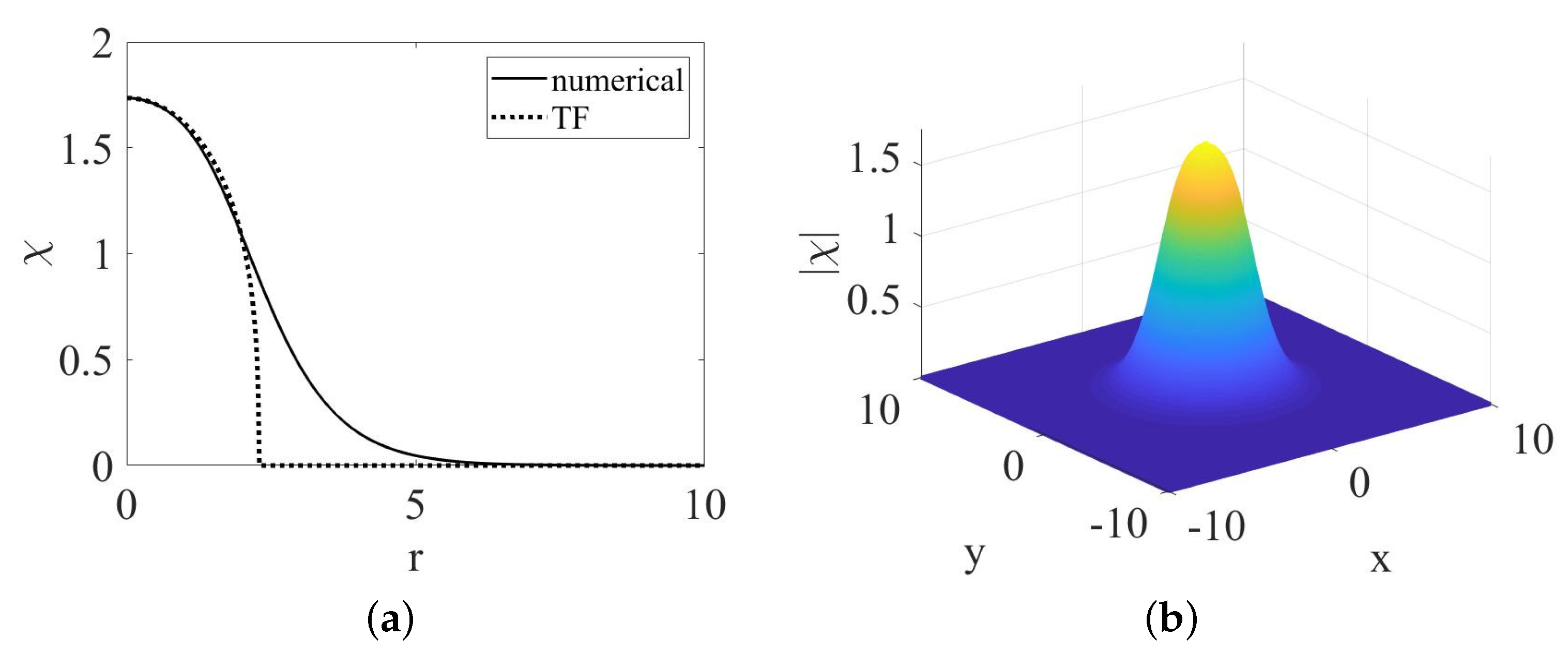
A typical stable GS, obtained as a numerical solution of Equation (30) with , , and , is displayed in Figure 1, together with its counterpart produced by the TF approximation (the interpolation-based approximation, given by Equation (36), is not displayed here, as it is not relevant for large values of ). It is seen that the TF approximation is very close to its numerical counterpart in the inner zone, (see Equation (38)), while in the outer one, , the TF approximation yields zero, being inaccurate, in this sense. Actually, the overall impact of the difference between the numerical and TF solutions in the outer zone is less significant due to the presence of factor in expression (29) for the full solution, . As a result, in the case presented in Figure 1 the relative error of the norm of the TF solution, calculated as per Equation (39), is .
The effect of the MF cubic term of either sign, repulsive () or attractive (), in comparison with the case of , on the GS, is shown in Figure 2. At , all the three shapes converge to a common value, , in agreement with Equation (31).
The counter-intuitive prediction of the existence of the GS in the presence of the repulsive potential in Equation (30), with belonging to interval (33), was also confirmed by the numerical results. Figure 3 displays numerically-found GSs for , taken close to the limit value, , for all the three values of the coefficient in front of the MF cubic term in Equation (30); viz., and . The same figure shows that the interpolating approximation for these solutions, provided by Equation (36), is quite accurate in this case (the TF approximation (38) does not apply to ). It is seen too that the MF cubic term does not strongly affect the solution.
Dependencies for families of the GS solutions, obtained from Equation (30) without and with the repulsive or attractive MF cubic term ( and , respectively), are displayed in Figure 4a,b, for different values of strength of the potential, both and . In panel (a), the curves produced by the TF approximation as per Equation (39) are compared to their numerical counterparts. The same panel demonstrates that the interpolating approximation is very accurate for (while its accuracy is poor for ).
Panel (c) in Figure 4 confirms that, in the presence of the attractive cubic term (), the GS exists at , as predicted by the TF approximation in Equation (43). Up to the accuracy of the numerical results, the threshold value is indeed , as given by Equation (43). This finding is explained by the fact that the width of the GS diverges in the limit of , as seen in Equation (42); hence, in this limit the derivatives become negligible in Equation (26), making the TF approximation asymptotically exact. In principle, must steeply diverge at , according to Equation (44), but it is difficult to collect numerical data very close to the threshold, as the GS is extremely broad in this limit.
The computation of eigenvalues for small perturbations, as well as direct simulations, demonstrate full stability of the GS solutions for both positive and negative values of (at which the GS exists), at all . In particular, Figure 3b demonstrates the stability in the counter-intuitive case of the repulsive potential, with . The stability is not affected by the TF cubic term either, holding for and .
Lastly, the numerical analysis has demonstrated that all vortex modes with (see Equation (25)) are completely unstable, in terms of eigenvalues of small perturbations and direct simulations alike; namely, the spectrum of eigenvalues contains a pair of real ones (see Equation (45). In particular, in direct simulations the instability leads to spontaneous drift of the pivot of the vortex with in an outside direction, along an unwinding spiral trajectory. Eventually, the pivot is ousted to periphery, and the vortex mode transforms into a stable GS with zero vorticity. The norm of the residual GS is essentially smaller than the original value, due to intensive emission of small-amplitude waves in the course of the transient evolution.
3. Singular Solitons in One, Two, and Three Dimensions
This section summarizes original results which were recently reported in [53]. In the 2D case, the results are related to those presented in the previous section for the model with the external potential.
As mentioned in the Introduction, relevant self-defocusing nonlinearities which are necessary to support singular self-trapped states in 3D, 2D, and 1D settings, are represented by the cubic, quintic, or septimal terms, which correspond, respectively, to , 2, and 3 in Equation (10). Realizations of the cubic and quintic nonlinearities of either sign (focusing or defocusing) in diverse physical media are well known [62,63,64,65]. In particular, such nonlinear terms with controllable strengths (including the “exotic” septimal term), can be realized in optical waveguides filled by suspensions of metallic nanoparticles, control parameters being the density and size of the particles [66,67,68].
Results outlined below provide not only solutions in analytical and numerical forms, but also an interpretation of the physical meaning of the singular solitons.
3.1. Analytical Results
3.1.1. The One-Dimensional Model with the Septimal Nonlinearity
Singular solitons created by the 1D version of Equation (10) with the seventh-order defocusing () nonlinearity, , are looked for as
with real function satisfying equation
In the application to the planar optical waveguide, t is not time, but the propagation distance (often denoted z), x is the transverse coordinate, and is the propagation constant.
The asymptotic form of solutions to Equation (47) at does not depend on ,
Note that expression (49) is an exact solution of Equation (47) with , but its integral norm diverges at . For , the exponentially decaying asymptotic form of Equation (48) at is
Lastly, the norm of the 1D soliton family is given by Equation (13),
with the numerical coefficient which is accidentally close to . This dependence satisfies the anti-VK criterion, which, as mentioned above, is necessary for the stability of localized modes supported by repulsive nonlinearities [54].
3.1.2. Physical Interpretation of the 1D Singular Soliton: Screening of a “Bare” -Functional Potential
Although the existence of the stable singular solitons under the action of the septimal self-repulsive nonlinearity is firmly established by the above analysis, this result may seem counter-intuitive, as it is commonly believed that localized modes may only be supported by self-attraction. The purport of the result may be understood by comparing Equation (47) to a modified equation,
which includes an attractive delta-functional potential with strength ; cf. Equation (19). An exact solution to Equation (52) is produced by Equations (20)–(22):
(recall is the amplitude of the mode pinned to the attractive delta-functional potential). The approximate value of the offset in Equation (54) corresponds to the limit of .
This solution may be considered as a regularized version of its singular counterpart (49), which obviously converges to the singular state for . It is also relevant to calculate the value of the Hamiltonian, corresponding to Equation (52),
In the limit of , it is
the negative sign suggesting that solution may be the GS.
A physical interpretation of the ability of the self-repulsive 1D model to create singular solitons is offered by the fact that, according to Equation (54), the strength (“bare charge”) of the delta-functional attractive potential diverges in the limit of , which brings one back to the underlying singular solution given by Equations (49) and (50). This observation implies that an infinitely large “bare attractive charge,” embedded in the self-defocusing septimal medium, is completely screened by the nonlinearity, which builds the singular soliton with the convergent norm, for that purpose. This mechanism roughly resembles the renormalization procedure in quantum electrodynamics, where an infinite bare charge of the electron cancels with other diverging factors, making it possible to produce finite observable predictions.
3.1.3. The Two-Dimensional Model with the Quintic Nonlinearity
In the 2D setting, it is relevant to consider Equation (10) with the quintic self-defocusing term:
In terms of optics, Equation (58) models the paraxial propagation of light in a bulk waveguide, with t being the propagation distance (usually denoted z).
In polar coordinates , solutions of Equation (58) with integer vorticity, , are looked for as
with real amplitude function satisfying the radial equation, cf. Equation (47):
For 2D singular solitons with , Equation (60) produces the following expansion at :
with the respective 2D integral norm converging at . For ,
is an exact solution of Equation (60), but its norm diverges at . The asymptotic form of the solution at is found from the linearized version of Equation (60),
(cf. Equation (50)) where C is a constant, and the second term in the parenthesis is a correction to the lowest approximation.
For vortex states given by Equation (59) with , a singular solution with convergent norm is obtained with the opposite (self-focusing) sign in front of the quintic term in Equation (58), the asymptotic approximation at being
cf. Equation (61). For , Equation (64) represents an exact solution of Equation (60) with the opposite (self-focusing) sign in front of the quintic term, but its integral norm diverges at .
An exact scaling relation for the norm of the solutions, with and alike, follows from Equation (58) with either sign of the quintic term:
(for , a numerically found value is ). This dependence satisfies the anti-VK criterion, ; hence, the respective GS solutions with , maintained by the defocusing quintic nonlinearity, may be (and indeed are) stable, but it contradicts the VK condition per se, ; hence, the vortex states, which exist in the case of self-focusing, are definitely unstable, as corroborated by numerical simulations [53].
3.1.4. Interpretation of the 2D Singular Soliton: Screening of a Ring-Shaped Attractive Potential
Similar to what is outlined above for the 1D model, it is possible to introduce a version of Equation (58) with a delta-functional potential; however, it is concentrated on a ring of a small radius, , instead of the single point. The so modified Equation (60) with is
cf. Equation (52). At , the solution of Equation (66) is sought for in a form similar to that given by Equation (61), while inside the ring it is taken as . Eventually, straightforward manipulations, which take into regard the jump of at , yield a relation between the strength of the delta-functional potential concentrated on the ring and the ring’s radius:
cf. Equation (54). Then, in the limit of , an effective "charge" of the 2D attractive potential is
Thus, the 2D singular soliton may be construed as a solution providing the screening of the finite “charge” by the defocusing quintic nonlinearity.
3.1.5. Effects of Additional Nonlinear Terms on 1D and 2D Singular Solitons
Even if the septimal or quintic term represents the dominant nonlinearity in the underlying NLSE, the lower-order terms, i.e., cubic and/or quintic ones (with respective coefficients and ), should be included in the realistic model of the light propagation [66,67,68]. In particular, the accordingly amended septimal 1D Equation (47) is replaced by
3.1.6. The 3D Model with the Cubic Nonlinearity
In the 3D case, the relevant equation is the NLSE with the usual cubic term:
It has a plethora of physical realizations for both the defocusing () and focusing () signs of the nonlinearity [64], including the GPE for BEC with, respectively, repulsive or attractive interactions between atoms [10]. For isotropic stationary states, , where r is the 3D radial coordinate, the real radial functions obeys the commonly known equation,
For the asymptotic consideration of singular solutions at , the term on the right-hand side of Equation (72) is negligible. Dropping this term and looking for solutions in the form of
where is an arbitary radial scale, one can transform Equation (72) into the following form (which is an exact transformation for :
Formally, Equation (74) is tantamount to the equation of motion of a mechanical unit-mass particle with coordinate and time in the normal () or inverted () quartic potential, , under the action of the friction force with coefficient 1.
For (the focusing nonlinearity), an appropriate asymptotic solution to Equation (74) is one dominated by the balance of the potential and friction forces at , which is relevant for , according to the definition of in Equation (73):
For (defocusing), the appropriate solution to Equation (74) is also determined by the balance of the potential force and friction, the relevant region being ; i.e., :
Both solutions (75) and (76) eventually translate into the asymptotic expression for the 3D density given above by Equation (16).
At the opposite limit of , a straightforward consideration yields an asymptotic expression for the solution in the form of
with constant C; cf. Equation (63).
An exact scaling relation between the 3D norm and chemical potential, as it follows from the cubic NLSE (71), is the same as its counterpart (65) in the 2D model with the quintic nonlinearity:
This relation satisfies the anti-VK criterion; hence, the family of the 3D singular solitons may be (and indeed is) stable in the case of the defocusing cubic nonlinearity, .
3.1.7. Interpretation of the 3D Singular Solitons: Screening of an Attractive Spherical Potential
Similarly to what is presented above for the 2D model, one can augment the 3D model by the attractive delta-functional potential concentrated on a sphere of radius , the respective stationary equation being (cf. Equation (66))
where it is assumed that, although is small, it must be larger than in Equation (73). A stationary solution to Equation (79) is sought for in the form given by Equations (73) and (76) at , and as at . Then, calculations similar to those outlined above in the 2D setting lead to a relation between and the strength of the attractive potential, ; cf. Equation (67). In the limit of (which is imposed along with , so as to keep condition valid), the respective “charge” of the 3D attractive potential is ; cf. Equation (68). Thus, one may realize the 3D singular soliton as a state which provides the screening of the vanishingly small “charge”.
4. Numerical Results for the 1D, 2D, and 3D Singular Solitons
The numerical scheme for producing singular solitons as solutions of the NLSEs with the self-repulsive nonlinearity must be adjusted to the fact that, in the analytical form, the solutions take infinite values at the origin. In [53], a finite-difference scheme was used for this purpose. It was defined on a grid with spacing , constructed so that closest to the origin were points with coordinates
in the 3D case, and similarly in 1D and 2D. At these points, boundary conditions with large but finite values of were fixed according to the asymptotically exact analytical expressions (49), (61), and ( 16).
A typical shape of the 1D singular soliton, produced by exact solution (48) with , is plotted in Figure 5 with step size . In agreement with the fact that the entire family of the 1D singular solitons satisfies the anti-VK criterion, numerical results corroborate the full stability of the family.
In the 2D setting, the numerical solution of the quintic Equation (58) has corroborated the existence and full stability of the singular solitons with zero vorticity (). As an illustration, Figure 6 displays a global view of the stable 2D soliton produced by direct simulations of Equation (58), starting from the initial conditions taken as per exact solution (62) corresponding to (the formal divergence of its integral norm at is restricted by the finite size of the integration domain). In particular, the numerical simulations confirm the stability of the 2D singular solitons against azimuthal perturbations which attempt to break the axial symmetry of the solitons.
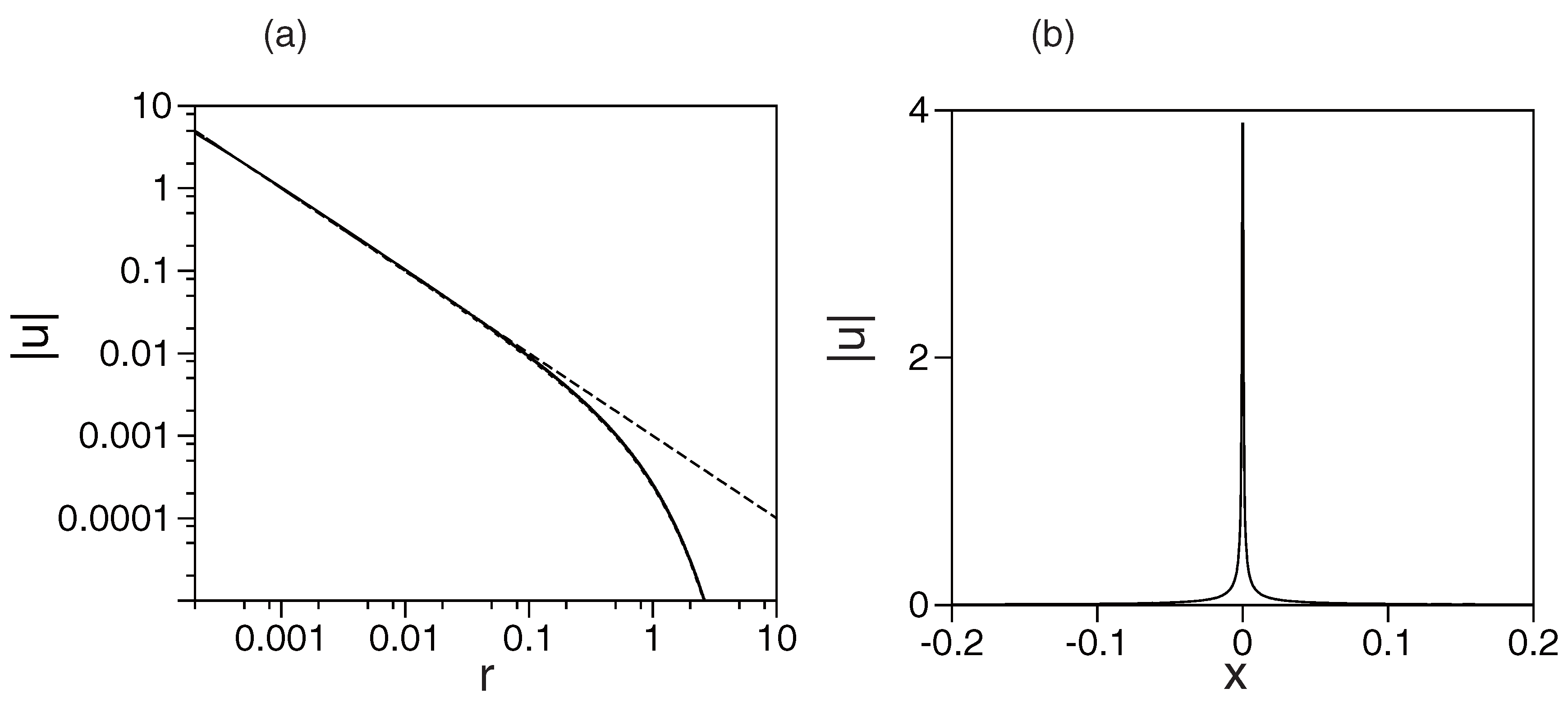
In the 3D setting, the numerical solution of Equation (71) produces a family of 3D singular solitons. A comparison of these solutions with the analytical prediction, given by Equations (73) and (76) for small r, is not straightforward, as the analytical expression contains indefinite parameter . Therefore, an example, displayed in Figure 7a, presents the comparison of the numerical solution to analytical profile at small r, with the constant selected as the best-fit parameter ( for the case of , displayed in Figure 7a).
Further, one can try to use the asymptotic form of the 3D solution at large r, given by Equation (77), with C set equal to the best-fit value of selected at , as a global analytical approximation. Figure 7a demonstrates that such an approximation is extremely close to its numerical counterpart at all values of r.
Finally, direct simulations of the evolution of the 3D singular solitons confirm stability of the soliton family; see an example in Figure 7b.
5. Conclusions
The aim of this paper was to produce a brief review of findings recently reported in works [45,53], which demonstrate the existence of several types of singular bound states in 3D, 2D, and 1D models with self-repulsive nonlinearities. These states feature a singular structure of the density at , while the total norm converges, making the states physically relevant solutions. One model combines the attractive potential in the 2D space and the LHY (quartic) self-repulsive term. The respective GPE (Gross–Pitaevskii equation) is a model of BEC composed of particles carrying permanent electric dipole moments, which are pulled to the central charge. Previously, it was found—in the framework of MF and in many-body quantum settings alike [2,11]—that the quantum collapse, driven by this attractive potential, can be effectively suppressed in the 3D space by the usual cubic nonlinearity (which represents, as usual, repulsive interactions of colliding particles), while the same cubic nonlinearity cannot stabilize the 2D condensate. A brief review of those results was presented in [23].
The new result, reported in [45] and summarized in Section 2 of the present review, is that the quartic self-repulsive term is sufficient to suppress the 2D quantum collapse and restore the missing GS (ground state). An essential peculiarity is that stable 2D modes exist, counter-intuitively, even when the attractive central potential is replaced by the repulsive one, with a sufficiently small strength, as defined by Equation (33). The latter feature is closely related to another topic relevant to the consideration of singular states, which was elaborated in [53] and is summarized in Section 3 of the review. It deals with NLSEs (nonlinear Schrödinger equations) in 1D, 2D, and 3D free space, which contain the septimal, quintic, and cubic repulsive terms, respectively. These equations demonstrate the existence of stable, singular solitons that realize the model’s GS in all the cases, with the 1D solitons having been found in an exact analytical form. The physical interpretation of these counter-intuitive findings is provided by the possibility to construe the singular solitons as a result of screening, by the respective self-repulsive nonlinearity, of a delta-functional attractive potential, whose integral strength is divergent in 1D, finite in 2D, and vanishingly small in 3D.
A common feature of both models considered in this paper is that, contrary to the stable zero-vorticity GSs, two-dimensional vortex states are completely unstable. Therefore, a challenging problem for further work is the search for physically relevant modifications of the 2D models which may allow the existence of stable vortices. A still more challenging objective is to construct 3D states with embedded vorticity and investigate their respective stabilities. Another subject for further work may be singular dissipative solitons in complex Ginzburg–Landau equations [53]. Quite challenging may also be an extension of the analysis for singular modes (if any) in models of Fermi gases based on density-functional equations.
Author Contributions
Conceptualization, B.A.M. and H.S.; Methodology, B.M. and H.S.; Analytical Work, B.M.; Numerical Simulations, H.S., E.S., and Z.C.; Writing—Original Draft Preparation, B.M.; Writing—Review & Editing, B.N.; Project Administration, B.M.; Funding Acquisition, B.M. All authors have read and agreed to the published version of the manuscript.
Funding
This research was funded by Israel Science Foundation: 1286/17.
Acknowledgments
The work on topics relevant to the mini-review was supported, in part, by the Israel Science Foundation through grant number 1286/17.
Conflicts of Interest
The authors declare no conflict of interest.
Abbreviations
The following abbreviations are used in this manuscript:
| 2D | two-dimensional |
| 3D | three-dimensional |
| BEC | Bose–Einstein condensate |
| GPE | Gross-Pitaevskii equation |
| GS | ground state |
| LHY | Lee–Huang–Yang (correction to the mean-field theory) |
| MF | mean field |
| NLSE | nonlinear Schrödinger equation |
| TF | Thomas–Fermi (approximation) |
| VK | Vakhitov–Kolokolov (stability criterion) |
References
- Landau, L.D.; Lifshitz, E.M. Quantum Mechanics: Nonrelativistic Theory; Nauka Publishers: Moscow, Russia, 1974. [Google Scholar]
- Sakaguchi, H.; Malomed, B.A. Suppression of the quantum-mechanical collapse by repulsive interactions in a quantum gas. Phys. Rev. A 2011, 83, 013607. [Google Scholar] [CrossRef] [Green Version]
- Denschlag, J.; Schmiedmayer, J. Scattering a neutral atom from a charged wire. Europhys. Lett. 1997, 38, 405–410. [Google Scholar] [CrossRef]
- Denschlag, J.; Umshaus, G.; Schmiedmayer, J. Probing a singular potential with cold atoms: A neutral atom and a charged wire. Phys. Rev. Lett. 1998, 81, 737. [Google Scholar] [CrossRef]
- Gupta, K.S.; Rajeev, S.G. Renormalization in quantum mechanics. Phys. Rev. D 1993, 48, 5940–5945. [Google Scholar] [CrossRef] [Green Version]
- Camblong, H.E.; Epele, L.N.; Fanchiotti, H.; García Canal, C.A. Renormalization of the Inverse Square Potential. Phys. Rev. Lett. 2000, 85, 1590. [Google Scholar] [CrossRef] [Green Version]
- Camblong, H.E.; Epele, L.N.; Fanchiotti, H.; García Canal, C.A. Dimensional transmutation and dimensional regularization in quantum mechanics: II. rotational invariance. Ann. Phys. (N. Y.) 2001, 287, 57. [Google Scholar] [CrossRef] [Green Version]
- Yafaev, D.R. On a zero-range interaction of a quantum particle with the vacuum. J. Phys. A 1999, 25, 963–978. [Google Scholar] [CrossRef]
- Noja, D.; Posilicano, A. On the point limit of the Pauli-Fierz model. Ann. Inst. Henri Poincaré. 1999, 71, 425–457. [Google Scholar]
- Pitaevskii, L.; Stringari, S. Bose-Einstein Condensation; Clarendon Press: Oxford, UK, 2003. [Google Scholar]
- Astrakharchik, G.E.; Malomed, B.A. Quantum versus mean-field collapse in a many-body system. Phys. Rev. A 2015, 92, 043632. [Google Scholar] [CrossRef] [Green Version]
- Sakaguchi, H.; Malomed, B.A. Suppression of the quantum collapse in an anisotropic gas of dipolar bosons. Phys. Rev. A 2011, 84, 033616. [Google Scholar] [CrossRef]
- Sakaguchi, H.; Malomed, B.A. Suppression of the quantum collapse in binary bosonic gases. Phys. Rev. A 2013, 88, 043638. [Google Scholar] [CrossRef] [Green Version]
- Adhikari, S.K.; Salasnich, L. One-dimensional superfluid Bose-Fermi mixture: Mixing, demixing, and bright solitons. Phys. Rev. A 2007, 76, 023612. [Google Scholar] [CrossRef] [Green Version]
- Bulgac, A. Local-density-functional theory for superfluid fermionic systems: The unitary gas. Phys. Rev. A 2007, 76, 050402. [Google Scholar] [CrossRef] [Green Version]
- Adhikari, S.K. Superfluid Fermi-Fermi mixture: Phase diagram, stability, and soliton formation. Phys. Rev. A 2007, 76, 053609. [Google Scholar] [CrossRef] [Green Version]
- Adhikari, S.K. Nonlinear Schrödinger equation for a superfluid Fermi gas in the BCS-BEC crossover. Phys. Rev. A 2008, 77, 045602. [Google Scholar] [CrossRef] [Green Version]
- Abdullaev, F.K.; Gammal, A.; Tomio, L.; Frederico, T. Stability of trapped Bose-Einstein condensates. Phys. Rev. A 2001, 63, 043604. [Google Scholar] [CrossRef] [Green Version]
- Abdullaev, F.K.; Salerno, M. Gap-Townes solitons and localized excitations in low-dimensional Bose-Einstein condensates in optical lattices. Phys. Rev. A 2005, 72, 033617. [Google Scholar] [CrossRef] [Green Version]
- Burt, E.A.; Ghrist, R.W.; Myatt, C.J.; Holland, M.J.; Cornell, E.A.; Wieman, C.E. Coherence, correlations, and collisions: What one learns about Bose-Einstein condensates from their decay. Phys. Rev. Lett. 1997, 79, 337. [Google Scholar] [CrossRef]
- Stamper-Kurn, D.M.; Andrews, M.R.; Chikkatur, A.P.; Inouye, S.; Miesner, H.J.; Stenger, J.; Ketterle, W. Optical confinement of a Bose-Einstein condensate. Phys. Rev. Lett. 1998, 80, 2027. [Google Scholar] [CrossRef] [Green Version]
- Roberts, J.L.; Claussen, N.R.; Cornish, S.L.; Wieman, C.E. Magnetic field dependence of ultracold inelastic collisions near a Feshbach resonance. Phys. Rev. Lett. 2000, 85, 728. [Google Scholar] [CrossRef] [Green Version]
- Malomed, B.A. Suppression of quantum-mechanical collapse in bosonic gases with intrinsic repulsion: A brief review. Condensed Matter. 2018, 3, 15. [Google Scholar] [CrossRef] [Green Version]
- Petrov, D.S. Quantum mechanical stabilization of a collapsing Bose-Bose mixture. Phys. Rev. Lett. 2015, 115, 155302. [Google Scholar] [CrossRef] [PubMed] [Green Version]
- Petrov, D.S.; Astrakharchik, G.E. Ultradilute low-dimensional liquids. Phys. Rev. Lett. 2016, 117, 100401. [Google Scholar] [CrossRef] [PubMed] [Green Version]
- Żin, P.; Pylak, M.; Wasak, T.; Gajda, M.; Idziaszek, Z. Quantum Bose-Bose droplets at a dimensional crossover. Phys. Rev. A 2018, 98, 051603. [Google Scholar] [CrossRef] [Green Version]
- Ilg, T.; Kumlin, J.; Santos, L.; Petrov, D.S.; Üchler, H.P.B. Dimensional crossover for the beyond-mean-field correction in Bose gases. Phys. Rev. A 2018, 98, 051604. [Google Scholar] [CrossRef] [Green Version]
- Lee, T.D.; Huang, K.; Yang, C.N. Eigenvalues and eigenfunctions of a Bose system of hard spheres and its low-temperature properties. Phys. Rev. 1957, 106, 1135–1145. [Google Scholar] [CrossRef]
- Roy, S.; Landini, M.; Trenkwalder, A.; Semeghini, G.; Spagnolli, G.; Simoni, A.; Fattori, M.; Inguscio, M.; Modugno, G. Test of the universality of the three-body Efimov parameter at narrow Feshbach resonances. Phys. Rev. Lett. 2013, 111, 053202. [Google Scholar] [CrossRef]
- Cabrera, C.; Tanzi, L.; Sanz, J.; Naylor, B.; Thomas, P.; Cheiney, P.; Tarruell, L. Quantum liquid droplets in a mixture of Bose-Einstein condensates. Science 2018, 359, 301–304. [Google Scholar] [CrossRef] [Green Version]
- Cheiney, P.; Cabrera, C.R.; Sanz, J.; Naylor, B.; Tanzi, L.; Tarruell, L. Bright soliton to quantum droplet transition in a mixture of Bose-Einstein condensates. Phys. Rev. Lett. 2018, 120, 135301. [Google Scholar] [CrossRef] [Green Version]
- Semeghini, G.; Ferioli, G.; Masi, L.; Mazzinghi, C.; Wolswijk, L.; Minardi, F.; Modugno, M.; Modugno, G.; Inguscio, M.; Fattori, M. Self-bound quantum droplets of atomic mixtures in free space. Phys. Rev. Lett. 2018, 120, 235301. [Google Scholar] [CrossRef] [Green Version]
- Ferioli, G.; Semeghini, G.; Masi, L.; Giusti, G.; Modugno, G.; Inguscio, M.; Gallemi, A.; Recati, A.; Fattori, M. Collisions of self-bound quantum droplets. Phys. Rev. Lett. 2019, 122, 090401. [Google Scholar] [CrossRef] [PubMed] [Green Version]
- D’Errico, C.; Burchianti, A.; Prevedelli, M.; Salasnich, L.; Ancilotto, F.; Modugno, M.; Minardi, F.; Fort, C. Observation of quantum droplets in a heteronuclear bosonic mixture. Phys. Rev. Res. 2019, 1, 033155. [Google Scholar] [CrossRef] [Green Version]
- Li, Y.; Luo, Z.; Lio, Y.; Chen, Z.; Huang, C.L. Fu, S.; Tan, H.; Malomed, B.A. Two-dimensional solitons and quantum droplets supported by competing self- and cross-interactions in spin-orbit-coupled condensates. New J. Phys. 2017, 19, 113043. [Google Scholar] [CrossRef] [Green Version]
- Li, Y.; Chen, Z.; Luo, Z.; Huang, C.; Tan, H.; Pang, W.; Malomed, B.A. Two-dimensional vortex quantum droplets. Phys. Rev. A 2018, 98, 063602. [Google Scholar] [CrossRef] [Green Version]
- Nilsson Tengstrand, M.; Stürmer, P.; Karabulut, E.Ö.; Reimann, S.M. Rotating binary Bose-Einstein condensates and vortex clusters in quantum droplets. Phys. Rev. Lett. 2019, 123, 160405. [Google Scholar] [CrossRef] [Green Version]
- Kartashov, Y.V.; Malomed, B.A.; Tarruell, L.; Torner, L. Three-dimensional droplets of swirling superfluids. Phys. Rev. A 2018, 98, 013612. [Google Scholar] [CrossRef] [Green Version]
- Kadau, H.; Schmitt, M.; Wentzel, M.; Wink, C.; Maier, T.; Ferrier-Barbut, I.; Pfau, T. Observing the Rosenzweig instability of a quantum ferrofluid. Nature 2016, 530, 194–197. [Google Scholar] [CrossRef]
- Schmitt, M.; Wenzel, M.; Böttcher, F.; Ferrier-Barbut, I.; Pfau, T. Self-bound droplets of a dilute magnetic quantum liquid. Nature 2016, 539, 259–262. [Google Scholar] [CrossRef] [Green Version]
- Ferrier-Barbut, I.; Kadau, H.; Schmitt, M.; Wenzel, M.; Pfau, T. Observation of quantum droplets in a strongly dipolar Bose gas. Phys. Rev. Lett. 2016, 116, 215301. [Google Scholar] [CrossRef]
- Wächtler, F.; Santos, L. Ground-state properties and elementary excitations of quantum droplets in dipolar Bose-Einstein condensates. Phys. Rev. A 2016, 94, 043618. [Google Scholar] [CrossRef] [Green Version]
- Baillie, D.; Blakie, P.B. Droplet crystal ground states of a dipolar Bose gas. Phys. Rev. Lett. 2018, 121, 195301. [Google Scholar] [CrossRef] [PubMed] [Green Version]
- Cidrim, A.; dos Santos, F.E.A.; Henn, E.A.L.; Macrí, T. Vortices in self-bound dipolar droplets. Phys. Rev. A 2018, 98, 023618. [Google Scholar] [CrossRef] [Green Version]
- Shamriz, E.; Chen, Z.; Malomed, B.A. Suppression of the quasi-two-dimensional quantum collapse in the attraction field by the Lee-Huang-Yang effect. to be published.
- Salasnich, L.; Parola, A.; Reatto, L. Effective wave equations for the dynamics of cigar-shaped and disk-shaped Bose condensates. Phys. Rev. A 2002, 65, 043614. [Google Scholar] [CrossRef] [Green Version]
- Muñoz Mateo, A.; Delgado, V. Effective mean-field equations for cigar-shaped and disk-shaped Bose-Einstein condensates. Phys. Rev. A 2008, 77, 013617. [Google Scholar] [CrossRef] [Green Version]
- Jørgensen, N.B.; Bruun, G.M.; Arlt, J.J. Dilute fluid governed by quantum fluctuations. Phys. Rev. Lett. 2018, 121, 173403. [Google Scholar] [CrossRef] [PubMed] [Green Version]
- Bergé, L. Wave collapse in physics: Principles and applications to light and plasma waves. Phys. Rep. 1998, 303, 259–370. [Google Scholar] [CrossRef]
- Veron, L. Singular solutions of some nonlinear elliptic equations. Nonlinear Anal. Theory Methods Appl. 1981, 5, 225–242. [Google Scholar] [CrossRef]
- Lions, P.L. Isolated singularities in semilinear problems. J. Diff. Eq. 1980, 18, 441–450. [Google Scholar] [CrossRef] [Green Version]
- Gidas, B.; Spruck, J. Global and local behavior of positive solutions of nonlinear elliptic equations. Comm. Pure Appl. Math. 1981, 34, 525–581. [Google Scholar] [CrossRef]
- Sakaguchi, H.; Malomed, B.A. Singular solitons. Phys. Rev. E 2020, 101, 012211. [Google Scholar] [CrossRef] [Green Version]
- Sakaguchi, H.; Malomed, B.A. Solitons in combined linear and nonlinear lattice potentials. Phys. Rev. A 2010, 81, 013624. [Google Scholar] [CrossRef] [Green Version]
- Vakhitov, N.G.; Kolokolov, A.A. Stationary solutions of the wave equation in a medium with nonlinearity saturation. Radiophys. Quantum Electron. 1973, 16, 783–789. [Google Scholar] [CrossRef]
- Wang, L.; Malomed, B.A.; Yan, Z. Attraction centers and PT-symmetric delta-functional dipoles in critical and supercritical self-focusing media. Phys. Rev. E 2019, 99, 052206. [Google Scholar] [CrossRef] [PubMed] [Green Version]
- Lam, C.-K.; Malomed, B.A.; Chow, K.W.; Wai, P.K.A. Spatial solitons supported by localized gain in nonlinear optical waveguides. Eur. Phys. J. Spec. Top. 2009, 173, 233–243. [Google Scholar] [CrossRef]
- Tsang, C.H.; Malomed, B.A.; Lam, C.-K.; Chow, K.W. Solitons pinned to hot spots. Eur. Phys. J. D 2010, 59, 81–89. [Google Scholar] [CrossRef]
- Kartashov, Y.V.; Konotop, V.V.; Vysloukh, V.A.; Zezyulin, D.A. Guided modes and symmetry breaking supported by localized gain. In Spontaneous Symmetry Breaking, Self-Trapping, and Josephson Oscillations; Malomed, B.A., Ed.; Springer: Berlin/Heidelberg, Germany, 2013; pp. 167–200. [Google Scholar]
- Malomed, B.A. Spatial solitons supported by localized gain. J. Opt. Soc. Am. B 2014, 31, 2460–2475. [Google Scholar] [CrossRef]
- Yang, J. Nonlinear Waves in Integrable and Nonintegrable Systems; SIAM: Philadelphia, PA, USA, 2010. [Google Scholar]
- Quiroga-Texeiro, M.; Michinel, H. Stable azimuthal stationary state in quintic nonlinear optical media. J. Opt. Soc. Am. B 1997, 14, 2004–2009. [Google Scholar] [CrossRef]
- Boudebs, G.; Cherukulappurath, S.; Leblond, H.; Troles, J.; Smektala, F.; Sanchez, F. Experimental and theoretical study of higher-order nonlinearities in chalcogenide glasses. Opt. Commun. 2003, 219, 427–433. [Google Scholar] [CrossRef] [Green Version]
- Malomed, B.A.; Mihalache, D.; Wise, F.; Torner, L. Spatiotemporal optical solitons. J. Opt. B Quant. Semicl. Opt. 2005, 7, R53–R72. [Google Scholar] [CrossRef]
- Falcão-Filho, L.E.; de Araújo, C.B.; Boudebs, G.; Leblond, H.; Skarka, V. Robust two-dimensional spatial solitons in liquid carbon disulfide. Phys. Rev. Lett. 2013, 110, 013901. [Google Scholar] [CrossRef] [Green Version]
- Reyna, A.S.; de Araújo, C.B. Spatial phase modulation due to quintic and septic nonlinearities in metal colloids. Opt. Exp. 2014, 22, 22456–22469. [Google Scholar] [CrossRef] [PubMed]
- Reyna, A.S.; Jorge, K.C.; de Araújo, C.B. Two-dimensional solitons in a quintic-septimal medium. Phys. Rev. A 2014, 90, 063835. [Google Scholar] [CrossRef]
- Reyna, A.S.; de Araújo, C.B. High-order optical nonlinearities in plasmonic nanocomposites —-A review. Adv. Opt. Photon. 2017, 9, 720–774. [Google Scholar] [CrossRef]
Figure 1.
(a) The profile of a (stable) numerically-found ground state (GS) and its TF counterpart, produced by Equations (30) and (38), respectively, for , , and . The norms of the numerical and approximate solutions are , . (b) The global view of the numerical solution.

Figure 2.
Numerically generated stable GS solutions of Equation (30) for ; and , 0, and . The respective norms are , , and .
Figure 2.
Numerically generated stable GS solutions of Equation (30) for ; and , 0, and . The respective norms are , , and .
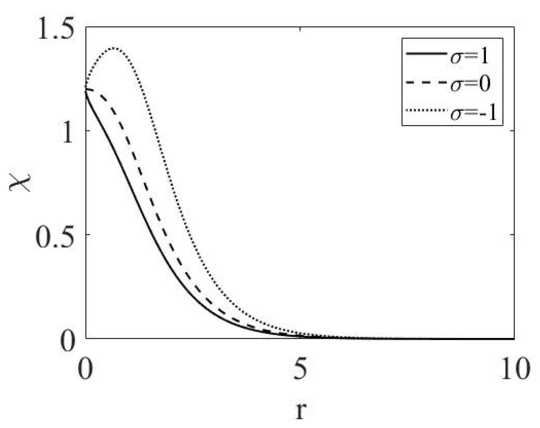
Figure 3.
(a) Radial profiles of numerically-found GSs, produced by Equation (30), and the respective interpolation profile (36), in the presence of the repulsive potential in Equation (30), with , at , without and with the repulsive or attractive mean-field (MF) cubic term ( and or , respectively). The corresponding values of the norm are , , and . The interpolating approximation gives , as per Equation (37). (b) Stability of the GS mode in direct simulations, in the case of .
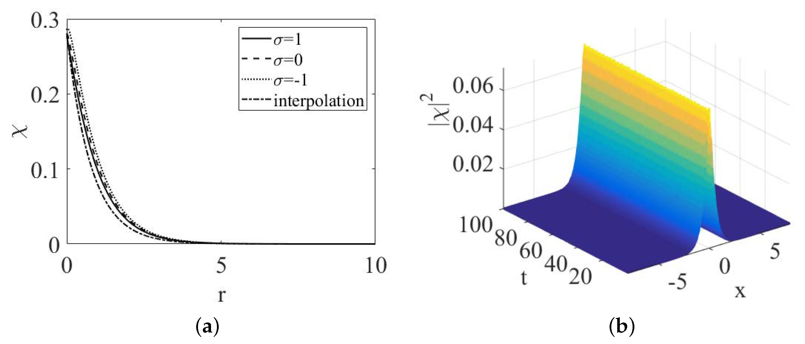
Figure 4.
Dependencies for stable GS solutions with , and for , , , which correspond, respectively, to the repulsive and attractive central potential (in the former case, N is multiplied by 10, as the actual values of the norm are too small in this case). Panels (a) and (b) correspond to the system which does not or does include the repulsive or attractive cubic term ( and , respectively). In (a), the numerical results are juxtaposed with the TF counterparts produced by Equation (39) (except for , when the TF approximation is irrelevant; however, in this case the interpolating approximation, based on Equation (37), is very close to the numerically generated curve). In (b), the numerical curves are compared for and . Panel (c) is a zoomed-in view of the plot from (b) at small values of , with the aim of showing relative proximity to the threshold value for , as predicted in the TF approximation by Equation (43) (this point is discussed in detail in the text).
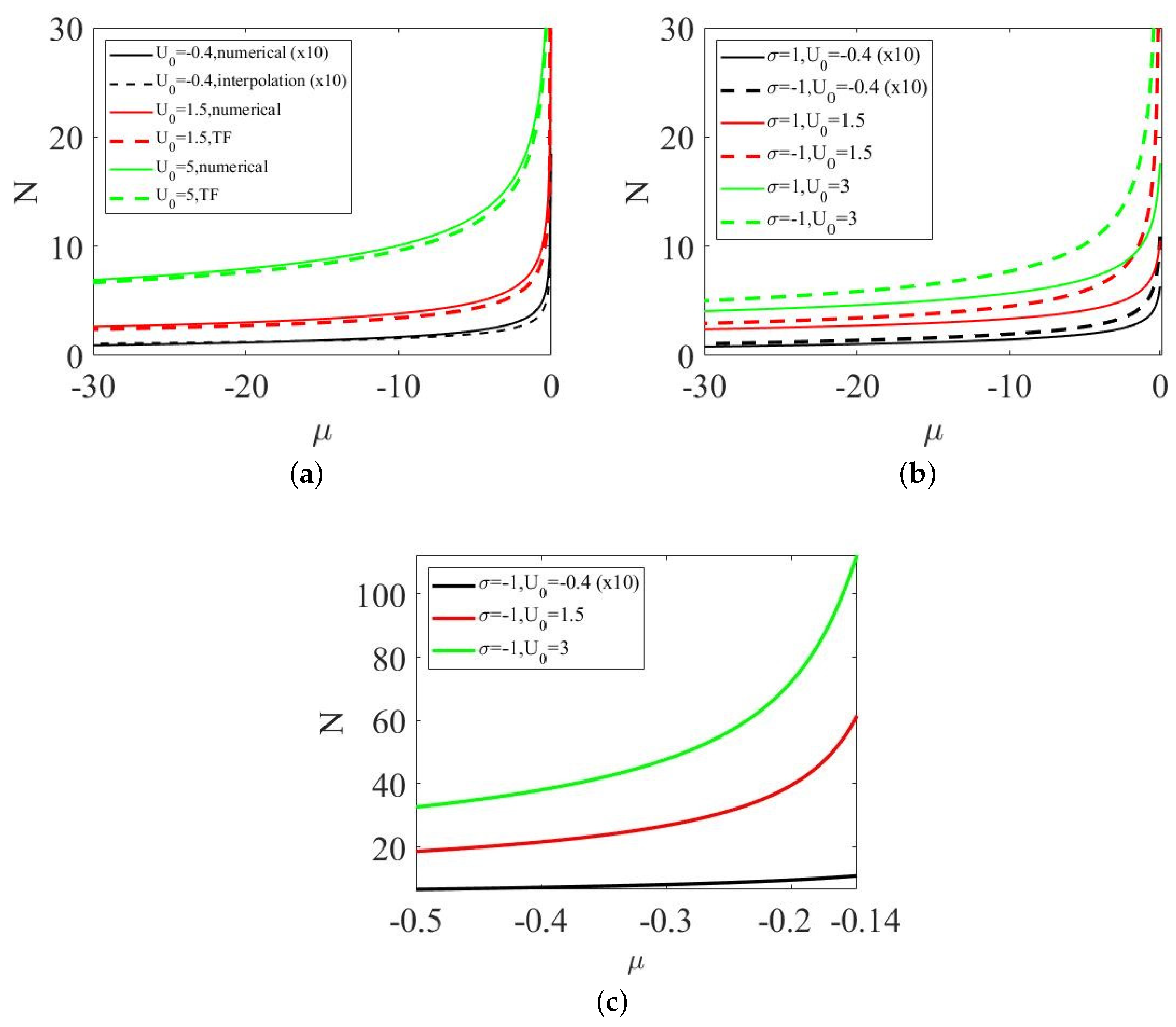
Figure 5.
The shape of the singular 1D soliton, as given by Equation (48) with .
Figure 5.
The shape of the singular 1D soliton, as given by Equation (48) with .
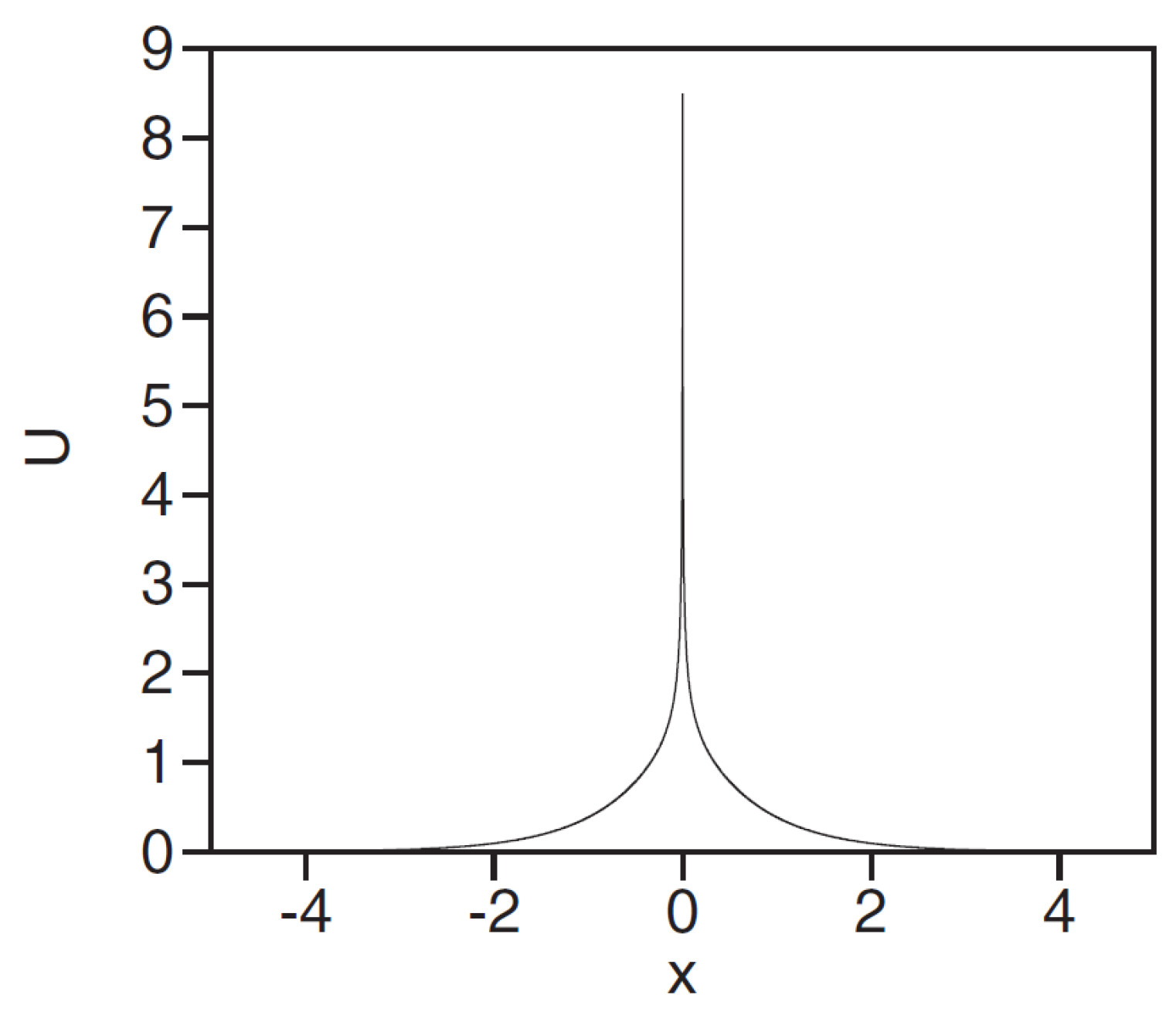
Figure 6.
A stable 2D singular soliton produced by simulation of the full 2D Equation (58), starting from input (62).
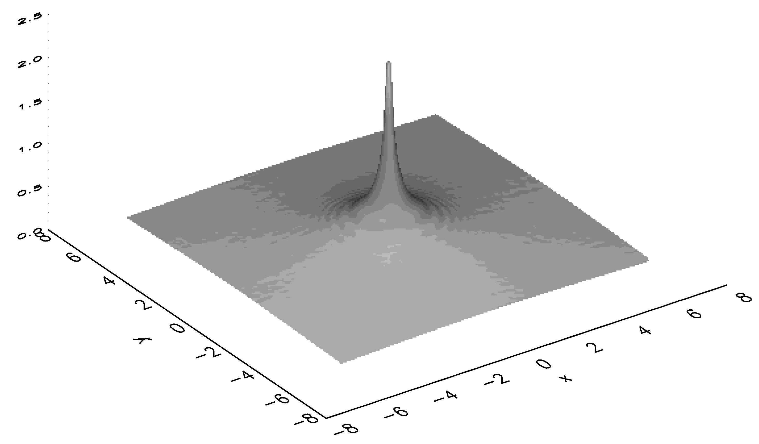
Figure 7.
(a) The comparison, on the double-logarithmic scale, of the numerically found stationary solution of Equation (71) for the 3D singular soliton with (the continuous line) with profile relevant at small r (the long-dashed line), and the global approximation provided by Equation (77) with (the short-dashed line); see explanation in the text. The difference between the latter analytical approximation and the numerical solution is barely visible. (b) The radial cross section of the 3D singular soliton, produced at by direct simulations of Equation (71), with the input taken from panel (a). The result confirms the stability of the 3D singular soliton. In this figure, labels for and are replaced by .

© 2020 by the authors. Licensee MDPI, Basel, Switzerland. This article is an open access article distributed under the terms and conditions of the Creative Commons Attribution (CC BY) license (http://creativecommons.org/licenses/by/4.0/).
Share and Cite
MDPI and ACS Style
Shamriz, E.; Chen, Z.; Malomed, B.A.; Sakaguchi, H. Singular Mean-Field States: A Brief Review of Recent Results. Condens. Matter 2020, 5, 20. https://doi.org/10.3390/condmat5010020
AMA Style
Shamriz E, Chen Z, Malomed BA, Sakaguchi H. Singular Mean-Field States: A Brief Review of Recent Results. Condensed Matter. 2020; 5(1):20. https://doi.org/10.3390/condmat5010020
Chicago/Turabian StyleShamriz, Elad, Zhaopin Chen, Boris A. Malomed, and Hidetsugu Sakaguchi. 2020. "Singular Mean-Field States: A Brief Review of Recent Results" Condensed Matter 5, no. 1: 20. https://doi.org/10.3390/condmat5010020