Article

PedNet: A Spatio-Temporal Deep Convolutional Neural Network for Pedestrian Segmentation

Department of Computer Science, Norwegian University of Science and Technology, 2815 Gjøvik, Norway
*
Author to whom correspondence should be addressed.
J. Imaging 2018, 4(9), 107; https://doi.org/10.3390/jimaging4090107
Submission received: 13 July 2018 / Revised: 22 August 2018 / Accepted: 28 August 2018 / Published: 4 September 2018

Abstract

:
Articulation modeling, feature extraction, and classification are the important components of pedestrian segmentation. Usually, these components are modeled independently from each other and then combined in a sequential way. However, this approach is prone to poor segmentation if any individual component is weakly designed. To cope with this problem, we proposed a spatio-temporal convolutional neural network named PedNet which exploits temporal information for spatial segmentation. The backbone of the PedNet consists of an encoder–decoder network for downsampling and upsampling the feature maps, respectively. The input to the network is a set of three frames and the output is a binary mask of the segmented regions in the middle frame. Irrespective of classical deep models where the convolution layers are followed by a fully connected layer for classification, PedNet is a Fully Convolutional Network (FCN). It is trained end-to-end and the segmentation is achieved without the need of any pre- or post-processing. The main characteristic of PedNet is its unique design where it performs segmentation on a frame-by-frame basis but it uses the temporal information from the previous and the future frame for segmenting the pedestrian in the current frame. Moreover, to combine the low-level features with the high-level semantic information learned by the deeper layers, we used long-skip connections from the encoder to decoder network and concatenate the output of low-level layers with the higher level layers. This approach helps to get segmentation map with sharp boundaries. To show the potential benefits of temporal information, we also visualized different layers of the network. The visualization showed that the network learned different information from the consecutive frames and then combined the information optimally to segment the middle frame. We evaluated our approach on eight challenging datasets where humans are involved in different activities with severe articulation (football, road crossing, surveillance). The most common CamVid dataset which is used for calculating the performance of the segmentation algorithm is evaluated against seven state-of-the-art methods. The performance is shown on precision/recall, F 1 , F 2 , and mIoU. The qualitative and quantitative results show that PedNet achieves promising results against state-of-the-art methods with substantial improvement in terms of all the performance metrics.

1. Introduction

Segmentation is an active field of research in computer vision community and it has wide range of applications including video surveillance [1], crowd analysis [2], robot navigation [3], object recognition [4], medical imaging [5], and human behavior analysis [6]. In fact, segmentation is the equivalent of human perceptual grouping where human vision system groups high-level semantics (shape, geometry, and object category) from low-level information (color, texture, and edge). The perceptual grouping is easy for human and it is carried out on daily basis. However, for a computer, it is a very complex and challenging task.
Segmentation can be carried out either in a supervised or in an unsupervised fashion. The former approach consists of feature extraction followed by a classification module where either image patch or image pixels are classified into different classes. In the latter approach, segmentation is performed in terms of perceptual grouping which is commonly known as clustering. In general, supervised approaches for segmentation can be classified into traditional hand-crafted feature based and more recent deep learning based approaches which train a deep network on manually annotated data. During training, the network parameters are optimized and then pixel-wise segmentation is performed on the test images. Usually, segmentation is performed on a per image/frame basis. However, if the aim is to segment a sequence of frames, due to temporal continuity, there is meaningful temporal information that could be exploited. Some of the video features that change frame to frame are the viewpoint, scale of pedestrian, background, and illumination. If these factors are not model properly, it can deteriorate the performance of segmentation to a great extent. Unfortunately, techniques that reply on a single-frame for segmentation don’t get the perspective knowledge of the scene and have no mechanism for modeling these attributes of a video. However, by exploiting the continuity of video signal, these problems could be addressed. Inspired by this idea, our proposed PedNet segments a frame in a supervised fashion considering both past and future frames. The design of our network exploits temporal information for spatial segmentation. To the best of our knowledge, our PedNet is the first deep FCN that incorporates temporal information for spatial per-pixel segmentation and trains the model end-to-end from scratch. Moreover, compared to standard approaches where computational intensive pre- or post-processing is performed to enhance the segmentation mask, our network does not rely on any pre- or post-processing modules such as super-pixels [7,8], region proposal generation [9], post-hoc refinement through random fields or discriminative classifiers [7,8].
Our proposed PedNet consists of a single mutually combined encoder–decoder network. Generally, the lower layers in a deep network learn low-level features like edges, curves, and semi-circles. The deeper layers learn high-level semantic information. For segmentation, both pieces of information are very useful since high-level semantic information helps to localize and differentiate between the pedestrian and background. The low-level information helps to draw sharp and high-resolution boundaries between the pedestrian and the background. The encoder network in PedNet is responsible for extracting low-level features and the decoder network learns high-level semantic information. The long-skip and feature map concatenation from the encoder to the decoder network combines the low-level fine-grained features learned by the encoder network with the high-level semantic information learned by the decoder network. As a result, better segmentation with sharp boundaries is achieved.
Our PedNet is inspired from U-net [5] that introduced the long-skip connections and was used for medical images segmentation specifically, cell segmentation in microscopy images. Compared to U-net, our architecture has the following differences.
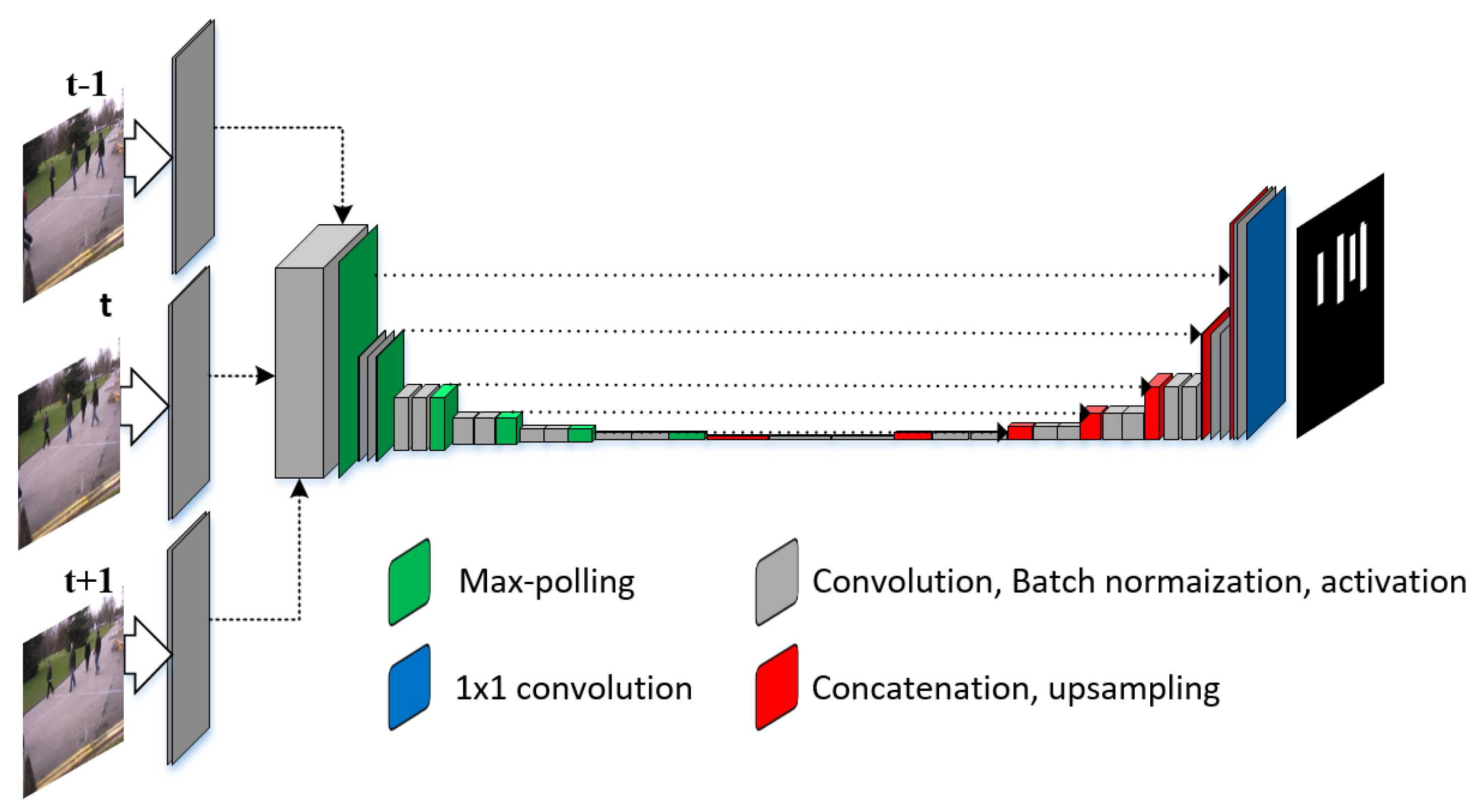
  • Instead of a single input frame, our network takes three frames as input and exploits the temporal information for spatial segmentation.
  • Our proposed PedNet is deeper and we fixed the size of convolution filter to 3 × 3 and a fixed max-pooling window size of 2 × 2 throughout the network. We tested ReLu and SeLu activation functions and used batch normalization after every convolution layer.
  • The network is trained from scratch and data augmentation strategies are adopted which enables the network to train on a limited amount of data.
Our PedNet network is generic and can be used for any computer vision application having a sequence of frames including medical imaging and video surveillance. The rest of the paper is organized in the following order. Section 2 briefly explains the related work in the literature. The overview of the proposed method is presented in Section 3. The architecture of the model is elaborated in Section 4. Training strategy, the objective function, and data augmentations are explained in Section 5. Quantitative results are provided in Section 6. Network analysis and future directions are discussed in Section 7 and the paper is concluded in Section 8.

2. Related Work

In a nutshell, segmentation techniques can be classified into two broad categories i.e., traditional approaches using hand engineered features and deep learning based approaches. Usually, traditional approaches use a multi-stage pipeline that is inefficient, slow, and inelegant. The usual steps in the pipeline are pre-processing, feature extraction, a classification module, and post-processing. For post-processing, a conditional random field is used that refines the segmentation result. Most often, each step of the pipeline is designed independently and there is very little coherency between different step. Compared to traditional approaches, deep learning based methods design a framework for segmentation where features are learned from the data and all the steps work in a hierarchical fashion in a consistent and coherent way. The training of deep models are done end-to-end and it gives better performance with a large margin compared to techniques relying on hand-crafted features. In the following, a brief overview is given for each approach.

2.1. Hand-Crafted Feature Based Segmentation

In such approaches, first features are extracted from an image or a patch of image through a pre-defined rule (color histogram, gradient histogram, local binary pattern) and then it is fed to a classifier, e.g., SVM, boosting [10,11] or random forest [12,13] to calculate the class probability of the patch or whole image. For example, Sturgess et al. [10] use appearance and motion features (textons, color, location and HoG [14]) in a probabilistic CRF model for segmentation. They used a boosting approach to constructively combine the appearance and motion cues. Moreover, higher-order potentials are incorporated in the CRF model for accurate boundary delineation in the segmentation map. Jamie et al. [12] introduced a low-level feature descriptor named as semantic texton forest (STF) for segmentation. Technically, STF is an ensemble of randomized decision forest and use simple pixel comparisons on whole image or image patch for the classification of patch category. Lubor et al. [11] come up with a probabilistic model and defined a single energy function which combines cues from a sliding window object detector and low-level pixel values for segmentation. Yang et al. [15] introduced local label descriptor for segmentation. Local label descriptor is a histogram which is acquired by concatenating pixel label over a fixed size cell in an image patch. They applied sparse coding [16] on the descriptor for introducing sparsity and used the random forest for patch classification. Kontschieder et al. [17] exploited structural feature for segmentation. Structural feature refers to the topological distribution of different object classes in an image. It is inspired by the fact that different object form a coherent region in an image and it is not randomly dispersed in the image. Moreover, they used a classical random forest classifier but modify it according to the structural information. By exploiting the depth information, Chenxi et al. [18] use a dense depth map for the segmentation. They extracted five features (surface normal, height above ground, surface local planarity, surface neighboring planarity, and distance to camera path) from the depth maps and used the random forest for the classification. Similarly, Xiaofeng et al. [19] combined RGB-D feature with kernel descriptor (gradient, color, local binary pattern, depth gradient, surface normal, and Kernel principal component analysis [20]) to generate super-pixel and used a linear SVM for super-pixel classification.
Techniques based on hand-crafted features were quite popular for segmentation until the breakthrough work of Krizhevsky et al. [21] for image classification. Inspired by his work, many deep learning based techniques were introduced in the last couple of years. They become the method of choice for segmentation because, generally, they outperform the traditional hand-crafted features based approaches by a large margin. In the following, the most prominent deep learning-based techniques for segmentation are briefly explained.

2.2. Deep Learning Based Segmentation

A hierarchical architectural model where features are learned from the data is referred to as a deep learning model. There are a variety of model for different applications; from image classification [4,21,22,23,24], image segmentation [25,26,27] to speech processing [28,29]. In such approaches, rather than extracting features from an image or image patch by a pre-defined rule, convolution filters are learned from the data to get the features. For image segmentation, the most suitable deep learning model is a feed-forward Fully Convolutional Network (FCN) [5,30]. It is because FCN can be trained end-to-end, pixels-to-pixels which is an essential part of pixel-wise segmentation. Moreover, segmentation based on FCN can take the whole image as an input and perform agile and precise pixel inference. Architectural wise, FCN is a special convolutional neural network which doesn’t have any fully connected layers. In connection with FCN, Long et al. [31] introduced a fully convolutional neural network for semantic segmentation. The backbone of their architecture relies on standard image classification networks like [4,21,22] and fine-tuned it without the fully connected layers for the segmentation. Similarly, Badrinarayana et al. [25] came up with a deep architecture where they used the first 13 layers of pre-trained VGG net [22] as an encoder for reducing the resolution of feature maps and a similar architecture as a decoder for up-sampling the feature maps. Different from [5,31], Badrinarayana et al. [25] uses fully connected layers at the end of the network for pixel classification. Noh et al. [30] used a similar approach as [25,31] and used a pre-trained VGG network [22] for downsampling and corresponding network for upsampling but they did not use any long skip connections. Their architecture works in a sequential way where the input goes at one end and processing is done step by step in a hierarchical fashion and generate the segmentation mask at the output. Moreover, they also didn’t use any fully connected layer for the pixel-wise classification. Chen et al. [26,32] explored Atrous Convolution (AC) and Atrous Spatial Pyramid Pooling (ASPP) in a Deep Convolutional Neural Network (DCNN) for segmentation at multi-scale. To improve boundary delineation and localization accuracy, they combined the output of DCNN with a fully connected conditional random field. Lin et al. [27] used a similar architecture [31] but instead of max-pooling, they introduced chained residual pooling which enables the network to capture the background context from a large image region. It downsamples the feature maps at multiple window sizes and then combines with the low-level feature maps through long-skip connections. Zanjani and Gerven [33] tried to use temporal information and proposed a hybrid approach for pixel-wise segmentation. Initially, they used a well define convolutional neural network i.e., Deeplab [26] to get the pixel-wise segmentation. In the second step, a spatial CRF model is used as a post-processing for refining the segmentation results. The CRF model use scene appearance and dense optical flow information for inference. Hence, they incorporate temporal information as a post processing for segmentation. Shelhamer et al. [34] focused on the execution time of a CNN and tried to exploit the temporal continuity of a video for faster network execution. They introduced clockwork CNN where different layers of CNN are connected to a clock signal. The argument is, even though, a scene changes from frame to frame but the semantic content of the scene changes slowly. Given that different layers of a CNN learns different features (from low-level to high-level semantic information), hence, the feature maps that learn high-level semantic information should change slowly as the video is processed from one frame to the next frame. Luc et al. [35] trained an autoregressive convolutional neural network named S2S model for predicting the semantic segmentation maps of the future frames. The input to the network is segmentation maps of N previous frames and the network predict the segmentation map of the future frames. In essence, the network learns the pattern of the segmentation maps of the previous frames and based on the previous results, predict the segmentation map of the future frames without seeing the RGB frame. In this setup, the predicted segmentation mask of the future maps shows convincing results until half a second.

3. Proposed PedNet Overview

The architecture of our network is given in Figure 1. The input to the network is set of three frames and output is a binary mask. After the first convolution in the encoder network, the resolution of feature maps keep reducing but the number keeps increasing. The network learns to incorporate temporal information from t 1 and t + 1 frame in such a way that it gives optimal segmentation for the middle frame. In the decoder network, rather than adding the feature maps, we concatenate it so that every feature map contribution in the segmentation. At the end of the network, a 1 × 1 convolution is applied that gives a single binary mask. The binary mask is processed to highlight the pedestrian in the original frame Figure 2. The details of the architecture are given in Section 4. It is important to note that we have only 3979 samples for training the network. These are collected from 8 datasets Section 6.1 and manually annotated to highlight the pedestrian and the background. To increase the size of the dataset, we applied data augmentation Section 5.2 strategies which not only handle the problem of under-fitting but also enhance the generalization ability of the network. Moreover, extensive experiments are conducted on a variety of datasets (sports, surveillance, and traffic) to validate the performance of our network. In the following sections, each step of the proposed PedNet is explained in details.

4. PedNet Architecture

The network architecture is illustrated in Figure 1. The structure of PedNet is symmetric and has an encoder network with a corresponding decoder network. In the context of deep architecture, resolution reduction of the feature maps is done by the encoder network through a subsequent 2 × 2 max-pooling layers that are followed by every convolution step in encoder network. Similarly, an increase in the resolution of feature maps is reflected by the decoder network. The structure of encoder and decoder network follows a classical architecture of feed-forward convolutional neural network similar to [4,21,22,23,24]. However, unlike these models, we have long skip connections which transfer the feature maps from the encoder network to the decoder network. The encoder network consists of 17 convolution layers, each followed by downsampling. The size of the convolution filter is fixed to 3 × 3 and each convolution is followed by a rectified linear unit (ReLU) and a 2 × 2 max pooling operation with stride 2 for downsampling. We also tried Self-Normalizing linear unit (SeLU) instead of ReLU but the performance was not affected. At each downsampling step, the resolution of the feature map decreases but the number of feature channels increases. Every step in the decoder network consists of an upsampling of the feature map, a concatenation with the corresponding feature map from the encoder network (long-skip), and two 3 × 3 convolutions, each followed by a ReLU. Hence, the decoder network reduces the number of feature channels but increase the resolution of feature maps. The complete architecture and details about each layer are given in Table 1.

5. Network Training

We labeled our training data such that for each image, we generated a binary mask where the white regions correspond to the pedestrian and the black region corresponds to the background. The binary masks and its corresponding original frame makes a single sample of the training set. The batch size was set to 7 (7 × 3 = 21 frames and corresponding masks) and stochastic gradient descent is used to train the network end-to-end. Classical stochastic gradient descent has three problems i.e., it is slow, often get stuck in the local minima and has an oscillatory behavior while converging to the solution. To address these issues, we used RMSprop [41] while updating the hyper-parameters of the networks. The update of the parameters is done by introducing intermediate parameters I d b , and I d w which are also known as the running average of the squared gradients.
Let us assume at iteration t, we compute the derivative of the parameter w as d w (convolutions filters) and b (bias) as d b using stochastic gradient descent on the current batch. Then, the intermediate terms are calculated as:
I d w t = γ I d w t 1 + ( 1 γ ) d w t 2
and
I d b t = γ I d b t 1 + ( 1 γ ) d b t 2
Once the intermediate terms are calculated, the main parameters are updated according to the following:
w t + 1 = w t η d w t I d w t + ε
and
b t + 1 = b t η d b t I d b t + ε
For the numeric stability, a small number ε is added in the denominator of both terms to avoid division by zero. The learning rate η is chosen to be 10 4 while the γ is set to 0.9 . With RMSprop, we can also use bigger learning rate without the fear of divergence as the intermediate terms I d b and I d w keeps the update in control.

5.1. Objective Function

Compared to the state-of-the-art techniques [5,30,31] where they usually use a pre-trained VGG network [24], we designed our own network and initialized the parameters using the strategy of [42]. The input to our network is a set of three frames at three different time instants i.e., t 1 , t and t + 1 . Segmentation is performed for the frame at time instant t. The frames at time instant t 1 and t + 1 only provide temporal information and assist the segmentation. The output of our decoder network is a single channel binary mask of the frame at time instant t where pixels correspond to the pedestrians are marked white. The loss of the network is defined by applying convolution with sigmoid activation. Let us assume that P is the predicted mask and G is the groundtruth, the binary cross entropy, and dice coefficient loss between the two binary images is calculated as the following:
L ( P , G ) = 1 N i = 1 N ( λ 2 . g i . log p i ) + 1 2 i = 1 N ( g i . p i ) + ϵ i = 1 N p i + i = 1 N g i + ϵ
where λ and ϵ are false negatives (FN) penalty and smoothing factor, respectively. The first term in Equation (5) penalizes false negative (FN) and the second term weights false positive (FP) and false negative (FN) equally. In other words, the second term is the same as the negative of F 1 -score. This is to avoid miss detection (false positive) of the pedestrian. We give more weight to miss a pedestrian than giving a FP. Hence, the summed loss function gives a good balance between FN and FP.

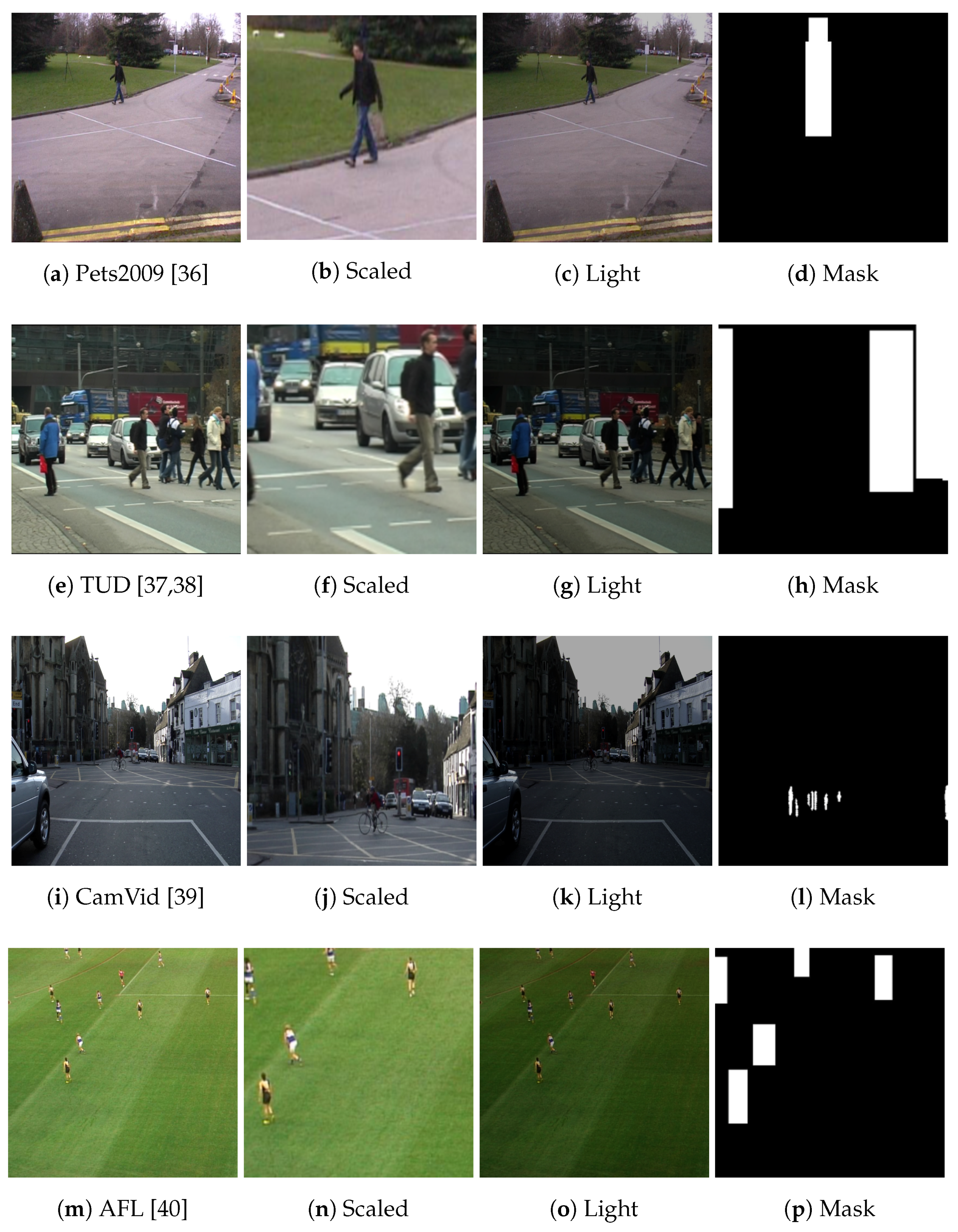
5.2. Data Augmentation

The purpose of an FCN is to approximate a function from the training data through inductive learning. The approximated function should map the input variables to the output variable. In our case, the input is the set of three frames and the output is a binary mask of the central frame. A crucial aspect of learning is how well the learned model generalizes to the new data. Generalization is essential because the training data that we labeled is only a partial portrait of the original test data that the machine will actually segment. When the training data is small, generalization is difficult to achieve and there is the problem of under-fitting. To increase the training data, one possible approach is to generate the data synthetically. However, in our case, it needs sophisticated 3D modeling of the pedestrian which is beyond the scope of this paper. Instead of 3D modeling, we adopted data augmentation strategies. Data augmentation is crucial because it teaches the network the desired invariance and robustness properties in a customized fashion. Different data augmentations are possible like rotation, scaling, robustness to deformation and gray value variations. In the case of pedestrians, the rotation is not relevant as pedestrian usually follow a linear motion and in most cases, the shape remains rotation invariant. We used scaling and light intensity variation for augmenting the data Figure 3. Both types of augmentation are performed randomly. Roughly, 50% of the training samples are used without any augmentation. In the remaining 50%, scaling and light intensity variation is introduced. For scaling, we crop the region in a frame. While for the light intensity variation, we first introduced a Gaussian noise with zero means and unit standard deviation. After that, gamma correction is applied for varying the gray level values. The samples of original frames and its augmented versions are shown in Figure 4.

6. Experiment

This section first explains the datasets that we used for evaluating our PedNet. Second, features learned by the network are visualized and the effectiveness of temporal information is argued. For visualization, Grad-CAM [43] is used. Third, the implementation details are briefly reviewed. And in the last, the performance metric that is used for quantitative analysis are discussed and results are shown against state-of-art methods. Quantitative results of PedNet are given in Table 2 and Table 3.

6.1. Datasets

We quantify the performance of PedNet on 8 datasets that are most commonly used for segmentation and tracking. The first is Cambridge-driving Labeled Video Database (CamVid) [39] that is recorded from driving automobile. It is recorded with a frame rate of 30 and consist of 702 frames in total. As the automobile moves, the heterogeneity of the observed classes changes. However, our focus is only segmenting the pedestrians. Similarly, Pets2009 is a video surveillance dataset and commonly used for evaluating tracking algorithms. It has three views and recorded at a university campus. At most, ten people move in the scene. There are a total of 795 frames in each view and it is recorded at a low frame rate of 7 fps. Like Pets2009, TUD also has three variant (crossing, campus, stadmitt). It is recorded from a short distance and the pedestrian comparatively looks big. We also included a dataset from sports (AFL). In the scene, the players look considerably small and the maximum number of the players changes from 10 to 20. The visual results can be seen in Figure 2.

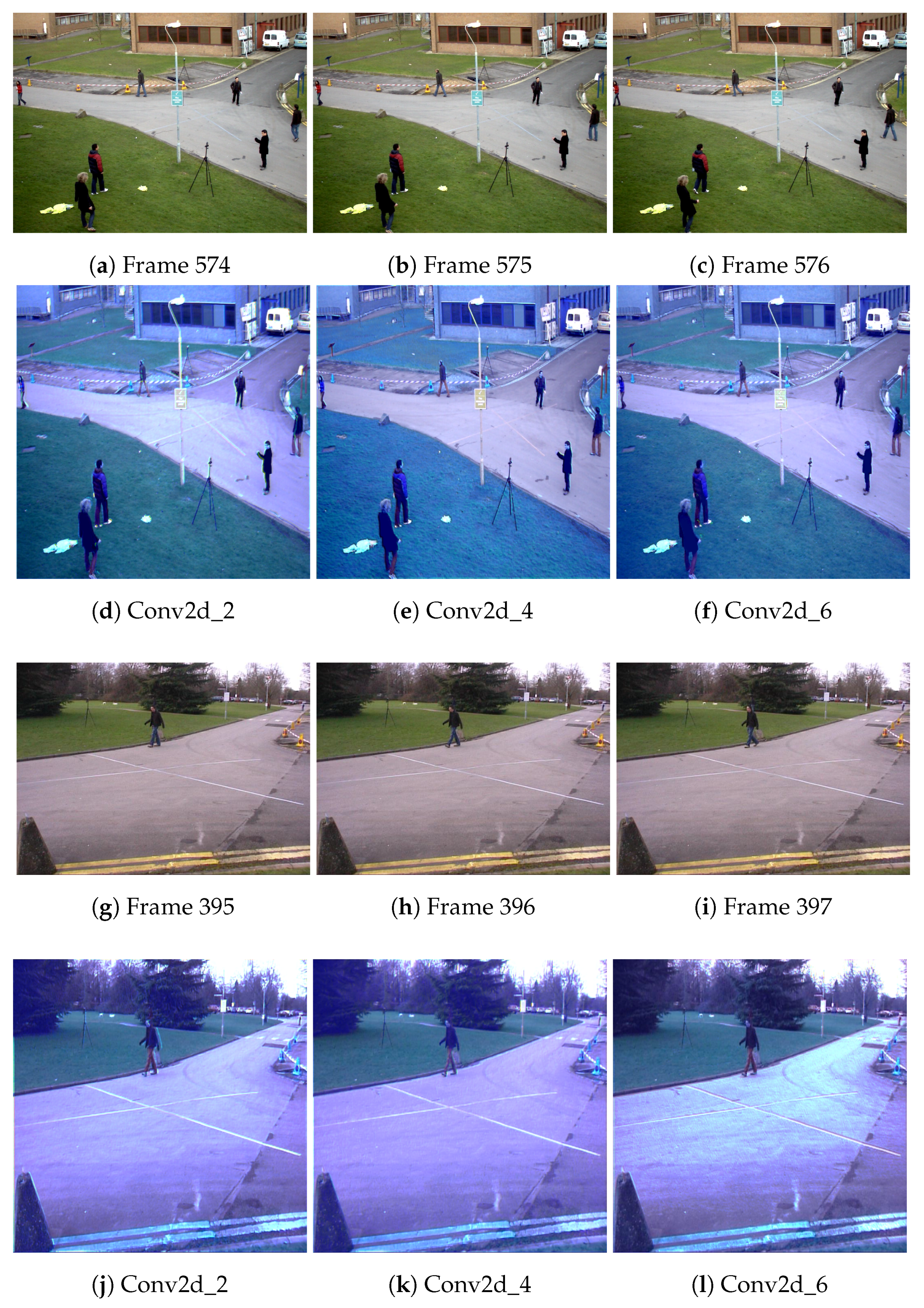
6.2. Feature Visualization

To justify our claim regarding the temporal information, we visualized the activation of different layers of the network. Technically, the layers of the network should learn different information in order to extract discriminative features from each frame. We focused mainly on the convolution layers Conv2d_2, Conv2d_4, and Conv2d_6. It is because these are the first convolutions in the encoder network. After these convolutions, the feature maps are fused and it is not possible to differentiate the frames at t 1 , t, and t + 1 . We used Grad-CAM [43] to get the maximum activation of the layer. In Figure 5d,j corresponds to the activation of frame at t 1 . Similarly, Figure 5e,k gives the activation at time t and Figure 5f,l is related to activation at t 1 . It is obvious from the figures that the activations are different from each other. Especially, the RGB value response is different which is also proved by [22] that the first layers learn mainly the color features. Given that the network layer learned different features, we can infer that it is extracting different information from the frame at t 1 , t, and t + 1 . In the subsequent layers, the network fuses the features maps of the input frames and implicitly exploit the encoded temporal information for segmentation. We also visualized the last layer of the network before the 1 × 1 convolution which shows the response of the network in the region related to the pedestrian Figure 6.

6.3. Implementation

Our model is implemented in python using Tensorflow and Keras and run on a single 12 GB NVIDIA TitanX GPU. Due to different image resolution in the dataset, we first normalize all the images into fixed dimensions with the spatial size of 512 × 512 before feeding to encoder network. We used RMSProp (Equations (1) and (2)) as the optimizer with batch size 7 and learning rate η set to 10 4 . We monitor dice coefficient and use early-stop criteria on the validation set error.

6.4. Performance Metrics

We evaluate the performance of our network using the recall/precision rate and Intersection over Union (IoU). IoU is also known as Jaccard index and it is a standard metric and commonly used for evaluating segmentation accuracy. We calculate recall and precision on per pixel basis while IoU is calculated based on region overlap between the predicted mask and the groundtruth mask. In the context of pedestrian, precision and recall can be argued as, If the recall or true positive rate is low, then the model will miss regions that correspond to the pedestrian. And if precision is low, then the model will identify many regions in the frame that does not belong to the pedestrian. In addition to precision and recall, we also calculated F 1 and F 2 scores Equations (6) and (7) which gives a balance between missed regions of the frame and false alarms. In order to calculate F 1 -score and F 2 -score we use the following equations:
F 1 = 2 P R P + R F 2 = 5 P R 4 P + R
where P and R is the precision and recall and calculated as:
P = N T P N T P + N F P R = N T P N T P + N F N
Similarly, mathematically, IoU can be written as:
I o U = I U = | P r e d G T | | P r e d G T |
where, I is the number of pixels in the overlapping region between the predicted (Pred) and groundtruth (GT) mask. And U is the number of pixel in the union of the area between the predicted and groundtruth.

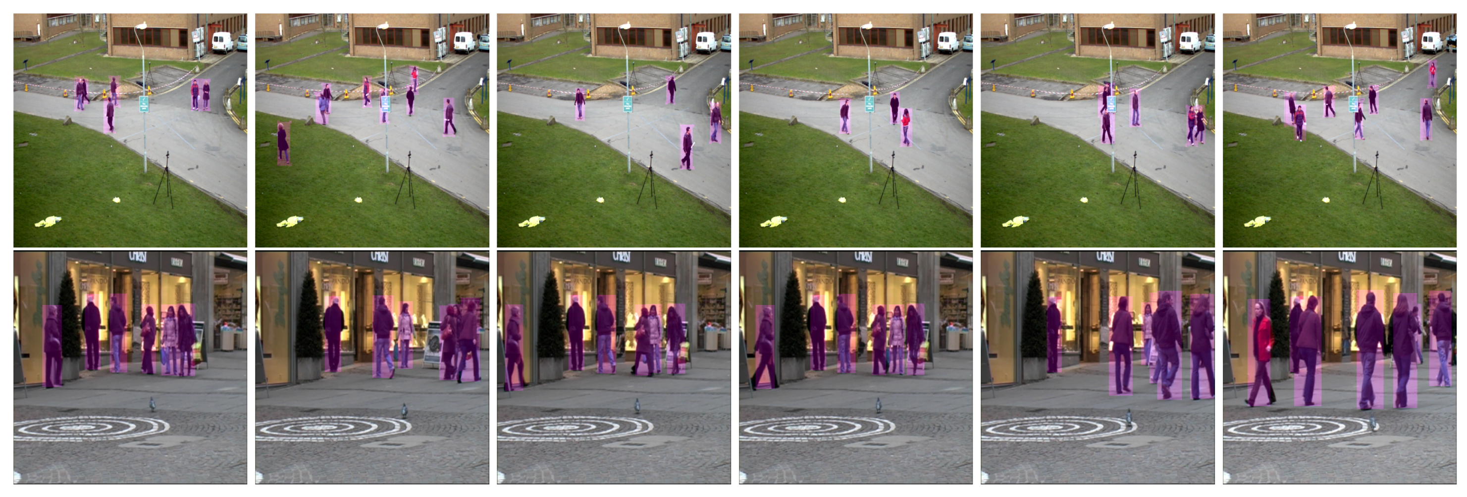
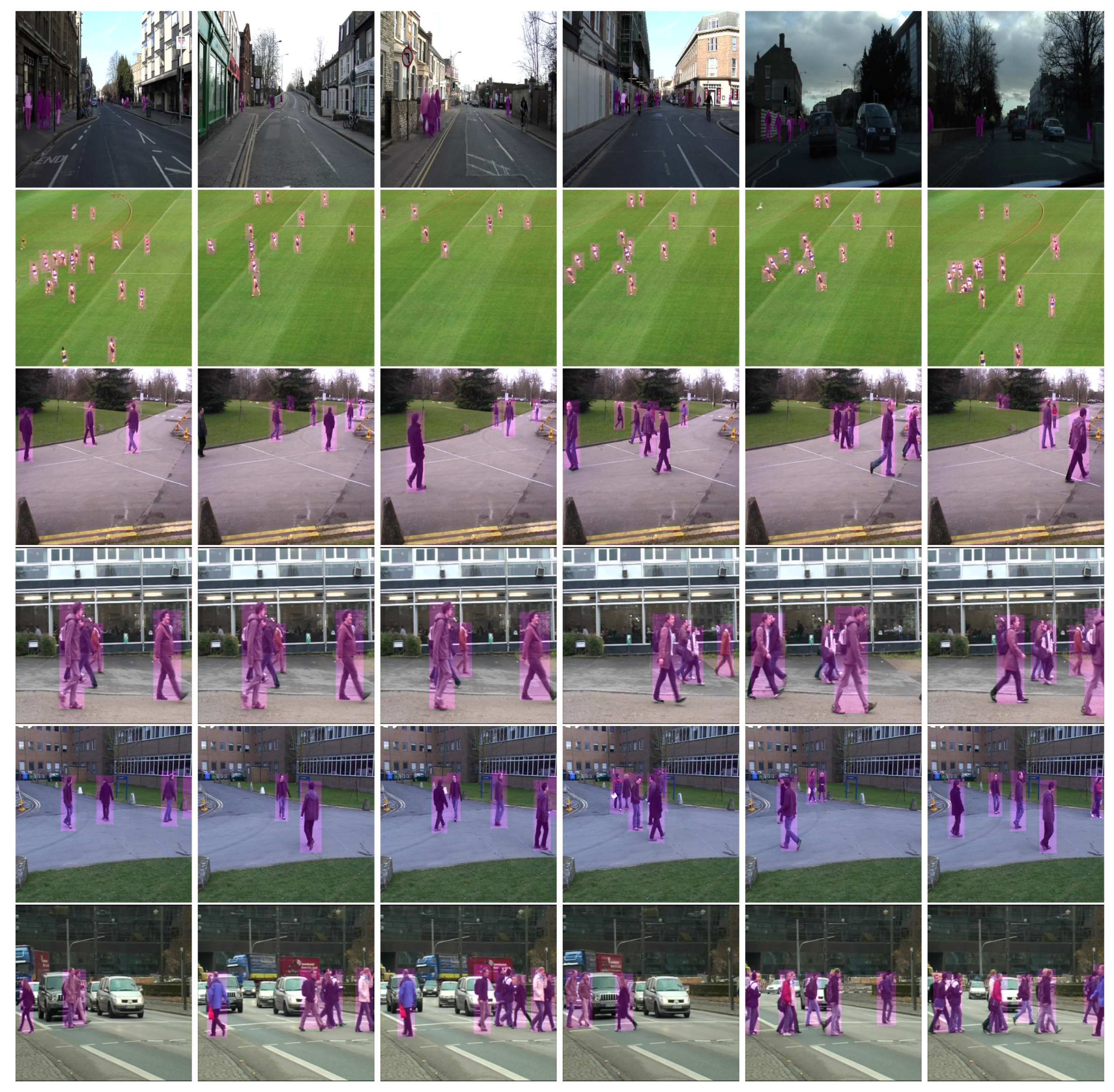
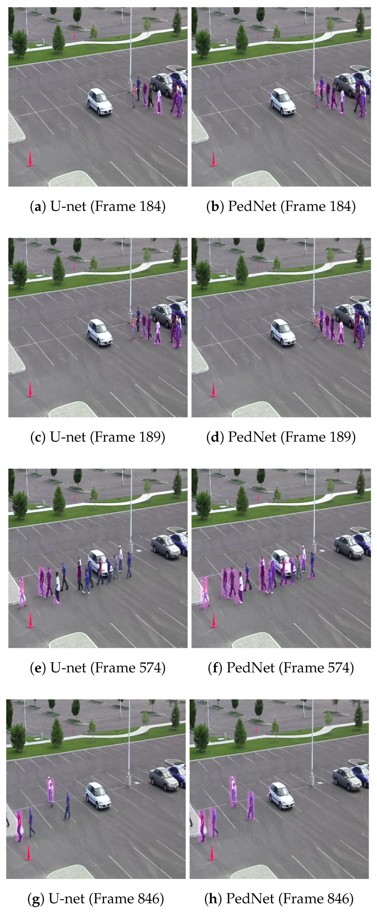
6.5. Qualitative Comparison

To show the effectiveness of our proposed PedNet, we trained U-net [5] on our own dataset. U-net has a very similar architecture to PedNet but does not use multi-frames for segmentation. We tested U-net and PedNet on the parking-lot [44,45] dataset. The parking-lot dataset was not included in the training set of either network. The Figure 7 show example frames where PedNet performs well and U-net fails to segment regions corresponds to the pedestrian.

7. Discussion and Future Work

Deep learning models have shown outstanding performance on segmentation compared to hand-crafted features based models. However, all the deep models only rely on visual learned features. Our work is first effort to incorporate the temporal information in the deep network for segmentation. After training the network, the network should be able to extract different information from the frames at t 1 , t, and t + 1 . To prove our claim, we used Grad-CAM [43] to visualize the activations of the layers. The visualization showed that the response of the network is different on each frame. Hence, the network learned to combine the optimal temporal features for spatial segmentation. Furthermore, we tested the parking-lot dataset which the network has never seen. The qualitative results show that PedNet successfully segments the regions in frames corresponding to the pedestrians. We trained the current architecture only for a single class i.e., pedestrian. However, it could be trained for any other class and potentially, for multi-classes. While evaluating the network, it was challenging to find relevant datasets. As almost all the segmentation datasets like Pascal VOC consist of single-frames. However, our model needs sequential data in order to exploit the temporal information for segmentation. The datasets that is commonly used for tracking pedestrian was a good fit to evaluate our model. Moreover, we evaluated the model on CamVid which is most commonly used for segmentation. In future, our aim is to train the network for more than one classes and also increase the temporal window i.e., rather than considering only three frames, consider a batch of frames for even more temporal rich information.

8. Conclusions

We proposed a spatio-temporal deep convolutional neural network that exploits temporal information for spatial segmentation. The backbone of our architecture consists of an encoder–decoder network for downsampling and upsampling the feature maps, receptively. For boundary delineation of the segmented mask, long-skip connections are introduced which helps to combine the low-level fine-grained features with high-level semantic information. The network is trained end-to-end from scratch. Two types of data augmentations are used which enhances the network generalization and avoid the problem of under-fitting. Different layers of the network are visualized and the maximum response of the consecutive frames are calculated through Grad-CAM. The variance in the response showed that the network is forced to learn features from the previous and future frame for spatial segmentation of the current frame. We evaluated the network on 8 datasets and achieved state-of-the-art performance. Qualitative results are also shown against single-frame segmentation approaches and the effectiveness of temporal information has been proved.

Author Contributions

M.U. is the first author of the paper. His contributions consist of methodology, data collection, implementation, testing, and writing. A.M. helped in implementation and guided the research work. F.A.C. supervised the whole research project.

Funding

This research is funded by the Norwegian ministry of education and research council of Norway through project No. KD:68123734 and IQ-MED:247689.

Conflicts of Interest

The authors declare no conflict of interest.

References

  1. Coşar, S.; Donatiello, G.; Bogorny, V.; Garate, C.; Alvares, L.O.; Brémond, F. Toward abnormal trajectory and event detection in video surveillance. IEEE Trans. Circuits Syst. Video Technol. 2017, 27, 683–695. [Google Scholar] [CrossRef]
  2. Ullah, M.; Ullah, H.; Conci, N.; De Natale, F.G. Crowd behavior identification. In Proceedings of the IEEE International Conference on Image Processing (ICIP), Phoenix, AZ, USA, 25–28 September 2016; pp. 1195–1199. [Google Scholar]
  3. Kiy, K. Segmentation and detection of contrast objects and their application in robot navigation. Pattern Recognit. Image Anal. 2015, 25, 338–346. [Google Scholar] [CrossRef]
  4. Szegedy, C.; Liu, W.; Jia, Y.; Sermanet, P.; Reed, S.; Anguelov, D.; Erhan, D.; Vanhoucke, V.; Rabinovich, A. Going deeper with convolutions. In Proceedings of the IEEE Conference on Computer Vision and Pattern Recognition (CVPR), Boston, MA, USA, 7–12 June 2015; pp. 1–9. [Google Scholar]
  5. Ronneberger, O.; Fischer, P.; Brox, T. U-net: Convolutional networks for biomedical image segmentation. In Proceedings of the International Conference on Medical Image Computing and Computer-Assisted Intervention (MICCAI), Munich, Germany, 5–9 October 2015; Springer: Berlin, Germany, 2015; pp. 234–241. [Google Scholar]
  6. Gowsikhaa, D.; Abirami, S.; Baskaran, R. Automated human behavior analysis from surveillance videos: A survey. Artif. Intell. Rev. 2014, 42, 747–765. [Google Scholar] [CrossRef]
  7. Farabet, C.; Couprie, C.; Najman, L.; LeCun, Y. Learning hierarchical features for scene labeling. IEEE Trans. Pattern Anal. Mach. Intell. 2013, 35, 1915–1929. [Google Scholar] [CrossRef] [PubMed] [Green Version]
  8. Hariharan, B.; Arbeláez, P.; Girshick, R.; Malik, J. Simultaneous detection and segmentation. In Proceedings of the European Conference on Computer Vision (ECCV), Zurich, Switzerland, 6–12 September 2014; Springer: Berlin, Germany, 2014; pp. 297–312. [Google Scholar]
  9. Gupta, S.; Girshick, R.; Arbeláez, P.; Malik, J. Learning rich features from RGB-D images for object detection and segmentation. In Proceedings of the European Conference on Computer Vision (ECCV), Zurich, Switzerland, 6–12 September 2014; Springer: Berlin, Germany, 2014; pp. 345–360. [Google Scholar]
  10. Sturgess, P.; Alahari, K.; Ladicky, L.; Torr, P.H. Combining appearance and structure from motion features for road scene understanding. In Proceedings of the British Machine Vision Conference (BMVC), London, UK, 7–10 September 2009; Springer: Berlin, Germany, 2009. [Google Scholar]
  11. Ladickỳ, L.; Sturgess, P.; Alahari, K.; Russell, C.; Torr, P.H. What, where and how many? combining object detectors and crfs. In Proceedings of the European Conference on Computer Vision (ECCV), Heraklion, Crete, Greece, 5–11 September 2010; Springer: Berlin, Germany, 2010; pp. 424–437. [Google Scholar]
  12. Shotton, J.; Johnson, M.; Cipolla, R. Semantic texton forests for image categorization and segmentation. In Proceedings of the IEEE Conference on Computer Vision and Pattern Recognition (CVPR), Anchorage, AK, USA, 23–28 June 2008; pp. 1–8. [Google Scholar]
  13. Brostow, G.J.; Shotton, J.; Fauqueur, J.; Cipolla, R. Segmentation and recognition using structure from motion point clouds. In Proceedings of the European Conference on Computer Vision, Marseille, France, 12–18 October 2008; Springer: Berlin, Germany, 2008; pp. 44–57. [Google Scholar]
  14. Dalal, N.; Triggs, B. Histograms of oriented gradients for human detection. In Proceedings of the IEEE Conference on Computer Vision and Pattern Recognition (CVPR), San Diego, CA, USA, 20–25 June 2005; Volume 1, pp. 886–893. [Google Scholar]
  15. Yang, Y.; Li, Z.; Zhang, L.; Murphy, C.; Ver Hoeve, J.; Jiang, H. Local label descriptor for example based semantic image labeling. In Proceedings of the European Conference on Computer Vision (ECCV), Florence, Italy, 7–13 October 2012; Springer: Berlin, Germany, 2012; pp. 361–375. [Google Scholar]
  16. Elad, M. Sparse and redundant representation modeling—What next? IEEE Signal Process. Lett. 2012, 19, 922–928. [Google Scholar] [CrossRef]
  17. Kontschieder, P.; Bulo, S.R.; Bischof, H.; Pelillo, M. Structured class-labels in random forests for semantic image labelling. In Proceedings of the IEEE International Conference on Computer Vision (ICCV), Barcelona, Spain, 6–13 November 2011; pp. 2190–2197. [Google Scholar]
  18. Zhang, C.; Wang, L.; Yang, R. Semantic segmentation of urban scenes using dense depth maps. In Proceedings of the European Conference on Computer Vision (ECCV), Heraklion, Crete, Greece, 5–11 September 2010; Springer: Berlin, Germany, 2010; pp. 708–721. [Google Scholar]
  19. Ren, X.; Bo, L.; Fox, D. Rgb-(d) scene labeling: Features and algorithms. In Proceedings of the IEEE Conference on Computer Vision and Pattern Recognition (CVPR), Providence, RI, USA, 16–21 June 2012; pp. 2759–2766. [Google Scholar]
  20. Bo, L.; Ren, X.; Fox, D. Depth kernel descriptors for object recognition. In Proceedings of the IEEE International Conference on Intelligent Robots and Systems (IROS), San Francisco, CA, USA, 25–30 September 2011; pp. 821–826. [Google Scholar]
  21. Krizhevsky, A.; Sutskever, I.; Hinton, G.E. Imagenet classification with deep convolutional neural networks. In Proceedings of the Advances in Neural Information Processing Systems (NIPS), Lake Tahoe, NV, USA, 3–6 December 2012; pp. 1097–1105. [Google Scholar]
  22. Zeiler, M.D.; Fergus, R. Visualizing and understanding convolutional networks. In Proceedings of the European Conference on Computer Vision (ECCV), Zurich, Switzerland, 6–12 September 2014; pp. 818–833. [Google Scholar]
  23. He, K.; Zhang, X.; Ren, S.; Sun, J. Deep residual learning for image recognition. arXiv, 2015; arXiv:1512.03385. [Google Scholar]
  24. Simonyan, K.; Zisserman, A. Very deep convolutional networks for large-scale image recognition. arXiv, 2014; arXiv:1409.1556. [Google Scholar]
  25. Badrinarayanan, V.; Kendall, A.; Cipolla, R. Segnet: A deep convolutional encoder–decoder architecture for image segmentation. IEEE Trans. Pattern Anal. Mach. Intell. 2017, 39, 2481–2495. [Google Scholar] [CrossRef] [PubMed]
  26. Chen, L.C.; Papandreou, G.; Kokkinos, I.; Murphy, K.; Yuille, A.L. Deeplab: Semantic image segmentation with deep convolutional nets, atrous convolution, and fully connected crfs. IEEE Trans. Pattern Anal. Mach. Intell. 2018, 40, 834–848. [Google Scholar] [CrossRef] [PubMed]
  27. Lin, G.; Milan, A.; Shen, C.; Reid, I. Refinenet: Multi-path refinement networks for high-resolution semantic segmentation. In Proceedings of the IEEE Conference on Computer Vision and Pattern Recognition (CVPR), Honolulu, HI, USA, 21–26 July 2017; Volume 1, p. 3. [Google Scholar]
  28. Henaff, M.; Weston, J.; Szlam, A.; Bordes, A.; LeCun, Y. Tracking the world state with recurrent entity networks. arXiv, 2016; arXiv:1612.03969. [Google Scholar]
  29. Vaswani, A.; Shazeer, N.; Parmar, N.; Uszkoreit, J.; Jones, L.; Gomez, A.N.; Kaiser, Ł.; Polosukhin, I. Attention is all you need. In Proceedings of the Advances in Neural Information Processing Systems (NIPS), Long Beach, CA, USA, 4–9 December 2017; pp. 6000–6010. [Google Scholar]
  30. Noh, H.; Hong, S.; Han, B. Learning deconvolution network for semantic segmentation. In Proceedings of the IEEE International Conference on Computer Vision, Santiago, Chile, 7–13 December 2015; pp. 1520–1528. [Google Scholar]
  31. Long, J.; Shelhamer, E.; Darrell, T. Fully convolutional networks for semantic segmentation. In Proceedings of the IEEE Conference on Computer Vision and Pattern Recognition (CVPR), Boston, MA, USA, 7–12 June 2015; pp. 3431–3440. [Google Scholar]
  32. Chen, L.C.; Papandreou, G.; Kokkinos, I.; Murphy, K.; Yuille, A.L. Semantic image segmentation with deep convolutional nets and fully connected crfs. arXiv, 2014; arXiv:1412.7062. [Google Scholar]
  33. Zanjani, F.G.; van Gerven, M. Improving Semantic Video Segmentation by Dynamic Scene Integration. In Proceedings of the NCCV 2016: The Netherlands Conference on Computer Vision, Lunteren, The Netherlands, 12–13 December 2016. [Google Scholar]
  34. Shelhamer, E.; Rakelly, K.; Hoffman, J.; Darrell, T. Clockwork convnets for video semantic segmentation. In Proceedings of the European Conference on Computer Vision (ECCV), Amsterdam, The Netherlands, 8–16 October 2016; Springer: Berlin, Germany, 2016; pp. 852–868. [Google Scholar]
  35. Luc, P.; Neverova, N.; Couprie, C.; Verbeek, J.; LeCun, Y. Predicting deeper into the future of semantic segmentation. In Proceedings of the IEEE International Conference on Computer Vision (ICCV), Venice, Italy, 22–29 October 2017; Volume 1. [Google Scholar]
  36. Ferryman, J.; Shahrokni, A. Pets2009: Dataset and challenge. In Proceedings of the Twelfth IEEE International Workshop on Performance Evaluation of Tracking and Surveillance (PETS-Winter), Snowbird, UT, USA, 7–9 December 2009; pp. 1–6. [Google Scholar]
  37. Andriluka, M.; Roth, S.; Schiele, B. Monocular 3D pose estimation and tracking by detection. In Proceedings of the IEEE Conference on Computer Vision and Pattern Recognition, San Francisco, CA, USA, 13–18 June 2010; pp. 623–630. [Google Scholar]
  38. Andriluka, M.; Roth, S.; Schiele, B. People-tracking-by-detection and people-detection-by-tracking. In Proceedings of the IEEE Conference on Computer Vision and Pattern Recognition, Anchorage, AK, USA, 23–28 June 2008; pp. 1–8. [Google Scholar]
  39. Brostow, G.J.; Fauqueur, J.; Cipolla, R. Semantic object classes in video: A high-definition ground truth database. Pattern Recognit. Lett. 2009, 30, 88–97. [Google Scholar] [CrossRef]
  40. Milan, A.; Gade, R.; Dike, A.; Moeslund, T.B.; Ian, R. Improving global multi-target tracking with local updates. In Proceedings of the European Conference on Computer Vision, Zurich, Switzerland, 6–12 September 2014; Springer: Cham, Switzerland, 2014; pp. 174–190. [Google Scholar]
  41. Hinton, G.; Srivastava, N.; Swersky, K. Rmsprop: Divide the gradient by a running average of its recent magnitude. Neural Netw. Mach. Learn. 2012, 4, 26–31. [Google Scholar]
  42. Glorot, X.; Bengio, Y. Understanding the difficulty of training deep feedforward neural networks. In Proceedings of the Thirteenth International Conference on Artificial Intelligence and Statistics, Sardinia, Italy, 13–15 May 2010; pp. 249–256. [Google Scholar]
  43. Selvaraju, R.R.; Das, A.; Vedantam, R.; Cogswell, M.; Parikh, D.; Batra, D. Grad-cam: Why did you say that? visual explanations from deep networks via gradient-based localization. CoRR 2016, 7. [Google Scholar] [CrossRef]
  44. Shu, G.; Dehghan, A.; Oreifej, O.; Hand, E.; Shah, M. Part-based Multiple-Person Tracking with Partial Occlusion Handling. In Proceedings of the IEEE Conference on Computer Vision and Pattern Recognition, Providence, RI, USA, 16–21 June 2012; pp. 1815–1821. [Google Scholar]
  45. Dehghan, A.; Assari, S.M.; Shah, M. GMMCP-Tracker: Globally Optimal Generalized Maximum Multi Clique Problem for Multiple Object Tracking. In Proceedings of the IEEE Conference on Computer Vision and Pattern Recognition, Boston, MA, USA, 7–12 June 2015; pp. 4091–4099. [Google Scholar]
Figure 1. PedNet: proposed architecture. The input to the network is set of three frames at time instant t 1 , t, and t + 1. The network learned visual and temporal features and exploit it for spatial segmentation. The output is a binary mask which shows the region belonging to a pedestrian in the middle frame.
Jimaging 04 00107 g001
Figure 2. Qualitative results of our PedNet on 8 Challenging datasets. The row 1, 5, and 7 shows Pets2009 [36] dataset that is the commonly used for tracking. Second, sixth and the eighth row corresponds to TUD [37,38] dataset which is also used for evaluating tracking algorithms. The third row shows CamVid [39] dataset which is used for segmentation. The fourth row shows AFL [40] dataset which is used for tracking sports player.
Jimaging 04 00107 g002aJimaging 04 00107 g002b
Figure 3. While training the network, the samples are randomly selected from the training set. With 50% probability, the original training sample is used for training. With the other 50% probability, it can go through two types of augmentation i.e., either scaling of light intensity variation. Scaling is introduced by cropping a random region in the original frame. While light intensity variation, first Gaussian blur is applied and then gamma correction is used.
Jimaging 04 00107 g003
Figure 4. The first column shows the original frame. The 2nd column corresponds to the scaled version of the frame. The third column shows different lighting condition that is introduced through the Gaussian noise and gamma correction. The fourth column corresponds to the binary mask for training the network.
Jimaging 04 00107 g004
Figure 5. The first column shows the original frames of Pets2009 S2L1 View 1 [36] dataset. The 2nd column corresponds to the activation of Conv2d_2 for frame at t 1 , Conv2d_4 for frame at t, and Conv2d_6 for frame at t. The third and fourth column shows the original frame of Pets2009 S2L1 View 7 [36] dataset and their corresponding activation. The layers Conv2d_2, Conv2d_4, and Conv2d_6 learned different features during training, therefore, their response is different.
Jimaging 04 00107 g005
Figure 6. The activation of layer Conv2d_27 achieved through Grad-CAM [43]. It is the 2nd last layer in the decoder network and shows the maximum response of the network on the middle frame given the three input frames.
Jimaging 04 00107 g006
Figure 7. U-net [5] and PedNet are trained on the training datasets. The first column shows the result of U-net while the second column shows the result of PedNet. Even though PedNet has never seen Parking-lot [44,45] dataset, it gives better segmentation results.
Jimaging 04 00107 g007
Table 1. A detailed configuration of PedNet. “En_Conv” and “Dec_Conv” corresponds to the convolution in the encoder and decoder network. Batch normalization and ReLu are omitted from the table for clarity but each convolution is followed by these two layers.
LayerFilterParamOutput
Input-1--512 × 512 × 3
Input-2--512 × 512 × 3
Input-3--512 × 512 × 3
En_Conv2D-13 × 3224512 × 512 × 8
En_Conv2D-33 × 3896512 × 512 × 32
En_Conv2D-53 × 3224512 × 512 × 8
En_Conv2D-23 × 3584512 × 512 × 8
En_Conv2D-43 × 39248512 × 512 × 32
En_Conv2D-63 × 3584512 × 512 × 8
Concat_1--512 × 512 × 48
En_Conv2D-73 × 313,856512 × 512 × 32
En_Pool2D-12 × 2-256 × 256 × 32
En_Conv2D-83 × 318,496256 × 256 × 64
En_Conv2D-93 × 336,928256 × 256 × 64
En_Pool2D-22 × 2-128 × 128 × 64
En_Conv2D-103 × 373,856128 × 128 × 128
En_Conv2D-113 × 3147,584128 × 128 × 128
En_Pool2D-32 × 2-64 × 64 × 128
En_Conv2D-123 × 3295,16864 × 64 × 256
En_Conv2D-133 × 3590,08064 × 64 × 256
En_Pool2D-42 × 2-32 × 32 × 256
En_Conv2D-143 × 31,180,16032 × 32 × 512
En_Conv2D-153 × 32,359,80832 × 32 × 512
En_Pool2D-52 × 2-16 × 16 × 512
En_Conv2D-163 × 34,719,61616 × 16 × 1024
En_Conv2D-173 × 39,438,20816 × 16 × 1024
Dec_UpSample2D-12 × 2-32 × 32 × 1024
Concat-2--32 × 32 × 1536
Dec_Conv2D-183 × 37,078,40032 × 32 × 512
Dec_Conv2D-193 × 32,359,80832 × 32 × 512
Dec_UpSample2D-22 × 2-64 × 64 × 512
Dec_Conv2D-183 × 37,078,40032 × 32 × 512
Dec_Conv2D-193 × 32,359,80832 × 32 × 512
Dec_UpSample2D-22 × 2-64 × 64 × 512
Concat-3--64 × 64 × 768
Dec_Conv2D-203 × 31,769,72864 × 64 × 256
Dec_Conv2D-213 × 3590,08064 × 64 × 256
Dec_UpSample2D-32 × 2-128 × 128 × 256
Concat-4--128 × 128 × 384
Dec_Conv2D-223 × 344,2496128 × 128 × 128
Dec_Conv2D-233 × 3147,584128 × 128 × 128
Dec_UpSample2D-42 × 2-256 × 256 × 128
Concat-5--256 × 256 × 192
Dec_Conv2D-243 × 3110,656256 × 256 × 64
Dec_Conv2D-253 × 336,928256 × 256 × 64
Dec_UpSample2D-52 × 2-512 × 512 × 64
Concat-6--512 × 512 × 96
Dec_Conv2D-263 × 313,840512 × 512 × 16
Dec_Conv2D-273 × 32320512 × 512 × 16
Dec_Conv2D-283 × 317512 × 512 × 1
Table 2. Quantitative results of our PedNet on 8 different datasets.
DatasetsRecallPrecisionF 1 F 2 mIoUAccuracy
CamVid0.8770.9450.9100.8900.7640.988
Pets2009 (View 1 )0.8830.9530.9170.8960.7550.989
TUD-crossing0.8800.9550.9160.8940.7410.989
AFL-football0.8800.9550.9160.8940.7460.987
Pets2009 (view 5 )0.8770.9430.9090.8890.7240.988
Pets2009 (view 7 )0.8780.9490.9120.8910.7670.989
TUD-Stadmitt0.8800.9550.9160.8940.7410.988
TUD-Campus0.8860.9440.9140.8970.6920.989
Table 3. Quantitative results of our PedNet against state-of-the-art methods on CamVid dataset. The results of [10,11,17] are based on hand-crafted features. The results of [25,30,31,32] are based on deep model. It is apparent that the deep model outperforms the classical approaches and our PedNet outperformed the deep models by a good margin.
MethodsmIoUAccuracy
SegNet [25]0.5000.888
Ladicky et al. [11]-0457
Chen et al. [32]0.5010.859
Long et al. [31]0.5600.832
Noh et al. [30]0.3960.852
Kontschider et al. [17]-0.430
Sturgess et al. [10]-0.536
Ours PedNet0.7640.988

