Viewing Experience Model of First-Person Videos


School of Electrical and Computer Engineering, Purdue University, West Lafayette, IN 47907, USA
*
Author to whom correspondence should be addressed.
J. Imaging 2018, 4(9), 106; https://doi.org/10.3390/jimaging4090106
Submission received: 28 May 2018
/
Revised: 11 August 2018
/
Accepted: 27 August 2018
/
Published: 31 August 2018
(This article belongs to the Special Issue Image Quality)
Abstract
:First-Person Videos (FPVs) are recorded using wearable cameras to share the recorder’s First-Person Experience (FPE). Ideally, the FPE is conveyed by the viewing experience of the FPV. However, raw FPVs are usually too shaky to watch, which ruins the viewing experience. To solve this problem, we improve the viewing experience of FPVs by modeling it as two parts: video stability and First-Person Motion Information (FPMI). Existing video stabilization techniques can improve the video stability but damage the FPMI. We propose a Viewing Experience (VE) score, which measures both the stability and the FPMI of a FPV by exploring the mechanism of human perception. This enables us to further develop a system that can stabilize FPVs while preserving their FPMI so that the viewing experience of FPVs is improved. Objective tests show that our measurement is robust under different kinds of noise, and our system has competitive performance relative to current stabilization techniques. Subjective tests show that (1) both our stability and FPMI measurements can correctly compare the corresponding attributes of an FPV across different versions of the same content, and (2) our video processing system can effectively improve the viewing experience of FPVs.
1. Introduction
With the development of wearable cameras, people are starting to create First-Person Videos (FPVs) to record their life. Some producers even make First-Person films. From simple life-logs to playing sports, the content of FPVs varies dramatically. Recorders usually share a common primary goal: sharing their First-Person Experience (FPE) with others. However, the fact is that the viewing experience of FPVs is quite different from the recorder’s FPE. In this paper, we start by discussing the reason behind this fact and create a reliable solution that enables us to improve the viewing experience of FPVs based on a viewing experience model. As a result, recorders’ FPEs can be effectively conveyed to viewers.
Our problem can be addressed by comparing the attributes of both the FPE and the viewing experience of FPVs and accordingly adjusting the attributes of the latter. We begin by modeling the attributes of the FPE. Recorders are eager to share two aspects of the FPE. First, recorders would like to share the objective information they perceive. For example, if a recorder captures an FPV when he/she is running in a park, he/she may want to share the trees or flowers with viewers. Second, recorders would like to share the feeling of interacting in the First-Person perspective, i.e., the subjective information they perceived from the objective world. Using the same example, the recorder may want to share his/her reaction and interest to a dog that barks behind him/her as he/she turns around to look at the dog.
The viewing experience of FPVs has different attributes, which includes video stability and First-Person Motion Information (FPMI). The FPMI corresponds to the FPE and includes both the objective and subjective information conveyed by camera motion. Video instability does not have a corresponding concept in FPE, because it is not experienced in real life. Usually, viewers feel that FPVs are too shaky to watch, but recorders never feel dizzy when they record the video. They never even realize that there are stability-related issues. Later in this paper, we show that this is because the visual function we apply when we watch the FPVs is different from the visual function that we rely on when we experience real-life. As a result, to help recorders to share FPE, we propose it is important to
- (1)
- Preserve FPMI;
- (2)
- Fix the unpleasant component, that is, increase video stability.
In this work, we propose a system to improve the viewing experience of FPVs by stabilizing them while preserving their FPMI. To achieve this, we construct measurements of video stability and FPMI for FPVs based on a human perception model.
In the next section, we review several off-the-shelf approaches which are related to our problem, such as traditional video stabilization techniques. However, we show that these methods are insufficient. In Section 3, we provide an overview of our system. Following the pipeline of our system, its subparts are introduced from Section 4, Section 5, Section 6 and Section 7. Section 4 focuses on the motion estimation algorithm which is a modified visual odometer according to the difference between our task and traditional stabilization tasks. The human perception model based on eye movements is the basis of our system, and is presented in Section 5. By applying the human perception model, we propose the quality metric of the viewing experience of FPVs in Section 6. We edit camera motion using the quality metric to improve the viewing experience, which is shown in Section 7. Section 8 includes three parts of our experimental results. First, we design and use subjective tests to finalize the parameters in our human perception model. Second, objective and subjective tests are employed to test the robustness of our viewing experience measurement. Third, subjective tests show the effectiveness of our system in comparison with other methods.
This paper is based on our three conference papers [1,2,3]. In Ref. [1], we proposed the prototype of our current system without an accurate perception model. In Ref. [2], we improved the system by proposing an accurate mathematical perception model based on eye motion, and in Ref. [3], we performed subjective tests to help us explore the parameter setting in the mathematical perception model.
This current paper incorporates these settings into our complete system and provides a cohesive description of the structure and theory of the entire system. We update the experiments, which compare the performance of our system with state-of-art systems. We enhance the figures to help explain the mathematical model more clearly. In addition, we present new discussions about the relationship between motion and the video viewing experience. These results have not been included in our previous work and are valuable for many applications, such as video quality, digital video stabilization, gimbal design, and First-Person game design.
Note that we define several new concepts here. For readers’ convenience, we summarize them in Table 1.
2. Related Work
2.1. Video Stabilization
As we discussed, the viewing experience of FPVs includes two parts: video stability and FPMI. Traditional video stabilization techniques can effectively remove the shakiness within FPVs, but they either have limited performance on FPVs or damage the FPMI with high probability. However, these traditional methods still provide some valuable concepts.
Traditional video stabilization techniques include hardware-based methods and software-based methods. Examples of hardware-based video stabilization techniques include the built-in functions of cameras such as GoPro Hero 5/6 and other hand-held stabilizers. The problem with these solutions is that they have limited performance. The built-in function in GoPro Hero 5/6 can only remove small amounts of shakiness since the camera records in real-time and must avoid obvious stitching errors when applying the stabilization function. Hand-held stabilizers require users to hold the device, which limits the users’ activities to riding or driving. Although wearable gimbals are available, their current designs are still large and heavy for users who want to record for long-period activities.
To stabilize a video using a software-based method, three steps are performed: motion estimation, motion smoothing, and frame/video reforming. The problem of these methods is that their motion smoothing step damages the FPMI of the FPV, since the purpose of these methods is to stabilize videos as much as possible. They are still valuable if they can be guided by an accurate video stability estimator so that users know how much stabilization can be used without damaging the FPMI.
Based on the motion type they are designed for, the video stabilization techniques are classified into 2D [4,5,6,7] and 3D solutions [8,9,10,11]. In the 2D solutions, the motion on the image plane is estimated using either local features or pixel intensity information. Then, the frame transformation is calculated based on the smoothed 2D motion. In contrast, 3D solutions estimate the camera motion in the 3D world. The estimation approaches mainly rely on the methods of either structure-from-motion (SfM) [12] or visual-based simultaneous localization and mapping (vSLAM) [13]. The advantage of 3D solutions is that they generate a full understanding of the physical camera motions. However, they are usually slower and more fragile than 2D methods, since their motion estimation step is sensitive to the accuracy of feature matching [4,6,9]. The drawback of 2D methods is that they do not have an understanding of the 3D world, so users cannot obtain a real ideal camera path like the ones that 3D methods can provide. As a result, some advanced processes, such as intentional motion preservation, cannot be performed. Also, in most cases, these algorithms would produce severe distortions when the recorded scene cannot be modeled as planar.
To precisely edit the camera motion to improve video stability and preserve FPMI, we adopted a 3D video stabilization pipeline in this paper.
2.2. Stability Measurements
As we discussed, to correctly operate the video stabilization algorithms, an accurate video stability estimator is needed. Some stability measurements have been proposed along with video stabilization techniques. In fact, many video stabilization techniques are not based on measurements [6,9,14,15,16]. Since they do not rely on any measurement, their smoothing parameters are not adaptive, and thus, the stabilization process is not controllable. However, other video stabilization techniques [4,5,7,8,17] implicitly generate stability measurements as by-products. Their smoothing step is based on optimization processes that minimize the sum of the squared values of the second derivatives of the motion curves. Some also use other similar objective functions. For example, in Ref. [5], the mean square value of the third derivative was also used, and the difference between the simplified affine motion parameters between adjacent frames was used in Ref. [17].
Inter-frame transformation fidelity (ITF) was proposed in Ref. [18] for surveillance applications and has been used by many authors [19,20,21,22] to compare the performances of different stabilization methods. First, the peak signal-to-noise ratio (PSNR) between adjacent frames are computed. The mean PSNR of all adjacent pairs is the ITF which can be easily and quickly computed. The motion-based mean squared error (MV-MSE) [23] is another valuable stability estimator which is a full-reference stability estimator. The MV-MSE is also easy to compute. First, the intentional camera motion needs to be computed. For example, in Ref. [23], the original motion was transformed into the frequency domain and low-pass filtered to generate the intentional motion. Then, the quality score was the MSE between the intentional motion and the original one. The mean squared error was decomposed in Ref. [24] into jitter and divergence in an effort to further interpret the MV-MSE.
The drawback of these stability measurements is that they cannot precisely predict the subjective stability. The measurements used by video stabilization techniques assume that fast motion is the reason for instability. However, the numerical relationship between motion speed and instability is unknown. Also, it is well-known that PSNR does not have high correlation with subjective quality scores [25,26]. In addition, MV-MSE only measures the relative stability between the original motion and the intentional motion. Moreover, the intentional motion is just estimated, because the actual intended motion is unknown. In this paper, we show that the subjective stability of intentional motion strictly depends on its amplitude and frequency characteristics which means intentional motion is seldom completely stable. As a result, MV-MSE cannot accurately measure the subjective stability of videos.
In this work, we propose a video stability measurement that can help us to predict the subjective video stability and guide us to appropriately stabilize FPVs.
2.3. FPV Enhancement Techniques
There is also some prior work that enhances FPVs [8,27,28,29]. Two factors make them different from the traditional video stabilization techniques. First, they focus on processing FPVs and share the same target that we have: to create watchable FPVs. Second, these works may solve the shakiness problem in different ways [27,28,29] or introduce additional processes to the stabilized FPVs [8].
Instead of stabilizing frames by smoothing the camera motion, Refs. [27,28,29] tried to find and eliminate the frames which cause the shakiness. After the processing, only the semantic segments, for example the segments that contain human faces, are preserved and assembled to construct the resulting video. The resulting video has reduced content and is a fast-forwarded version of the original video. However, we believe semantic meaning is not only available from selected frames, but also that there is semantic meaning in the First-Person Motions themselves. Their strategy ignores and discards this meaning, just like traditional video stabilization techniques.
Ref. [8] was the earliest work that focused on stabilizing FPVs. It used the 3D method in traditional video stabilization techniques to stabilize FPVs. However, the authors believe that FPVs are usually long which makes them boring to watch. As a result, the authors further processed the stabilized FPVs to be hyper-lapse videos which are FPVs accelerated through time. This idea is similar to the ones discussed above [27,28,29]. However, the accelerating rate of hyperlapse videos is controllable and the entire process does not require any content understanding techniques.
Note that Ref. [8] followed the idea proposed in Ref. [9]. They believe that the shaky video needs to be stabilized in a cinematographic manner, which means the camera motion should be highly smoothed. However, this is in contrast to our assumption. As we discussed, blindly smoothing camera motion damages the FPMI of the FPV. As a result, to evaluate our assumption, we compare our results with their results in the experiment section.
3. System Overview
We adopted the pipeline of traditional video stabilization techniques shown in Figure 1. However, three main differences help our system outperform traditional algorithms on FPVs. First, we replaced the motion smoothing step with a more general motion editing step, since this is where traditional methods damage the FPMI. Within the motion editing step, we employed two procedures: measuring and improving. The failure of traditional video stabilization techniques tells us that stabilization needs to be carefully performed for FPVs. We need to precisely measure the video stability to decide how much stabilization we should apply to shaky FPVs, to avoid the same drawbacks of traditional video stabilization techniques.
Second, this motion editing step is based on a human perception model of First-Person Motion conveyed by FPVs, which has never been explicitly considered in traditional solutions. It models the eye movements of viewers as a random process. Based on this model, we propose our viewing experience measurement which estimates the fraction of the FPV that the viewer can watch comfortably. Using our measurement, we can design a new camera path that provides a more stable view while preserving the FPMI, i.e., we can improve the viewing experience. The model of human perception ensures our viewing experience improvement results are consistent with human preference.
Third, our system only edits angular motions. Based on our hypothesis, translational motion conveys the FPMI, so it should be preserved. As a result, the traditional 3D motion estimation algorithm is simplified to only extract the angular motions. This also allows us to avoid the challenge of monocular visual odometers, where computing the scale requires the local features to be observed successively in several frames. When we only compute rotations, this constraint does not apply because rotations are independent of scale.
4. Three-Dimensional Motion Estimation
Three-dimensional motion estimation, or so-called camera pose estimation, is a well-studied problem in both the computer vision and the robotics communities where it is defined as Structure-from-Motion (SfM) or visual Simultaneous Localization And Mapping (vSLAM). “Motion” or “camera pose” usually refers to both the translation and rotation of the camera. Traditional 3D video stabilization techniques apply these approaches and remove both the angular motion and the translation of the camera.
However, we do not remove, and thus do not need, to estimate the camera translations. As stated above, the translations include significant FPMI. The amplitude and frequency of translations can reflect the speed and type of movement of the recorder (e.g., running, flying, or walking). For example, if the amplitude of forward translation is high, and the amplitude and frequency of the translation in the vertical direction are also relatively high, then we may infer that the recorder is running. By applying traditional stabilization techniques, we may lose this important information, since the video would look like it was recorded using a moving tripod if the vertical translation was smoothed or removed.
Also, translations are preferred in FPVs. Their importance is evident from First-Person Video gaming, since watching an FPV is similar to playing a First-Person Video game. In First-Person Video games, the translations in the vertical and horizontal directions are called “head bobbing”. Recent First-Person Video games simulate head bobbing to make the games more realistic. For this topic, Ref. [30] provided a study and showed that most players prefer games that have head bobbing.
Since the translation is not estimated, the rotation between each two frames can be estimated independently during a first pass which is called the initialization. After that, we the pose graph is built and a graph-based optimization algorithm is applied to reduce the error introduced during the initialization step. The initialization step is operated based on SURF (Speeded Up Robust Features) [31] with RANSAC (random sample consensus) [32]. For each two frames, it is first assumed they share a large enough baseline that a triangulation can be performed successfully using epipolar geometry. When there are not enough inliers after the RANSAC, we believe the triangulation fails, and the camera motion between these two frames is a pure rotation. In this situation, the fundamental matrix degenerates to a homography.
Suppose the estimated camera pose of the ith frame is ,
where the estimated rotation from frame to frame i. Using the graph optimization tools provided by Ref. [33], we refined the estimated rotations using the objective function:
refers to the special orthogonal group which is the group of all 3D rotations. It restricts all R to be valid rotations during optimization. i and j are time indices of camera poses. L constrains the distance between frame indices. The larger l is, the further apart the two frames may be. In the experiments, we found that is large enough to have a large baseline for FPVs recorded in 30 fps. Note that this approach requires the camera’s intrinsic parameters.
These matrices in the special orthogonal group are mathematical expressions of the camera poses which do not have a physical meaning to humans. To edit camera motions, we need to decompose these matrices in the same way that humans understand camera motions. After that, we can apply the human perception model to measure the viewing experience of the camera motions.
Humans understand camera motions in the sense of Euler angles. A camera motion is usually understood as a combination of pitch, yaw, and roll, which are the rotations around the x, y, and z axes. Thus, we decompose a camera pose () into three Euler angles. However, there is no unique solution for the decomposition. In order to give the results a more realistic meaning that is closer to the understanding of humans, the decomposition order is chosen so that it coincides with the importance of human motions. Considering typical human activities, yaw, which is performed to look around, is the most important motion. Pitch, which is performed to look up and down, has intermediate importance. Roll is seldom performed intentionally, so our goal is to remove it during stabilization. As a result, the camera pose of the ith frame is decomposed as
The corresponding angles are computed as
where
and is the entry of matrix R.
Note that the entire speed of our system (including the parts we introduce in the rest of the paper) is around 6 s per frame with nearly 80% of the time spent on 3D motion estimation. In this paper, we do not focus on optimizing the motion estimation algorithm, which can be achieved by incorporating the recent work in Ref. [34].
5. Human Perception Model
The viewing experience when watching FPVs is different than our real life First-Person Experience. This is because we rely on different visual functions in these two different situations. In this section, we first introduce the human visual functions used in these two situations, which are the Vestibulo-Ocular Reflex (VOR) and Smooth Pursuit Eye Movement (SPEM). Then we describe our eye movement model of SPEM which considers the closed-loop characteristics of the human visual tracking system.
5.1. Vestibulo-Ocular Reflex
When the recorder captures FPVs in real life, they never feel dizzy. This is because their body applies the Vestibulo-Ocular Reflex (VOR) to compensate for the rotations of their head. The bio-signals from the semicircular ducts located in their ears carry the information of the amplitudes of the yaw, pitch, and roll and control the extraocular muscles to perform opposite eye motions to compensate for the head motion. As a result, the images of interesting objects can be maintained at the center of the visual field, i.e., the fovea. This process can be thought as an image stabilization function of the human body. The frequency of VOR can reach up to 100 Hz [35], which ensures the stabilization can be achieved in real-time.
5.2. Smooth Pursuit Eye Movement
When watching an FPV, the viewer performs a different eye movement to accomplish the stabilization task. The perceived motion of a passive viewer does not activate the VOR, and the semicircular ducts provide no information. Consequently, to stabilize the images, viewers can only rely on visual information and must perform Smooth Pursuit Eye Movement (SPEM).
Before the viewer starts to pursue the target, a catch-up saccade needs to be performed to catch the target, which takes nearly 150 ms [36]. A catch-up saccade is triggered when SPEM lags behind or over-shoots the target. During a catch-up saccade, little visual information is processed by the human visual system which leads to the experience of instability.
This indicates that by measuring the fraction of the video length that the SPEM is operating under, we can measure the video stability which is one of the two parts of the viewing experience of FPVs. This requires us to understand and model the operating mechanism of the catch-up saccade. A reliable triggering model was proposed in Ref. [37] in which a catch-up saccade is triggered based on the eye-crossing time () that the human brain estimates. If the is between 40 ms and 180 ms, the catch-up saccade is not triggered. is defined as
where is the angular position error, and is the relative angular speed (target’s image speed on the fovea) or so-called retinal slip. Intuitively, this ratio is the time that human eyes need to catch the target.
However, this model is not sufficient for building a measurement of viewing experience of FPVs. Next, we discuss the basic geometry of watching FPVs. By considering the practical situations, we present our mathematical model of SPEM for FPVs which forms the basis of the measuring approach described in Section 6.
5.3. Mathematical Model of SPEM for FPVs
To simply the problem, we developed the models for yaw, pitch, and roll motions separately. Suppose the viewer observes a video with a viewing distance (d), and the camera is performing a yaw/pitch motion. Figure 2 illustrates this in 3D. To help readers understand the 3D geometry, Figure 3 shows the top view of Figure 2.
Figure 2 shows the geometric relationships among the target object, camera, and viewer over time. Images from the left to right illustrate when the camera yaws from angle 0 (aligns with the coordinates) to angle and to angle and captures the object on the image plane. Images for pitch motion are similar, but the camera rotates along the x axis. For FPVs, the translation of the recorder within a short period is relatively small with respect to the depth of most objects. As a result, we assume the relative position of the target with respect to the camera center is fixed.
Suppose the target position with respect to the camera center is at frame k while the camera focal length is f. The viewing distance of the viewer is d and the estimated camera position is . So, the observation angle of the target for the viewer at frame k is
At frame , the observation angle under the coordinates of frame k changes to
The geometry of roll motion is different from yaw and pitch, as shown in Figure 4. Suppose the object is on the plane in the kth frame. Then, the position at frame is
Assume that the frame rate is 30, and the viewer performs a SPEM from frame k to frame (). Then, the and in Equation (8) at frame () can be calculated with
However, we found that it is inaccurate to directly apply the conditions given in Equation (8) for two main reasons. First, the model in Ref. [37] ignores the predictive ability of SPEM. Second, the sensitivity of the human visual system needs to be taken into consideration in practice. We improve the model given in Equation (8) by considering each of these two reasons, respectively, with the following two new conditions:
where k is the frame index, is the minimum angular resolution of human eyes, and b is the bias of position error estimation. If either one of these two conditions is satisfied, the catch-up saccade is not triggered. In the next two paragraphs, we explain each of these two conditions.
The first condition, Equation (15), addresses the fact that Equation (8) treats the SPEM as an open-loop system. In the experiments in Ref. [37], the position errors are generated by changing the target position abruptly. This weakens the predictive ability of SPEM which is a key closed-loop characteristic of SPEM [38]. In addition, Ref. [37] used laser spots or circles as the tracking target to test the SPEM properties of human eyes. This will also underestimate the predictive ability of SPEM, because, according to Ref. [39,40], the target shape can provide additional information for visual tracking. Refs. [38,41,42] also concluded that the predictive ability can be generated by scene understanding or the experiences of motion patterns. None of these factors were taken into account in Ref. [37]. A direct illustration of the failure of their model is that, without the additional information, the target may precede the gaze in both position and velocity which would create a negative value of .
In contrast, our modified constraint (15) treats the SPEM as a closed-loop system. We recognize that the viewer can utilize the additional information (i.e., target shape, scene content) to track targets. The eye movement can be accelerated before the next frame is shown which makes the retinal slip change and makes the positive and fall into the desired region. This is the reason that we introduced the absolute values in Equation (15). However, there is no widely recognized mathematical model to adjust for retinal slip [38], although most studies agree that the procedure relates to a feedback control that has constant parameters based on visual content, scene understanding, or the experiences of motion patterns [38,39,40,41,42]. As a result, to describe the characteristic of the feedback control and make our model compatible, we include an unknown bias parameter b. Later in Section 8, we design a subjective test based on real scenes to help us learn about the bias parameter. The learned parameter makes our model accurately describe the SPEM in practical situations.
The second condition, Equation (16), models a limitation of our visual system. A position error, , less than the minimum angular resolution (MAR) cannot be perceived by human eyes. In addition, the human visual system introduces an estimation error when estimating the position error. This is another reason why introducing the bias b is helpful.
Equations (15) and (16) are conditions on , the angular position of the target at frame k. Solving them for each frame and for each type of motion (yaw, pitch, or roll) gives us an interval of . Any object in the current frame that has an angular position within this interval can be tracked without having a catch-up saccade between the next two frames if the SPEM has already been performed. We defined this interval as for future convenience. contains all the information we need to compute the viewing experience of FPVs.
6. Viewing Experience Measurement
We decomposed the camera motion of a FPV into yaw, pitch, and roll sub-motions. We combined the viewing experience measures of all sub-motions into an overall viewing experience measure of the FPV. In this section, we propose two viewing experience measurements for sub-motions, which are both based on the interval of SPEM-possible object positions (). The first measurement is called the Viewing Experience (VE) score which is based on a probabilistic model. It measures the fraction of frames in a video that can be tracked using SPEM. The second measurement is called the Structure Viewing Experience (SVE) score which is a faster algorithm inspired by the VE score but without the same physical meaning. The approach of combining scores of sub-motions is presented after discussing the VE and SVE scores.
6.1. Viewing Experience Score
The VE score indicates the fraction of frames can be tracked using SPEM given the current camera motion of yaw, pitch or roll. In Section 7, we show how it can be applied to different components of First-Person Motion to obtain either the stability or FPMI of a FPV. Here, however, we show how a single VE score is computed for a given motion.
Suppose we want to compute the VE of a yaw or a pitch motion. is the interval that indicates the object positions for which SPEM is possible. To unify the coordinate of all frames, we add the camera position () to . Recall that was computed in Section 4 for frame k:
In Figure 5, the upper and lower boundaries show an example of . Unlike , includes not only the positions for which SPEM is possible of each single frame but also incorporates the spatial relationship between the intervals across the duration of the video.
Consider the example in Figure 5. The eye movements of the viewer are modeled as a random process. Suppose the viewer randomly chooses a target to track within the field of view (FOV) from the first frame. The trajectory of this target in Figure 5 is a straight, horizontal line, since it remains at the same object position within a short period with respect to the camera orientation in the first frame. When this line intersects the boundaries (), the viewer can no longer track this target. In this situation, one of two things happens. To keep tracking the same target, the viewer can perform a catch-up saccade. Otherwise, a saccade eye movement is performed to randomly retarget a new object within the FOV. Either of these two procedures takes time, nearly 6 frames [36].
The procedure of targeting and maintaining smooth pursuit is defined here as a trail of tracking. A possible path of watching a video consists of several trails of tracking. By calculating the length of each possible path and their probability, we can find the expected value of the fraction of frames for which the viewer performs SPEM. Intuitively, a wider, more open pathway between the upper and lower bounds (shown in Figure 5), will produce a higher expected value, i.e., a higher VE score. This indicates that there are likely to be fewer catch-up saccades while watching the video.
First, we compute the probability of a single tracking trail. is defined as the event:
Define to be the event:
Then, we have the probability that a target is tracked from frame k and lost at frame :
where
Note that here we assume the viewer will choose any target in the frame within the FOV with equal chance.
The probability of a possible path is the cumulative product of the probability of all its tracking trails. Suppose for an -frame video, a possible path has n trails of tracking. Then, the probability of is
where encodes the start frame index of each trail of tracking in .
The length of this possible path is
The reason that the current tracking procedure lasts 6 frames before the next tracking procedure (i.e., from frame to frame ) is that there will be a 6-frame-length catch-up saccade period before the next tracking starts at frame .
Our VE score of a video from frame k to frame () can be computed as
which depends on , the camera motion.
The reason we calculate a VE score for only a few frames (from k to frame ()) instead of the whole video is that objects may only be visible for a short period. To compute Equation (22), we first identify all the possible paths for a length () video. Then, we check whether each path is feasible or not. A path is not feasible when any of its trails are not feasible which is indicated when the probabilities in Equations (18) and (20) are less than 0. Then, we let
To reduce the computational complexity, we set () to 10. For a K-frame video, the of yaw, pitch, or roll is a () by 2 vector. The VE score of any one of yaw, pitch, or roll has a length of ().
6.2. Structure Viewing Experience Score
The procedure to compute VE scores is somewhat time consuming. For , computing the VE of a 300-frame video requires around 0.425 s. On the contrary, the Structure Viewing Experience (SVE) score introduced in this section only needs 0.155 s. However, the price of this is that the SVE score does not have a physical meaning like the VE score.
The value of the VE score depends on the interval value () of each frame and also depends on the shape of . Figure 6 shows the when there is zero motion and when there is a motion with slope. The zero motion has the largest VE score since a target can be tracked across the whole video as long as it is within the FOV. However, the motion with slope yields a VE score that is smaller than 1. Intuitively, the shaded area in Figure 6 decreases as the motion slope increases.
The SVE score shares the same mechanism as the VE score. Through the example in Figure 6, we see that the more open the pathway of is, the higher VE the video has, which is the inspiration for the SVE score. The most straightforward approach would be to compute the shaded area in Figure 6. However, this becomes more complicated when the motion amplitude has significant variation. Instead, the following equation is applied to obtain a similar measurement:
where computes the distance of an interval, and \ indicates interval subtraction.
Equation (25) is applied to compute the of each pair of adjacent frames which quantifies the number of objects we would lose tracking from frame k to frame . Then, the SVE score is computed for a short period of the video using Equation (24), where we also set () to 10.
The main idea of Equation (24) is to assign different weights to corresponding to different time instants. of earlier time instants are more influential to the openness of the interval of SPEM-possible object positions across the time, which also can be seen using the right plot in Figure 6. If a target is lost at the second frame, then this target cannot be tracked for a total of 6 frames. If a target is lost at the 8th frame, then it only influences the viewing experience of 1 frame.
Both the VE and SVE scores are based on the interval that indicates the object position for which SPEM is possible across the time. This gives VE and SVE similar properties and performances for measuring Viewing Experience. Experiments of performance comparison are presented in Section 8.
6.3. Measurement of a Video
Both the resulting VE score and the SVE score of a single motion have three components: yaw, pitch, and roll. As a result, a FPV has 3 VE/SVE scores. To obtain a single measurement, we combined the three scores into one to describe the fraction of frames that can be tracked using SPEM temporally. Suppose the measurement for the three motions are , , and . Then, the measurement for the whole FPV is :
Each element of is a VE/SVE score for a short period. This VE/SVE score is the smallest / score of the yaw, pitch, and roll.
To apply optimization procedures and do further analysis, we created a single score, , which is the mean-square value of . For a K-frame video, is computed as
In the following sections, for convenience, the VE/SVE scores are referred to by .
7. Motion Editing
To improving the viewing experience of an FPV, we edited its First-Person Motion (FPM) and reconstructed frames to create a new version of the video. In this section, we first define the FPM including both structures (anchors and shape) and properties (stability and FPMI). Then, we introduce the approach of measuring the properties using our VE/SVE scores. At the end, we demonstrate the optimization procedure applied to edit the FPM given the measurements of the stability and FPMI.
7.1. First-Person Motion
First-Person Motion (FPM) is the angular camera motion estimated from FPVs. We first introduce the properties of FPM, which are the intuitive feelings that viewers can directly perceive. After that, we introduce its structure which controls its properties. The background provides a framework to understand the rationale behind our measurement of each property which is described in Section 7.2.
7.1.1. Properties of FPM
The FPM has two properties: stability and First-Person Motion Information (FPMI). The stability describes the degree of comfort when watching the FPV. A low stability makes it difficult for the viewer to perceive the content of the video and may even cause dizziness.
The FPMI is the information conveyed by FPM. It has two parts: the First-Person Motion Range (FPMR) and the First-Person Feeling (FPF). FPMR is the objective information which is produced when the recorder looks around. Motion editing may damage the FPMR so that the viewer will never be able to see some particular objects that appeared in the original video. FPF is the subjective information, which is the sense of watching activities captured from the First-Person Perspective. The FPF is produced by three conflicts. The first and main conflict for the viewer is that the motion perceived by watching FPVs is not consistent with what is perceived in real First-Person Experience. The more obvious the conflict is, the more obvious the FPF is.
The second and third conflicts have limited influences on the viewing experience of FPVs but do exist. The second conflict is between the feeling of watching FPVs and traditional videos (such as cinematographic videos). The viewer senses that the current video (FPV) is not like the video he/she usually watches. By watching more FPVs, this conflict may be eliminated. The third conflict happens in the vestibular system caused by mismatched motions: the visual motions make humans feel that their body is moving while the body has no physical motion. It causes disorder in the visual system, which is called vestibular illusion. However, this effect varies with the strength of visual cues [43]. Stronger visual clues make the viewer more confident about the mismatched motions and make the third conflict stronger. Compared with virtual reality systems, 2D screens have fewer visual clues so that the third conflict is weaker.
Figure 7 shows the trade-off between stability and FPMI. When the FPM is large, the FPMI increases (in both FPMR and FPF) while the stability decreases. However, it is still possible to increase the stability while preserving the FPMI. Consequently, we can increase the viewing experience of a FPV which is shown in Section 7.2.
7.1.2. The Structure of FPM
FPM consists of two structures: motion anchors and motion shape. An example of a FPM is shown in Figure 8. Motion anchors are the time and magnitude of the local extremes of the FPM and can be thought of as the skeleton of the FPM. When the motion anchors are fixed, the motion amplitude and motion frequency of the FPM is fixed which causes the FPMR and FPF to also be fixed. The motion shape is the path between motion anchors which only influences the stability of FPVs but not the FPMI. Note that the stability is also influenced by the motion anchors, since the possible shapes of the motion are limited by the motion amplitude and motion frequency.
So, the general strategy of our system is a two-step iteration. First, we modify the amplitude of original motion anchors which increases the video stability while still preserving a certain amount of FPMI. Second, we find the optimal motion shape based on the new motion anchors which yields the highest video stability. The iteration terminates when we find the desirable motions that preserve an adequate amount of FPMI and maximize the video stability. Note that in the iterative process, we simplify the problem by modifying only the motion amplitude and motion shape of the FPM; we do not modify the motion frequency.
To apply optimization algorithms to perform the iterations, we need a measurement for the motion anchors. The problem is that motion anchors are just a set of points while the VE/SVE measurements proposed in previous sections are only suitable for motion curves. As a result, we create a motion which is a one-to-one relationship with motion anchors: the pure FPM. The pure FPM is the zigzag path that connects all motion anchors. An example of pure FPM is shown in Figure 8 using dotted lines. The pure FPM is uniquely determined by motion anchors, and vice versa. As a result, the VE/SVE score of the pure FPM is a description of the motion anchors. Since the FPMI is only determined by motion anchors, any measurement of the pure FPM is a measurement of the FPMI.
7.2. Measurements of Video Stability and FPMI
The properties of the FPM (stability and FPMI) are influenced by different structures of the FPM (anchors and shape). To improve the Viewing Experience, different measurements are assigned to different structures and they are controlled based on the measurements.
Our proposed VE/SVE score can measure either the stability or FPMI, depending on which motion structure it is computed on. Stability is measured using the absolute value of VE/SVE score applied to the original FPM. In addition, the FPMI is measured by the negative VE/SVE score of the pure FPM of the original FPM.
The intuition of VE/SVE is consistent with the stability. A larger VE/SVE score implies a larger fraction of frames that the viewers can perceive and a higher stability. The reason for using the VE/SVE score of the pure FPM to measure FPMI is that any measurement of the pure FPM is a measurement of the FPMI. We use the negative value because the FPMI increases when the main conflict discussed in Section 7.1.1 becomes more obvious, which happens when the FPM has a higher frequency and larger motion amplitude. In this situation, the VE/SVE score of the pure FPM decreases.
The example in Figure 9 demonstrates the impact of motion amplitude and motion shape on these two measurements. Figure 9a shows an example of a pure motion, and Figure 9b is the computed measures using the motion in Figure 9a and the associated optimal motion that has the highest VE/SVE score by only changing the motion shape using the algorithm derived in the next Section. This process is performed repeatedly by varying the motion amplitude from 1 to 20. In this example, the ratio of viewing distance with respect to the focal length is 6.
This example shows that when the motion amplitude increases, the VE score of the optimal motion decreases, since the camera/view shakes more heavily. Thus, it is reasonable to assign the VE/SVE score to be the measurement of the FPV’s stability. The interpretation of the VE score of the pure motion, which measures the FPMI is more interesting. First, there is a sharp decrease from point A to point B (shown in Figure 9b); thus, FPMI increases from point A to point B. This is because, at point A, there is so little motion that there is no FPMI, but at point B, the motion amplitude has increased enough to provide noticeable FP, F and at the same time, increases the FPMR (FPM Range). As the motion amplitude increases beyond point B, the VE scores of the pure motion decrease gradually which is mainly because the FPMR is increasing. Thus, it is reasonable to use negative VE/SVE to measure the FPMI.
Based on Figure 9b, we see that it is possible to increase the stability of FPVs while preserving their FPMIs. The VE/SVE curve of the optimal motion indicates the potential highest video stability. The curve of the pure motion is the FPMI. Suppose the original FPV has large motions and the situation locates at the rightmost point on the curves in Figure 9b. Applying stabilization reduces the motion amplitude, and as more stabilization is introduced, the corresponding point moves further to the left, as shown in Figure 9b.
So, the optimal stopping instance is point B, where the video has become as stable as possible, given that the FPF is noticeable. The loss of FPMR is small, and we will compensate for the loss of intentional motion during stabilization.
7.3. Optimization Procedure
Our optimization procedure operates based on the two-step iteration mentioned in Section 7.1.2. In this section, we first systematically introduce the general procedure and the mathematical definitions of parameters that need optimizing. Then, we propose and discuss our objective function which enables us to increase the video stability while preserving the FPMI. Finally, we present a method to speed up the optimization procedure.
7.3.1. General Procedure and Optimization Parameters
Figure 10 shows the pipeline of the general optimization procedure. Given the original motion, extract the pure FPM is first extracted. The optimization module focuses on two tasks: adjusting the motion amplitude and searching for the optimal motion shape that produces the highest VE/SVE score for a given amplitude of the adjusted motion anchors. This means there are two sets of optimization parameters: motion amplitude reduction rates (), and motion shape controlling parameters (q and s).
Suppose the frame index of the ith motion anchor is , the original camera motion is , and the new camera motion is . Their pure motions are and . Then, the motion amplitude reduction rates of the ith motion anchor are defined as :
Equation (28) groups the nearest two motion anchors and assumes that they consist of an FPM. The absolute amplitude difference between these two anchors is set to the base size of the amplitude. The reduction rate is the ratio of the reduction amount with respect to the base size.
We apply the easing function method to search for the optimal motion shape. Easing function methods are popular in the computer graphics community [44,45], and are usually used to construct smooth motion. However, if we adopt an n-dimensional polynomial easing function to search the motion shapes, there will be n unknown parameters that need optimizing for only one motion anchor pair and usually, a 300-frame FPV has at least 30 individual motion anchors. For longer videos, this computational requirement can become unacceptable. As a result, we construct an easing function in Equation (29) which only requires 2 parameters for each motion anchor pair. The motion at frame k is constructed based on the pure motion (after amplitude reduction) and the location of the adjacent motion anchors:
In Equation (29), controls the degree of the shape, while controls the scale of the ith motion.
7.3.2. Objective Function
Our primary goal is to increase the video stability while preserving an adequate amount of FPMI. Our conclusion is that the theoretical optimal stopping instance for stabilization is the point B in Figure 9. That is, the optimization strategy is to find the point where the VE/SVE score of the optimal motion is high (to create a high stability) and the VE/SVE score of the corresponding pure motion is low.
However, we also need to consider the FPMR since it is also part of the FPMI. We can increase the video stability and preserve an adequate amount of FPF. However, this damages the FPMR since reducing the motion amplitude will definitely discard part of the image. To solve this problem, we adjust those motion anchors for which the FPMR is important. For example, for the FPMs caused by vibrations or unintentional head motions, the original FPMR contains no information of the recorder’s personal interests. However, for those FPMs that are larger than the FOV, we believe that the recorder has performed those the motion intentionally and the FPMR has significant information. As a result, our objective function is constructed as
where is the edited motion, and is the corresponding pure motion. is either or . As a result, is the instability; is the negative value of FPMI. The last term provides the compensation for FPMR. is the vector of the FPMR loss. Its ith entry is the loss of the ith motion, estimated using the fraction by which the ith motion had its amplitude reduced:
Finally, is the vector of the weights of motions. The ith entry is only not zero when the ith motion is larger than FOV:
7.3.3. Speeding up the Optimization
Our optimization procedure is performed based on particle swarm which enables us to find the global optimum. For a camera motion which has T motion anchors, the proposed objective function has variables, where T are needed to search for the reduction rate, and are needed to search for the motion shape. To find the global optimum when T is large, more particles and a longer convergence time are required. As a result, we constructed a look-up table which produces the values of the motion shape variables q and s as a function of the motion amplitude. This was accomplished by using the objective function below and varying the motion amplitude from to 30.
This look-up table enabled us to eliminate the parameters q and s in Equation (31) which reduces the number of variables by a factor of three. Since the yaw and pitch motions have a different mathematical model than the roll motion, two separate training processes are necessary.
7.4. Applications of Viewing Experience Score
So far, we have discussed the properties of our Viewing Experience score, how to use it to measure both the video stability and First-Person Feeling of FPVs, and how to use it to improve the viewing experience of FPVs. However, our Viewing Experience score also enables other important applications. In this section, we briefly introduce two examples: a filter for video quality estimation and rapid motion design.
7.4.1. Filter for Video-Frame Quality Estimation
Video quality is different from image quality because of the existence of motion. Images are still, and what viewers perceive is 2D information. A video is a set of images that is shown to viewers in temporal order, and what viewers perceive is dynamic 2D information. In videos which are egocentric or have long-shot scenes, the camera/image motion heavily influences perception. Large and fast motion make the video shaky and the dynamic 2D information that a viewer can perceive is reduced.
Human visual saliency is often incorporated with models of image and video quality [46]. The basic principle is that the image and video quality should be measured for the area that viewers are interested in. However, considering the fact discussed above, video quality should also be measured for the area in which viewers can perceive information.
Identifying this area can be accomplished by our VE score. Our VE score can serve as a filter which indicates how much information viewers can perceive across time. If the VE score of a period of time is low, the quality of this part of the video is less important, since no matter whether the quality is good or bad, and no matter whether viewers are interested or not, the information will be difficult to perceive. In addition, as a result, the original quality score of this part of the video should be assigned a low weight when computing the quality of the entire video. Similarly, if the VE score during a period of time is high, then its quality score should be assigned a high weight. For example, Figure 11 shows the VE score of a FPV. At around frames 150 and 240, the video has low a VE score, which means the quality of the video will be difficult to perceive during these instances.
7.4.2. Rapid Motion Design
In fact, the example in Figure 9 not only provides the suggestion of how to stabilize a FPV, but also enables many applications, such as gimbal design, First-Person game design, and efficient video stabilization. By repeating the experiment in Figure 9 with different motion frequencies, given a single original motion, we can immediately provide a threshold on motion amplitude as a function of its motion frequency. When the motion amplitude is reduced below the suggested threshold, no more stabilization is needed. The thresholds to achieve under different motion frequencies and viewing distances are shown in Figure 12.
In applications, we can use this figure to quickly detect the shaky part of the video and provide a quick strategy for stabilization. For gimbal design and First-Person game design, the figure also provides suggestions for maximum stable motion amplitude for viewers. Note that the VE score in Figure 12 is only a suggested threshold. Our algorithm has the flexibility to control the threshold based on the user requirements. To accomplish this, a weight () is simply added into Equation (31):
If is larger than one, a greater First-Person Feeling is obtained in the resulting video. Otherwise, a resulting video with higher stability is obtained.
8. Experimental Results
In this section, the experimental results are presented in two parts: the performance of our proposed measurement and that of our whole system. Each part includes both objective tests and subjective tests.
8.1. Tests for Viewing Experience Measurement
So far, we have proposed Viewing Experience measurements that are based on the model of viewers’ eye movement. As we discussed, the measurement can help determine the amount of stabilization to be applied to FPVs so that the video stability is improved and, also, an adequate amount of FPMI is preserved. Here, we perform experiments to show that the measurement result aligns with viewers’ experiences.
First, we design a subjective test to improve the design of our eye movement model, which is the basis of the measurement. After that, an objective test is performed to test the robustness of the measurement under noise, and a subjective test is applied to test its effectiveness on real FPVs.
8.1.1. Perception Model Parameter Estimation
This sub-section describes the process used to find an accurate bias parameter for Equation (15) so that the measurement of stability or FPMI has a higher correlation coefficient with the human subjective scores.
The general idea is to obtain subjective scores of the stability of carefully-constructed FPVs across a range of possible bias parameters. The optimal bias parameter is found when the Pearson linear correlation coefficient (PLCC) between the subjective scores of the stability and the objective VE scores is maximized. This process can also be performed using FPMI instead of video stability, since they are based on the same measurement. We chose video stability because it is an easier task to explain to subjects and to expect them to access accurately.
This subjective test used a paired comparison and included 19 subjects. The test videos were based on 4 scenes. For each scene, there were 9 versions, each with a different combination of motion amplitude in both yaw and pitch to create different levels of video stability. Each video was 5 s long and was displayed on a 27-inch, 82 PPI (Pixels Per Inch) screen at full resolution. The ratio of viewing distance with respect to the equivalent focal length was 4. During the test, for each comparison, only one question was asked: “Which video is more stable?” Note that we only tested within samples of the same scene and not between 2 different scenes.
Figure 13 shows sample frames of the scenes in the test. The resolution of all videos was 1080 p and the frame rate was 30 fps. These test videos were generated by adding synthesized motions into videos which were captured using a camera set on a wheeled tripod.
Each frame of the video was an equirectangular image. Based on the synthesized motion of each frame, we centralized the camera view at a particular part of the equirectangular image to create a perspective image. After collecting all resulting perspective images, we generated a video with synthesized motions.
According to the motion model used in First-Person video games [47], yaw and pitch motions are synthesized using sinewaves. Details of the synthesis process are described in Ref. [3], including the method used to design the synthetic motion and adjust the video speed.
There are two main reasons for using test scenes with synthetic motion. First, this enables easy and accurate access to the camera motion since it is actually generated. Second, it enables us to create videos that do not contain several potential distortions. For example, since the tripod is moved smoothly and slowly, videos are free from rolling shutter. In addition, since videos are used, all the test videos are free from black areas.
The subjective test results are expressed using Bradley–Terry scores and are shown in Table 2. Suppose the bias parameter is b, the BT scores of ith scene are stored in vector , and the corresponding VE scores under a saliency model are . Then, the following equation was used to find the optimal bias parameter that maximizes the correlation between subjective scores and our measurement:
where computes the Pearson linear correlation coefficient (PLCC). The PLCCs using different bias parameters are shown in Figure 14. As can be seen, the optimal bias parameter is 0.0183, which is quite close to the minimum angular resolution of human eyes. We also show the robustness of the bias parameter setting in Figure 14. For each possible bias (b), we computed the standard deviation of PLCC within the range of . The robustness is indicated by the standard deviation. The smaller the standard deviation is, the more robust the bias parameter setting is. As can be seen, the resulting optimal bias setting has high robustness. Even if we did not obtain the optimal setting because of the noise in the subjective data, it still fell within the robust bias parameter range where VE scores and subjective scores have high PLCCs.
8.1.2. Measurement Robustness
The VE and SVE measurements are subjective measurements. Usually, the performance of this kind of measurement is evaluated using a subjective test, but objective tests are also useful [48,49]. We applied objective tests to evaluate the robustness of our measurements, since objective tests are easy to perform for a large collection of data.
Robustness, as we consider it here, is the concept that if a viewer cannot distinguish between two versions of the same object, then the objective measurements should be quite similar. In practice, the smaller the difference between the measurement results, the more robust the measurement is. The measurement here is our VE/SVE score. The two versions of the same object refer to the synthetic camera motion of a same scene.
Our objective tests were based on comparing videos with motions that are similar enough that they are expected to have nearly equivalent subjective viewing experiences. First, we used the sine-wave as our base motion. Then we modified the sine-wave motion by making small changes bounded by the minimum angular resolution (MAR). As a result, it is reasonable to assume that a viewer should not be able to perceive differences between the base motion and the synthetic motions. After that, we computed the VE/SVE scores of the base motion and the synthetic motions. A comparison of the measurement errors between the base motion and the synthetic motions using either VE/SVE showed that the average error is
where r is the number of experiment trials. The base sine-wave we use has an amplitude of 1, a period of 20, and lasts for 12 periods. We performed the experiment by increasing the amplitude of the base sine-wave from 1 to 20. For each amplitude, the number of trials (n) was set to 100, and was set to be 0.02.
The synthetic motions were generated using 3 operations: flipping, adding Gaussian noise, and adding slope. The flipping operation simply flips the sine-wave from left to right or upside down. The operation of adding noise adds normally distributed Gaussian noise using the following equation:
where f is the camera focal length, and d is the viewing distance in pixels. This distribution bounds the amplitude of the noise so that the noise added to the position error is smaller than in human eyes with a probability of 99.73%. The operation of adding slope is the same as adding accumulated noise based on Equation (39) which models the drifting in motion estimation.
We assumed that the resolution of the video of the synthetic motion was 1080p, the viewing distance was 3240 and the focal length was 830. The errors of the VE and SVE scores are shown in Figure 15. From Figure 15, we can see that our two measurements, VE and SVE, are both robust under the different operations. There were three main observations. Firstly, the flipping operation does not influence the scores at all, as expected. Secondly, VE and SVE have similar performances when the motion amplitude is large. Meanwhile, they are more robust at a high amplitude than at a low amplitude. Intuitively, this is not only because the same noise magnitude is smaller relative to the larger amplitude, but also because larger amplitude creates a shakier video, so it is harder for viewers to distinguish the difference between similar motions. Thirdly, VE is a more sensitive measure since it has larger changes under noise, especially in the low amplitude region where the FPF increases dramatically according to Figure 9b. We prefer a measurement that has a higher sensitivity while being robust enough. This is supported by the tests in the next section.
8.1.3. Measurement Effectiveness
To evaluate the effectiveness of our measurements, we treated them as quality estimators of video stability and FPMI. We used videos and subjective test results from our earlier work [1] to test if the results of our measurements aligned with the subjective scores. Since Ref. [1] used a different video stabilization method, this experiment is independent of our motion editing step and simply considers how effective the VE/SVE is for measuring viewing experience. Note that the videos from Ref. [1] were not synthetic, but captured from a First-Person camera.
Three versions of videos were compared in Ref. [1]: the original ones, results of their stabilization algorithm, and the results from Microsoft Hyperlapse [8,50]. Their subjective scores were computed based on the Bradley–Terry model [51]. To test the effect of measurements, we applied the approach proposed in Ref. [52].
The general idea of this model is to examine the ordinal scale of the quality estimator scores. As illustrated in [52,53], if the Bradley–Terry scores of three version of the videos have the relationship , then the scores of a quality estimator that has a good ordinal scale should be . Meanwhile, the distance between the subjective scores and the distance between the quality estimator scores should be similar. As a result, the model [52] yields the following conditions:
By calculating the number of conditions that are satisfied, we can use the fraction of correctness to evaluate the effectiveness of our measurements. The results are shown in Table 3. We can see that for the first three conditions, VE and SVE have the same performance—they are both robust for ranking either stability or FPMI. However, for condition (43), the performance of VE is much better than SVE, which supports the demonstration in the objective tests. VE is a more sensitive measure and creates more similar distances among subjective scores and the quality estimator scores. This conclusion is even more relevant when measuring the FPMI, since VE is more sensitive when the motion amplitude is small, whereas FPMI varies dramatically according to Figure 9b.
8.2. Tests for the Overall System
After evaluating several of the individual components, we were ready to evaluate our overall system. To do so, we first applied an objective test to compare our stabilization algorithm with existing stabilization techniques. After that, we constructed a subjective test to show that our system can effectively improve the stability of FPVs while preserving their FPMIs. In accordance with the experimental results shown in the previous section, we adopted VE as the measurement in this section.
8.2.1. Stabilization Performance
Our stabilization performance test was based on 5 video sets; the originals were recorded in 5 different locations (available at [54]). Each set included 7 different versions of the same video: an original video, an output of our system, an output of our system which only stabilizes the video (achieved by setting in Equation (36) to 0), an output result from Microsoft Hyperlapse (HL) [50], an output from Deshaker (DS) [55], an output from YouTube stabilizer [5], and an output from Ref. [6]. The original videos lasted 10 s and were recorded by a GoPro Hero Session 4 with 1080p. To minimize the black area of all results, each output was cropped to .
One objective measurement of video stability is the inter-frame transformation fidelity (ITF) [18]. The test results are shown in Table 4 where a larger value indicates higher video stability. According to Table 4, all stabilization methods successfully stabilized the videos. Although our methods do not have the highest values among all methods, the differences between all 5 methods are significantly smaller than the improvement relative to the original.
As we mentioned in Section 2.2, ITF scores do not predict subjective stability scores well. One reason for this is that ITF only measures the ability of a stabilization method to smooth the camera motion; also, ITF does not capture the impact of the amount of black pixels at the edges of the image. Table 4 shows, in parentheses, the percentage of black area after stabilization for each method. The Hyperlapse and YouTube stabilizers do not have black area while Refs. [6,55] create a significant amount of black area. Note that when we obtained the results from Refs. [6,55], we disabled the option to remove the black area. When this option is enabled, the method either scales the frames or introduces significant stitching errors. While this black area issue is not reflected by the ITF scores, it significantly degrades the stability in practical situations. For example, ref. [6] has the highest ITF score, but its resulting videos are less stable than our method, as demonstrated in our tests, and this can be seen from the video in our database [54].
As a result, we modified the ITF to take the black area into account. The revised ITF was calculated as
where k is the frame index, N is the total number of frames of a video, and
To incorporate the impact of the black area issue, we computed the mean square error (MSE) based on the average over the non-black area (S) of adjacent frames:
The revised ITF scores are shown in Table 5, where Hyperlapse has the highest score, and our method is in second place. This demonstrates that our system can effectively stabilize FPVs.
8.2.2. Overall Performance
To further subjectively evaluate the ability of our system to improve stability while preserving FPMI, this sections describes the construction and discussion of another subjective test.
This subjective test uses the same source videos as the previous section (Section 8.2.1), which includes five different scenes shot by GoPro Hero Session 4 with 1080p. Three versions were prepared for each video: the original one, our resulting video, and the Hyperlapse result. All the test parameters were the same; videos were played back on a 27-inch, 82 PPI screen, and the ratio of viewing distance with respect to the equivalent focal length was 4.
Our test used a paired comparison and included 21 subjects. Subjects were asked the following questions after being shown each pair: (1) Which video is more stable; (2) In which video you can recognize more First-Person motion; (3) If your friend tries to share his/her First-person experience with you, which one do you prefer. The subjective scores (with 95% confidence interval) calculated using the Bradley–Terry model [51] are shown in Figure 16, which also includes the result from our earlier work [1]. A higher score indicates higher stability, more FPMI, or higher preference.
As expected, the original videos have the highest scores for FPMI, and Hyperlapse’s videos have the highest stability levels. Our system is in second place for these two scores. Meanwhile, the scores of our videos are closer to the desired videos: our FPMI score is closer to the original videos’ scores, while our stability score is closer to the Hyperlapse’s scores. This illustrates that our system can effectively increase the stability while preserving an adequate amount of FPMI. The stabilized result in our earlier work [1] has a similar FPMI score as our current work. However, the stability score of our earlier work is lower than our current work. Moreover, the preference score of our videos is the highest. As a result, we can conclude that our system is more effective than the one in our earlier work [1]. This is because our system is based on a more precise human perception model and has carefully designed measurements for the viewing experience.
9. Conclusions
In this paper, we proposed two measurements (VE and SVE) to quantify both the stability and the FPMI of an FPV. Based on the measurements, we further proposed a system to improve the viewing experience of FPVs. To accomplish these two items, we described the human perception model, analyzed the perceptual geometry of watching FPVs and defined the First-Person Motion and its properties. We also applied a subjective test to further improve the basic perception model. Finally, we systematically evaluated our measurement and overall system using objective tests and subjective tests.
The objective test of robustness showed that our measurements are robust under different operations that create visually equivalent motions. The objective test of stabilization performance showed that our system is as effective as existing methods. The subjective tests showed that both measures of VE and SVE highly align with the subjective scores. Also, our system can effectively increase the stability of FPVs while preserving an adequate amount of FPMI.
Our system still has room for improvement for application in practical situations. Our current pipeline is based on a 3D video stabilization procedure which requires the estimation of camera 3D motion. In practice, speed and accuracy cannot both be achieved in real-time currently. In future work, we plan to extend our VE/SVE measurements to 2D motion and develop a 2D-based video stabilization technique to enable both speed and accuracy.
Author Contributions
Conceptualization, B.M. and A.R.R.; Methodology, B.M.; Software, B.M.; Validation, B.M. and A.R.R.; Formal Analysis, B.M. and A.R.R.; Data Curation, B.M.; Writing—Original Draft Preparation, B.M.; Writing—Review & Editing, B.M. and A.R.R.; Supervision, A.R.R.
Funding
This research received no external funding.
Conflicts of Interest
The authors declare no conflicts of interest.
References
- Ma, B.; Reibman, A.R. Enhancing Viewability for First-person Videos based on a Human Perception Model. In Proceedings of the IEEE 19th International Workshop on Multimedia Signal Processing (MMSP), Luton, UK, 16–18 October 2017. [Google Scholar]
- Ma, B.; Reibman, A.R. Measuring and Improving the Viewing Experience of First-person Videos. In Proceedings of the ACM Multimedia Thematic Workshops 2017, Mountain View, CA, USA, 23– 27 October 2017; ACM: New York, NY, USA, 2017. [Google Scholar]
- Ma, B.; Reibman, A.R. Estimating the Subjective Video Stability of First-Person Videos. Electron. Imaging 2018. [Google Scholar]
- Lee, K.Y.; Chuang, Y.Y.; Chen, B.Y.; Ouhyoung, M. Video stabilization using robust feature trajectories. In Proceedings of the IEEE International Conference on Computer Vision, Kyoto, Japan, 29 September–2 October 2009; pp. 1397–1404. [Google Scholar]
- Grundmann, M.; Kwatra, V.; Essa, I. Auto-directed video stabilization with robust L1 optimal camera paths. In Proceedings of the IEEE Conference on Computer Vision and Pattern Recognition, Barcelona, Spain, 6–13 November 2011; pp. 225–232. [Google Scholar]
- Liu, F.; Gleicher, M.; Wang, J.; Jin, H.; Agarwala, A. Subspace video stabilization. ACM Trans. Gr. 2011, 30, 4. [Google Scholar] [CrossRef]
- Qu, H.; Song, L. Video stabilization with L1–L2 optimization. In Proceedings of the 2003 IEEE International Conference on Image Processing, Melbourne, Australia, 15–18 September 2013; pp. 29–33. [Google Scholar]
- Kopf, J.; Cohen, M.F.; Szeliski, R. First-person hyper-lapse videos. ACM Trans. Gr. 2014, 33, 78. [Google Scholar] [CrossRef]
- Liu, F.; Gleicher, M.; Jin, H.; Agarwala, A. Content-preserving warps for 3D video stabilization. ACM Trans. Gr. 2009, 28, 44. [Google Scholar] [CrossRef]
- Zhang, G.; Hua, W.; Qin, X.; Shao, Y.; Bao, H. Video stabilization based on a 3D perspective camera model. Vis. Comput. 2009, 25, 997–1008. [Google Scholar] [CrossRef]
- Ringaby, E.; Forssén, P.E. Efficient video rectification and stabilisation for cell-phones. Int. J. Comput. Vis. 2012, 96, 335–352. [Google Scholar] [CrossRef]
- Carrivick, J.L.; Smith, M.W.; Quincey, D.J. Background to Structure from Motion. In Structure from Motion in the Geosciences; John Wiley & Sons: Hoboken, NJ, USA, 2016; pp. 37–59. [Google Scholar]
- Yousif, K.; Bab-Hadiashar, A.; Hoseinnezhad, R. An Overview to Visual Odometry and Visual SLAM: Applications to Mobile Robotics. Intell. Ind. Syst. 2015, 1, 289–311. [Google Scholar] [CrossRef] [Green Version]
- Jia, C.; Evans, B.L. Online motion smoothing for video stabilization via constrained multiple-model estimation. Eur. J. Image Video Process. 2017, 2017, 25. [Google Scholar] [CrossRef]
- Matsushita, Y.; Ofek, E.; Ge, W.; Tang, X.; Shum, H.Y. Full-frame video stabilization with motion inpainting. IEEE Trans. Pattern Anal. Mach. Intell. 2006, 28, 1150–1163. [Google Scholar] [CrossRef] [PubMed]
- Wang, Z.; Huang, H. Pixel-wise video stabilization. In Multimedia Tools and Applications; Springer: Berlin, Germany, 2016; Volume 75, pp. 15939–15954. [Google Scholar]
- Chang, H.C.; Lai, S.H.; Lu, K.R. A robust and efficient video stabilization algorithm. In Proceedings of the IEEE International Conference on Multimedia and Expo, Taipei, Taiwan, 27–30 June 2004; Volume 1, pp. 29–32. [Google Scholar]
- Marcenaro, L.; Vernazza, G.; Regazzoni, C.S. Image stabilization algorithms for video-surveillance applications. In Proceedings of the IEEE International Conference on Image Processing, Thessaloniki, Greece, 7–10 October 2001; Volume 1, pp. 349–352. [Google Scholar]
- Koh, D.Y.; Kim, Y.K.; Kim, K.S.; Kim, S. Bioinspired image stabilization control using the adaptive gain adjustment scheme of vestibulo-ocular reflex. IEEE/ASME Trans. Mechatron. 2016, 21, 922–930. [Google Scholar] [CrossRef]
- Favorskaya, M.; Buryachenko, V. Fuzzy-based digital video stabilization in static scenes. In Intelligent Interactive Multimedia Systems and Services in Practice; Springer: Berlin, Germany, 2015; pp. 63–83. [Google Scholar]
- Hong, W.; Wei, D.; Batur, A.U. Video stabilization and rolling shutter distortion reduction. In Proceedings of the IEEE International Conference on Image Processing, Hong Kong, China, 26–29 September 2010; pp. 3501–3504. [Google Scholar]
- Veon, K.L.; Mahoor, M.H.; Voyles, R.M. Video stabilization using SIFT-ME features and fuzzy clustering. In Proceedings of the IEEE/RSJ International Conference on Intelligent Robots and Systems (IROS), San Francisco, CA, USA, 25–30 September 2011; pp. 2377–2382. [Google Scholar]
- Tanakian, M.; Rezaei, M.; Mohanna, F. Camera motion modeling for video stabilization performance assessment. In Proceedings of the Machine Vision and Image Processing (MVIP), Tehran, Iran, 16–17 November 2011; IEEE: Piscataway, NJ, USA, 2011; pp. 1–4. [Google Scholar]
- Niskanen, M.; Silvén, O.; Tico, M. Video stabilization performance assessment. In Proceedings of the IEEE International Conference on Multimedia and Expo, Toronto, ON, Canada, 9–12 July 2006; pp. 405–408. [Google Scholar]
- Wang, Z.; Sheikh, H.R.; Bovik, A.C. Objective video quality assessment. In The Handbook of Video Databases: Design and Applications; CRC Press: Boca Raton, FL, USA, 2003; Volume 41, pp. 1041–1078. [Google Scholar]
- Wang, Y.; Ostermann, J.; Zhang, Y.Q. Video Processing and Communications; Prentice Hall: Upper Saddle River, NJ, USA, 2002; Volume 5. [Google Scholar]
- Gygli, M.; Grabner, H.; Riemenschneider, H.; Van Gool, L. Creating summaries from user videos. In European Conference on Computer Vision; Springer: Berlin, Germany, 2014; pp. 505–520. [Google Scholar]
- Poleg, Y.; Halperin, T.; Arora, C.; Peleg, S. Egosampling: Fast-forward and stereo for egocentric videos. In Proceedings of the 2015 IEEE Conference on Computer Vision and Pattern Recognition, Boston, MA, USA. 7–12 June 2015; pp. 4768–4776. [Google Scholar]
- Silva, M.M.; Ramos, W.L.S.; Ferreira, J.P.K.; Campos, M.F.M.; Nascimento, E.R. Towards Semantic Fast-Forward and Stabilized Egocentric Videos. In Proceedings of the 2016 European Conference on Computer Vision, Amsterdam, The Netherlands, 8–16 October 2016; Springer: Berlin, Germany, 2016; pp. 557–571. [Google Scholar]
- Foley, S. Camera Movement in First Person Games. Ph.D. Thesis, Worcester Polytechnic Institute, Worcester, MA, USA, 2010. [Google Scholar]
- Bay, H.; Tuytelaars, T.; Van Gool, L. SURF: Speeded up robust features. In Proceedings of the 2006 European Conference on Computer Vision, Graz, Austria, 7–13 May 2006; Springer: Berlin, Germany, 2006; pp. 404–417. [Google Scholar]
- Fischler, M.A.; Bolles, R.C. Random sample consensus: a paradigm for model fitting with applications to image analysis and automated cartography. Commun. ACM 1981, 24, 381–395. [Google Scholar] [CrossRef] [Green Version]
- Carlone, L.; Tron, R.; Daniilidis, K.; Dellaert, F. Initialization techniques for 3D SLAM: A survey on rotation estimation and its use in pose graph optimization. In Proceedings of the IEEE International Conference on Robotics and Automation (ICRA), Seattle, WA, USA, 26–30 May 2015; pp. 4597–4604. [Google Scholar]
- Engel, J.; Koltun, V.; Cremers, D. Direct sparse odometry. IEEE Trans. Pattern Anal. Mach. Intell. 2017, 40, 611–625. [Google Scholar] [CrossRef] [PubMed]
- Aw, S.; Halmagyi, G.; Haslwanter, T.; Curthoys, I.; Yavor, R.; Todd, M. Three-dimensional vector analysis of the human vestibuloocular reflex in response to high-acceleration head rotations. II. Responses in subjects with unilateral vestibular loss and selective semicircular canal occlusion. J. Neurophysiol. 1996, 76, 4021–4030. [Google Scholar] [CrossRef] [PubMed]
- De Brouwer, S.; Missal, M.; Barnes, G.; Lefèvre, P. Quantitative analysis of catch-up saccades during sustained pursuit. J. Neurophysiol. 2002, 87, 1772–1780. [Google Scholar] [CrossRef] [PubMed]
- De Brouwer, S.; Yuksel, D.; Blohm, G.; Missal, M.; Lefèvre, P. What triggers catch-up saccades during visual tracking? J. Neurophysiol. 2002, 87, 1646–1650. [Google Scholar] [CrossRef] [PubMed]
- Kowler, E. Eye movements: The past 25 years. Vis. Res. 2011, 51, 1457–1483. [Google Scholar] [CrossRef] [PubMed]
- Beutter, B.R.; Stone, L.S. Human motion perception and smooth eye movements slow similar directional biases for elongated apertures. Vis. Res. 1998, 38, 1273–1286. [Google Scholar] [CrossRef]
- Beutter, B.R.; Stone, L.S. Motion coherence affects human perception and pursuit similarly. Vis. Neurosci. 2000, 17, 139–153. [Google Scholar] [CrossRef] [PubMed] [Green Version]
- Bahill, A.T.; McDonald, J.D. Smooth pursuit eye movements in response to predictable target motions. Vis. Res. 1983, 23, 1573–1583. [Google Scholar] [CrossRef] [Green Version]
- Rotman, G.; Troje, N.F.; Johansson, R.S.; Flanagan, J.R. Eye movements when observing predictable and unpredictable actions. J. Neurophysiol. 2006, 96, 1358–1369. [Google Scholar] [CrossRef] [PubMed]
- LaValle, S.M. Virtual Reality; University of Illinois: Champaign, IL, USA, 2016. [Google Scholar]
- Penner, R. Motion, tweening, and easing. In Programming Macromedia Flash MX; McGraw-Hill: New York, NY, USA, 2002; pp. 191–240. [Google Scholar]
- Izdebski, L.; Sawicki, D. Easing Functions in the New Form Based on Bézier Curves. In Proceedings of the 2016 International Conference on Computer Vision and Graphics, Warsaw, Poland, 19–21 September 2016; Springer: Berlin, Germany, 2016; pp. 37–48. [Google Scholar]
- Engelke, U.; Kaprykowsky, H.; Zepernick, H.J.; Ndjiki-Nya, P. Visual attention in quality assessment. IEEE Signal Process. Mag. 2011, 28, 50–59. [Google Scholar] [CrossRef]
- Thorn, A.; Arer, M.S. Pro Unity Game Development with C#; Springer: Berlin, Germany, 2014. [Google Scholar]
- Liu, H.; Reibman, A.R. Software to stress test image quality estimators. In Proceedings of the International Conference on Quality of Multimedia Experience, Lisbon, Portugal, 6–8 June 2016; IEEE: Piscataway, NJ, USA, 2016; pp. 1–6. [Google Scholar]
- Ciaramello, F.M.; Reibman, A.R. Systematic stress testing of image quality estimators. In Proceedings of the 2011 IEEE International Conference on Image Processing, Brussels, Belgium, 11–14 September 2011; IEEE: Piscataway, NJ, USA, 2011; pp. 3101–3104. [Google Scholar]
- Joshi, N.; Kienzle, W.; Toelle, M.; Uyttendaele, M.; Cohen, M.F. Real-time hyperlapse creation via optimal frame selection. ACM Trans. Gr. 2015, 34, 63. [Google Scholar] [CrossRef]
- Handley, J.C. Comp paired comparison models for image quality aarative analysis of Bradley-Terry and Thurstone-Mostellerssessment. In Proceedings of the 2001 Image Processing, Image Quality, Image Capture, Systems Conference (PICS), Montréal, QC, Canada, 22–25 April 2001; Volume 1, pp. 108–112. [Google Scholar]
- Demirtas, A.M.; Reibman, A.R.; Jafarkhani, H. Full-reference quality estimation for images with different spatial resolutions. IEEE Trans. Image Process. 2014, 23, 2069–2080. [Google Scholar] [CrossRef] [PubMed]
- Leontaris, A.; Cosman, P.C.; Reibman, A.R. Quality evaluation of motion-compensated edge artifacts in compressed video. IEEE Trans. Image Process. 2007, 16, 943–956. [Google Scholar] [CrossRef] [PubMed]
- Test-Set of Viewing Experience Model of FPVs. Available online: https://engineering.purdue.edu/VADL/datasets.html (accessed on 15 March 2018).
- Thalin, G. Deshaker—Video Stabilizer. Available online: http://guthspot.se/video/deshaker.htm (accessed on 30 May 2017).
Figure 1.
System Pipeline.

Figure 2.
Images of the target object under yaw motion in 3D. Images from the left to right illustrate when the camera yaws from angle 0 (aligned with the world coordinate) to angle , and to angle and captures the object on the image plane. “Yaw” means the camera rotates about the y axis at the camera’s center (o). Images for pitch motion are similar but the camera rotates about the x axis. is the angular object position with respect to the world coordinate and is independent of the camera motion. It is only shown in the leftmost image for clarity.

Figure 3.
Images of target object under yaw motion from the top view.

Figure 4.
Geometry of roll motion in 3D. Images from the left to right illustrate when the camera rolls from angle 0 (aligned with the world coordinate) to angle and to angle and captures the object on the image plane. “Roll” means the camera rotates about the z axis at the camera’s center (o). is the angular object position with respect to the world coordinate and is independent of the camera’s motion.
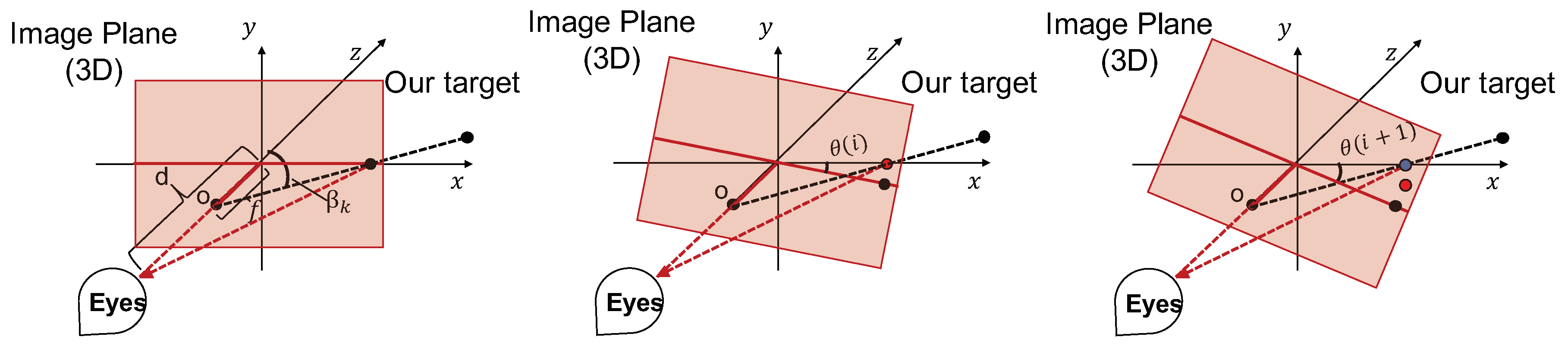
Figure 5.
Example of .
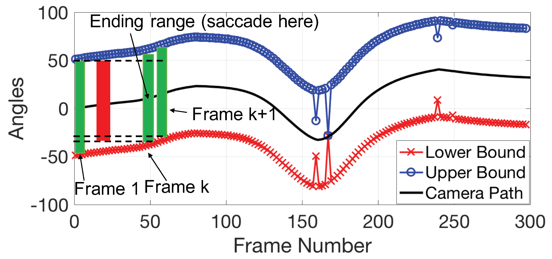
Figure 6.
of zero motion and motion with slope.

Figure 7.
Properties of First-Person Motion.

Figure 8.
Example of a First-Person Motion.
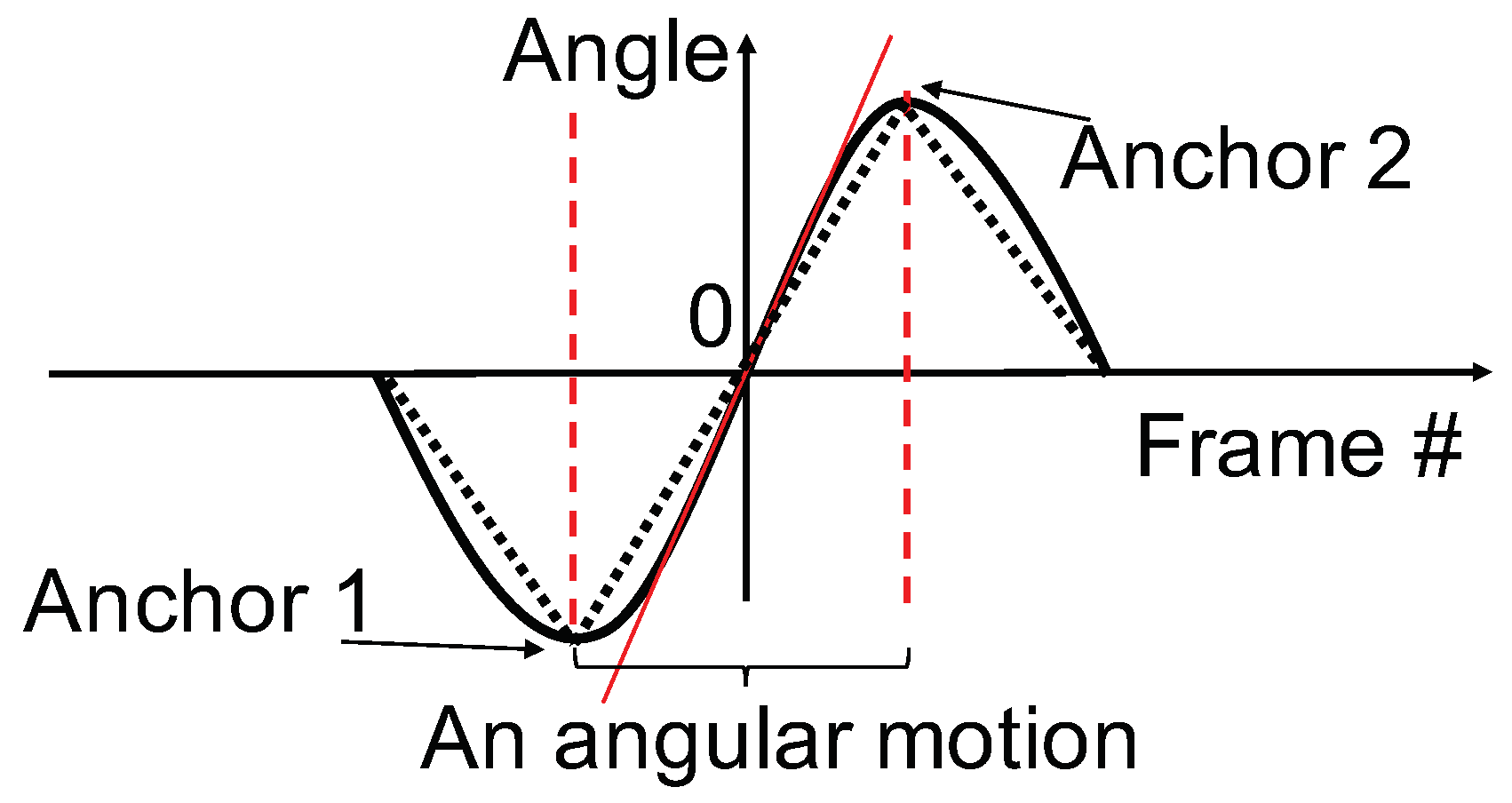
Figure 9.
Viewing Experience (VE) scores based on pure motions. (a) Example of pure motion; (b) VE scores.
Figure 9.
Viewing Experience (VE) scores based on pure motions. (a) Example of pure motion; (b) VE scores.

Figure 10.
General procedure of motion editing.
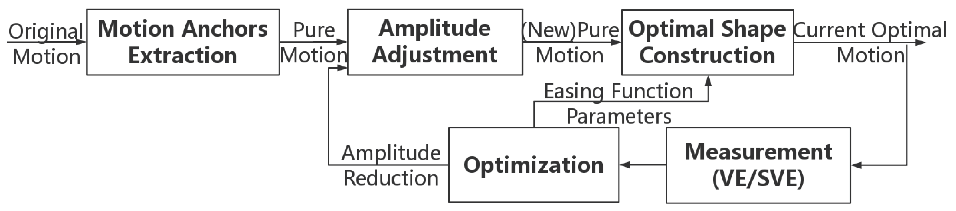
Figure 11.
Example of the VE score of a FPV.

Figure 12.
Suggested threshold to achieve under different motion frequencies and viewing distances.

Figure 13.
Example frames of source videos: (a) lobby; (b) market; (c) university street (US); (d) park walkway (PW).
Figure 13.
Example frames of source videos: (a) lobby; (b) market; (c) university street (US); (d) park walkway (PW).
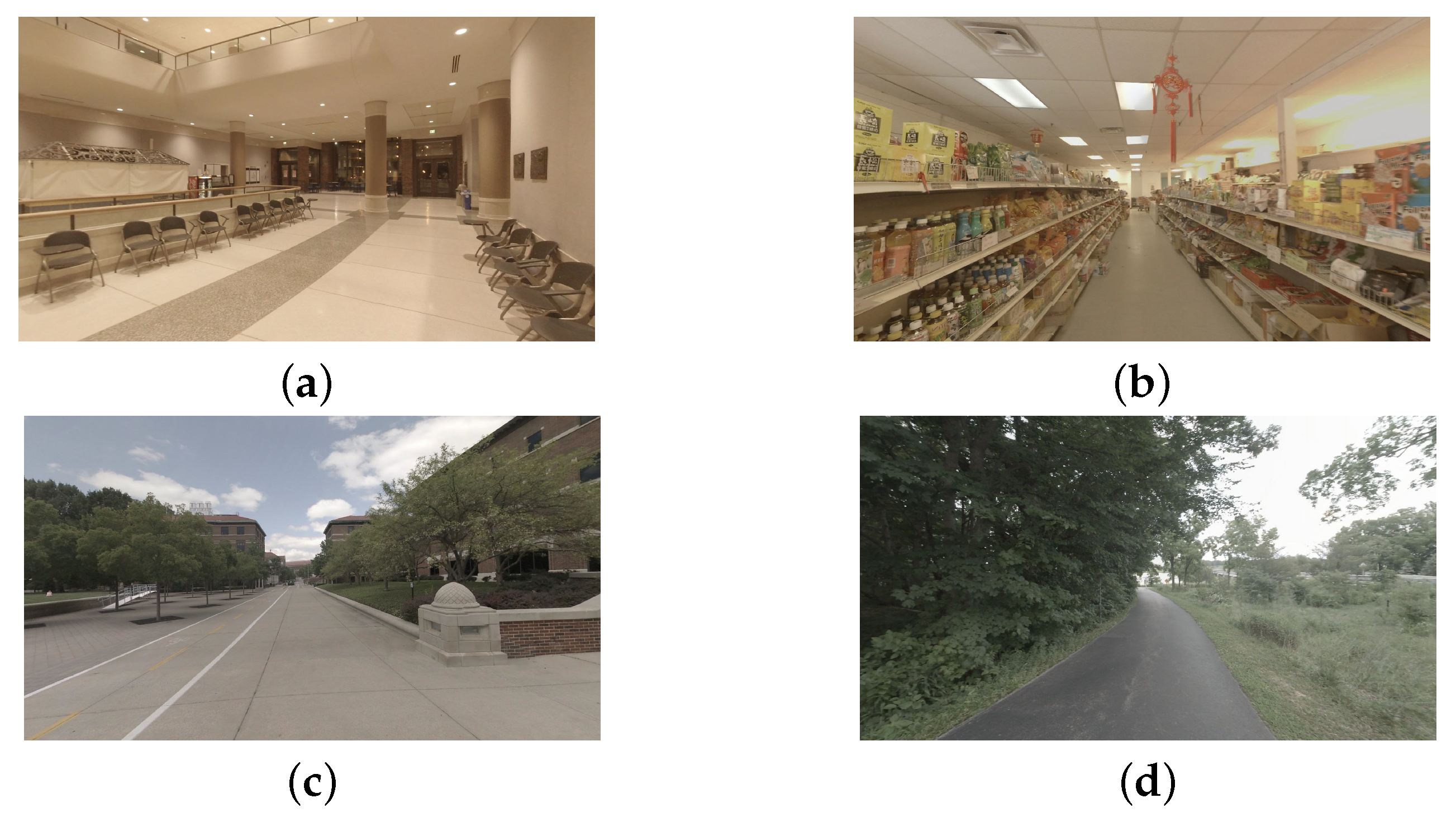
Figure 14.
Average Pearson linear correlation coefficient (PLCC) values across four test scenes under different bias parameters and the standard deviations under different bias settings.
Figure 14.
Average Pearson linear correlation coefficient (PLCC) values across four test scenes under different bias parameters and the standard deviations under different bias settings.

Figure 15.
Error caused by synthetic motions.
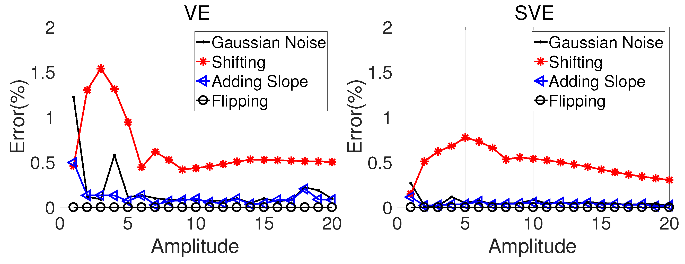
Figure 16.
Result comparison of different version videos.


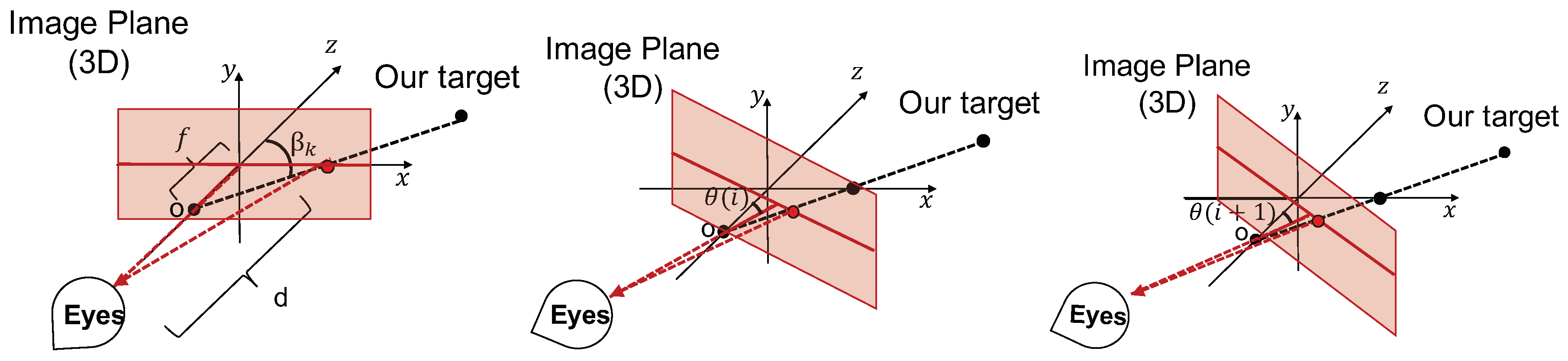
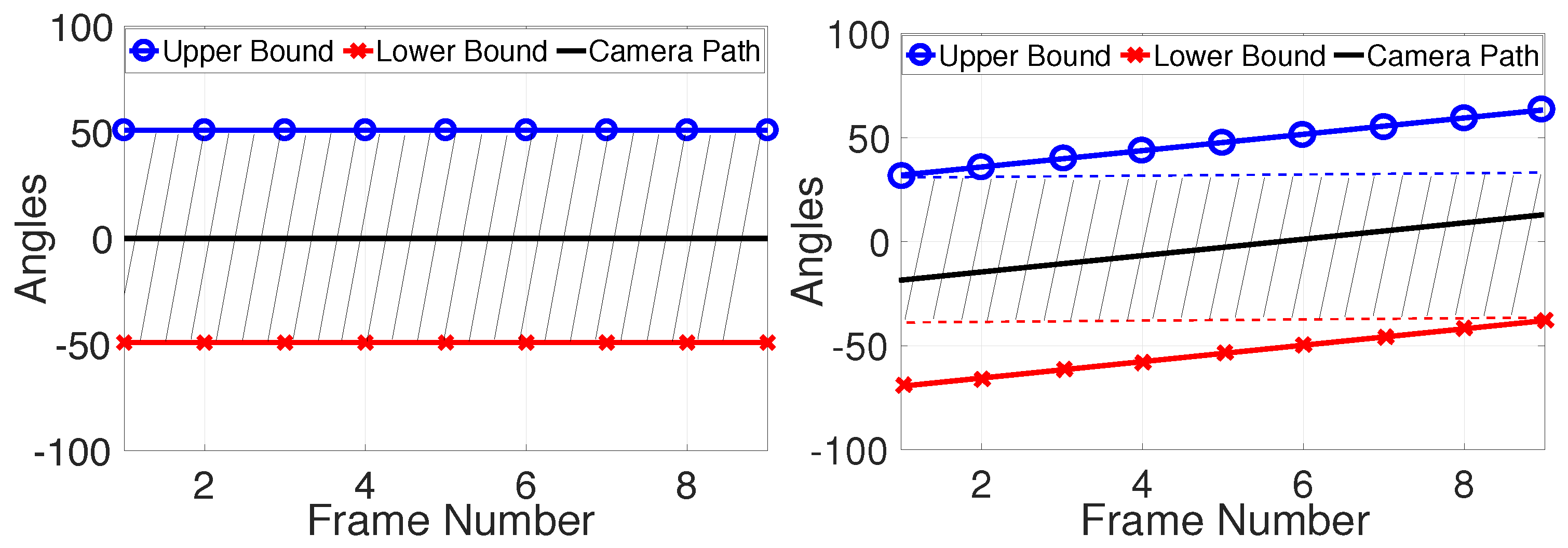
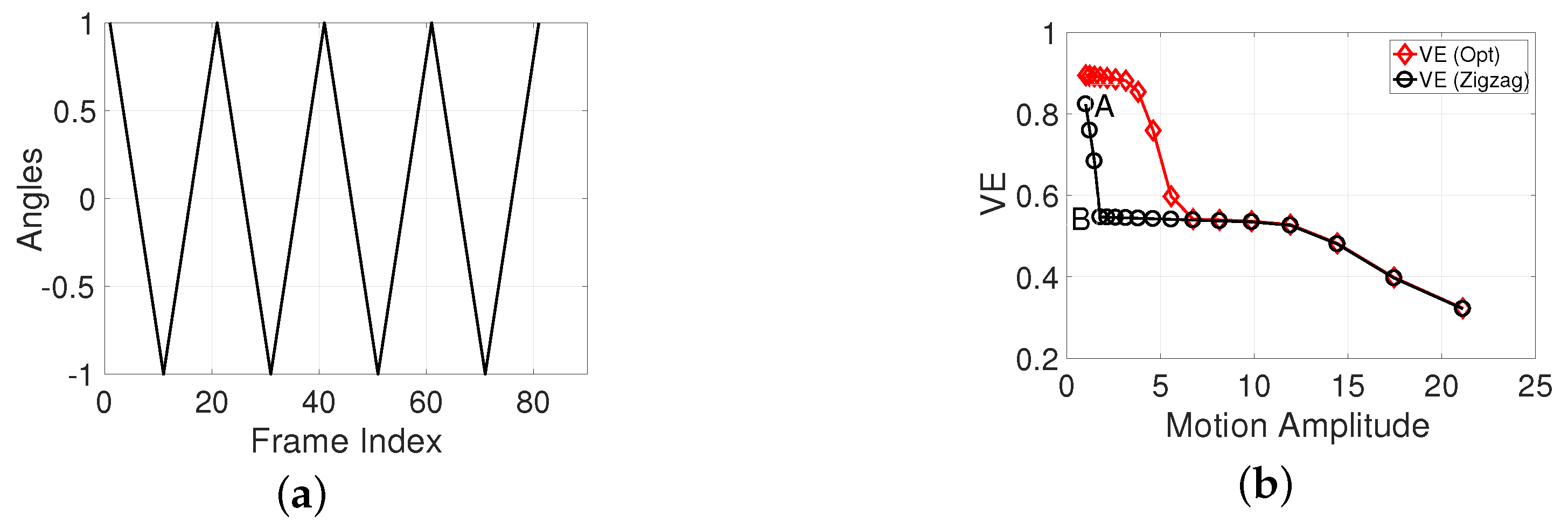
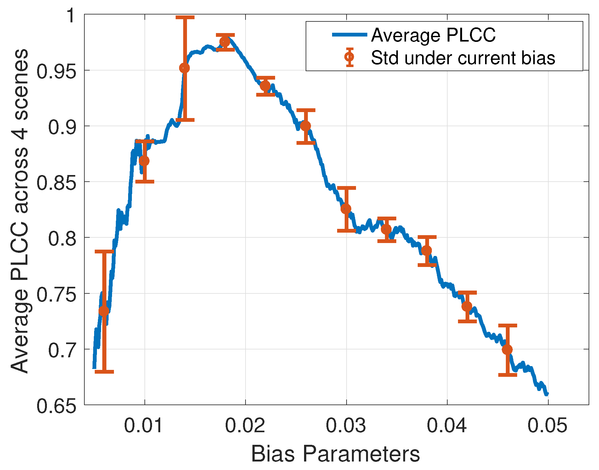
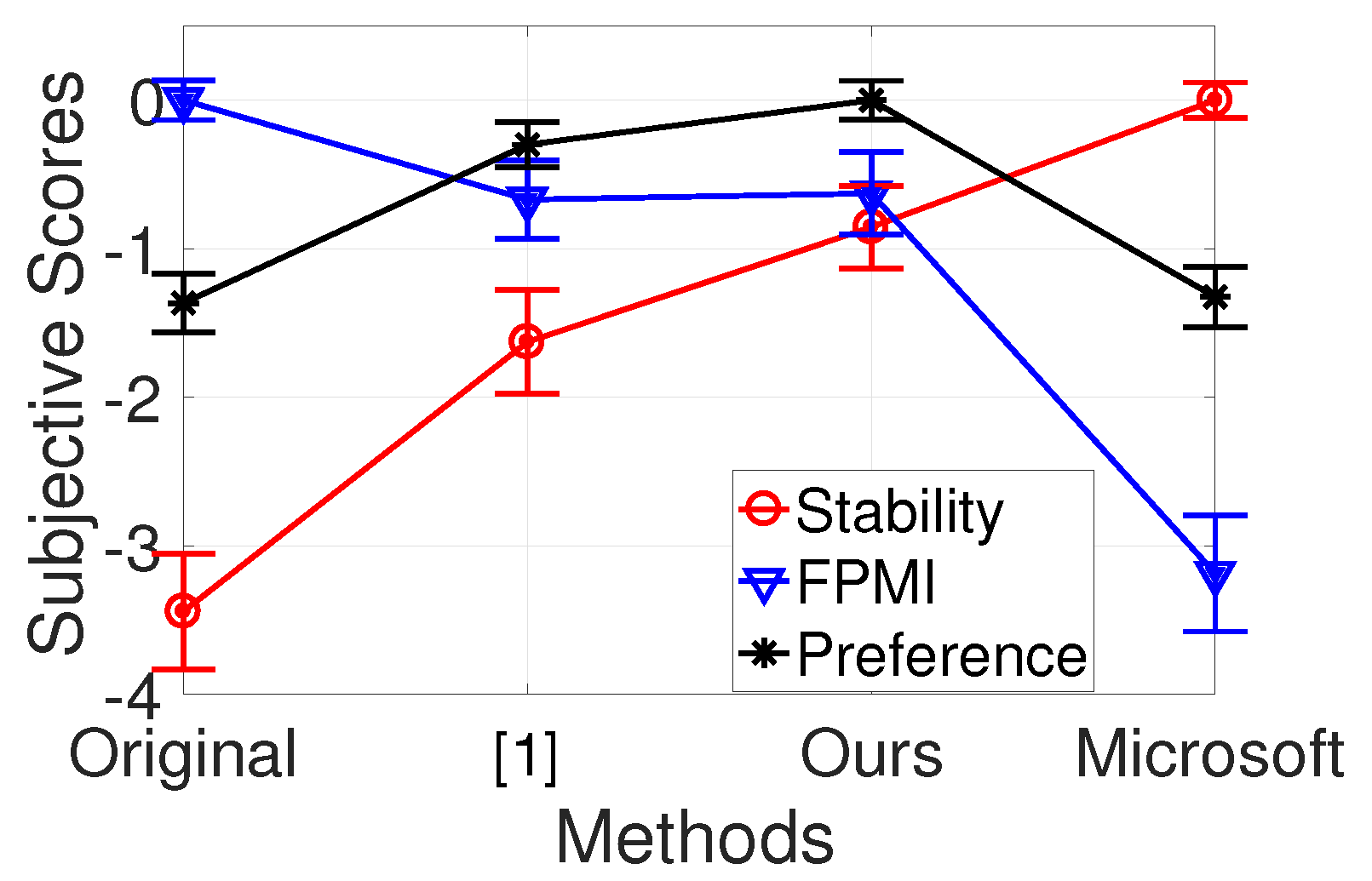
Table 1.
Concept Abbreviations.
| Abbreviations | Extend Names |
|---|---|
| FPVs | First-Person Videos |
| FPM | First-Person Motion |
| FPF | First-Person Feeling |
| FPMR | First-Person Motion Range |
| FPMI | First-Person Motion Information |
Table 2.
Bradley–Terry scores of all videos.
| Yaw Motion Amplitude | ||||||
|---|---|---|---|---|---|---|
| 4.3 | 6.2 | 8.1 | 10 | |||
| Lobby | 1.075 | 0 (0.345) | −3.057 (0.422) | −5.105 (0.550) | ||
| 1.55 | −4.027 (0.533) | −5.987 (0.622) | −7.813 (0.809) | |||
| 2.025 | −6.464 (0.652) | −9.021 (0.956) | ||||
| 2.5 | −9.857 (1.095) | |||||
| Market | 1.075 | 0 (0.387) | −1.262 (0.431) | −2.184 (0.495) | ||
| 1.55 | −1.268 (0.468) | −2.683 (0.555) | −4.445 (0.720) | |||
| 2.025 | −3.199 (0.580) | −4.906 (0.799) | ||||
| Pitch Motion Amplitude | 2.5 | −5.298 (0.870) | ||||
| US | 1.075 | 0 (0.370) | −3.057 (0.463) | −5.041 (0.588) | ||
| 1.55 | −3.734 (0.551) | −5.761 (0.671) | −7.087 (0.796) | |||
| 2.025 | −6.948 (0.763) | −7.981 (0.897) | ||||
| 2.5 | −8.641 (1.006) | |||||
| PW | 1.075 | 0 (0.434) | −1.885 (0.468) | −3.202 (0.515) | ||
| 1.55 | −2.083 (0.455) | −3.792 (0.566) | −5.101 (0.658) | |||
| 2.025 | −4.530 (0.624) | −5.950 (0.729) | ||||
| 2.5 | −6.516 (0.827) | |||||
Table 3.
Fraction of Correct Distance Conditions.
| VE | |||||
| Conditions | Cdn (41) | Cdn (42) | Cdn (43) | Cdn (44) | Total |
| Stability | 1 | 1 | 1 | 0.8 | 0.95 |
| FPMI | 0.8 | 1 | 1 | 0.8 | 0.9 |
| SVE | |||||
| Conditions | Cdn (41) | Cdn (42) | Cdn (43) | Cdn (44) | Total |
| Stability | 1 | 1 | 1 | 0.6 | 0.9 |
| FPMI | 0.8 | 1 | 1 | 0 | 0.7 |
Table 4.
Original inter-frame transformation fidelity (ITF) scores.
| Orig | Ours | Ours (Only Stabilization) | HL | DS | [5] | [6] | |
|---|---|---|---|---|---|---|---|
| Yard | 29.2 | 33.5 (0.6%) | 33.6 (1.28%) | 33.7 | 33.7 (17.2%) | 32.9 | 34.9 (37.0%) |
| Cave | 29.3 | 33.6 (0.03%) | 33.8 (0.05%) | 33.8 | 33.8 (7.3%) | 33.5 | 34.1 (7.8%) |
| Beach | 26.6 | 30.3 (0.74%) | 30.4 (1.2%) | 30.9 | 30.9 (15.5%) | 30.5 | 30.8 (10.0%) |
| Climb1 | 28.0 | 32.7 (0.5%) | 32.9 (4.98%) | 32.6 | 32.6 (19.0%) | 32.3 | 33.2 (22.6%) |
| Climb2 | 28.4 | 32.4 (0.76%) | 32.4 (0.31%) | 33.6 | 33.6 (13.0%) | 32.3 | 33.0 (13.4%) |
| Average | 28.3 | 32.5 (0.5%) | 32.6 (1.56%) | 32.9 | 32.9 (14.4%) | 32.3 | 33.2 (18.2%) |
© 2018 by the authors. Licensee MDPI, Basel, Switzerland. This article is an open access article distributed under the terms and conditions of the Creative Commons Attribution (CC BY) license (http://creativecommons.org/licenses/by/4.0/).
Share and Cite
MDPI and ACS Style
Ma, B.; Reibman, A.R. Viewing Experience Model of First-Person Videos. J. Imaging 2018, 4, 106. https://doi.org/10.3390/jimaging4090106
AMA Style
Ma B, Reibman AR. Viewing Experience Model of First-Person Videos. Journal of Imaging. 2018; 4(9):106. https://doi.org/10.3390/jimaging4090106
Chicago/Turabian StyleMa, Biao, and Amy R. Reibman. 2018. "Viewing Experience Model of First-Person Videos" Journal of Imaging 4, no. 9: 106. https://doi.org/10.3390/jimaging4090106
Note that from the first issue of 2016, this journal uses article numbers instead of page numbers. See further details here.