Partition and Inclusion Hierarchies of Images: A Comprehensive Survey


1
Lincoln Centre for Autonomous Systems Research, University of Lincoln, Lincoln LN6 7TS, UK
2
Univ. Rennes I, UMR 6074 IRISA, Campus de Beaulieu, 35042 Rennes, France
3
Univ. Bretagne Sud, UMR 6074, IRISA, F-56000 Vannes, France
*
Author to whom correspondence should be addressed.
†
These authors contributed equally to this work.
J. Imaging 2018, 4(2), 33; https://doi.org/10.3390/jimaging4020033
Submission received: 3 December 2017
/
Revised: 22 January 2018
/
Accepted: 25 January 2018
/
Published: 1 February 2018
(This article belongs to the Special Issue Computer Vision and Pattern Recognition)
Abstract
:The theory of hierarchical image representations has been well-established in Mathematical Morphology, and provides a suitable framework to handle images through objects or regions taking into account their scale. Such approaches have increased in popularity and been favourably compared to treating individual image elements in various domains and applications. This survey paper presents the development of hierarchical image representations over the last 20 years using the framework of component trees. We introduce two classes of component trees, partitioning and inclusion trees, and describe their general characteristics and differences. Examples of hierarchies for each of the classes are compared, with the resulting study aiming to serve as a guideline when choosing a hierarchical image representation for any application and image domain.
1. Introduction
Properties such as accuracy, size and relation between elements are considered for an image representation in accordance with the application domain. We list several such families of representations with their characteristics:
- Block-based representations (on binary images [3,4,5] and grayscale images [6,7,8]) divide the image into the set of (rectangular) arrays of pixels. It has fewer elements than pixel-based representations, but the image data are still not interpreted. Most common applications include image compression [3,6,7], segmentation [5,6], and feature and attribute extraction [4,5,8].
- Compressed (or frequency) domain representations store the image as a set of coefficients in a transform domain, such as Fourier transform [9,10], wavelets [10,11,12], ridgelets [13], contourlets [14], etc. Typical uses include image compression [10,11], denoising [13,15], reconstruction [12], texture analysis and segmentation [16]. Their advantage is a reduced image size, but they are sensitive to translation, rotation and scaling [17] and make it difficult to manipulate localized image content.
- Region-based representations group similar connected pixels using a segmentation algorithm, typically producing an over-segmentation. The resulting regions are often called superpixels [18], with the region adjacency information kept in a region-adjacency graph (RAG) [19] or combinatorial maps [20]. Different approaches include normalized cuts [21], graph-based segmentation by Felzenszwalb and Huttenlocher [22] and watershed segmentation [23,24], with a comparison in [18]. The reduced number of regions based on interpreting image information keeps the representational accuracy [2], but further unions of regions need to be considered to detect semantic structures [25].
- Hierarchical representations propose those most likely unions of regions on different scales of the image, from fine to coarse [25]. They enrich the horizontal relations between regions present in (partial) segmentations [26,27] with vertical inclusion information between regions at different scales. Initially, they were used for image filtering [2,28,29], segmentation [30,31,32] and boundary detection [33] but have since been applied to a vast amount of domains and applications (cf. Table 3).
We focus on the hierarchical representations of image in this work, and refer to them as component trees due to their aim to propose complex regions corresponding to “meaningful” image objects [28,29]. While hierarchical image representations have been receiving increasing amounts of attention [34,35,36] in image processing community, the structure, properties and construction of such hierarchies are the focus of study of Mathematical Morphology. Quad-trees [32,33] were amongst the first developed hierarchical image representations. However, they are regular hierarchies with predefined image division which is not dependent on the image content, and are in the same relation to the hierarchies considered in this paper as the block-based to the region-based representations. Recently, many different such hierarchical representations have been developed: Trees of Shapes [37,38,39], Binary Partition Trees (BPT) [2,25] and trees based on them (e.g., BPT by Altitude Ordering [40], Hierarchies of Minimum Spanning Forests [41]), -trees [42,43] and constrained connectivity hierarchies, such as -trees [42,44] which merit a structured study and comparison.
Contributions. The “building blocks” of hierarchical image representations were thoroughly investigated by Serra [26] and Ronse [27], who study the (partial) segmentations and partitions, and further the lattices of those (partial) partitions forming hierarchies [45,46,47]. In contrast to these and other theoretical works from Mathematical Morphology presented in a more general framework (e.g., [48]) and appropriated for different domains, we examine the component trees built directly from monochannel images represented by vertex-valued graphs and equipped with a 4-connectivity.
This paper formalizes the general characteristics of hierarchical representations, and introduces two distinct superclasses based on the common properties of the currently used representations (inclusion and partitioning trees, briefly introduced in [49]). While hierarchies provide the information relating to the image structure in terms of object relations, they need to be indexed in order to study the scale of image content. We present a consistent way of indexing the hierarchies based on dendrograms [50], and additionally propose a mapping from indexed inclusion hierarchies onto partitioning hierarchies on a doubled domain. Different hierarchies are compared in terms of structure, duality, parameterization, their ability to represent objects, and representation completeness.
Existing surveys covering several hierarchical informations are presented in the next section, followed by the basic notions used throughout the article in Section 3. Section 4 formalizes the hierarchies and proposes a unifying hierarchy classification and indexing, while Section 5 is dedicated to a detailed analysis of different hierarchies and their characteristics. A comparison between the current construction algorithms, including references, serving as user guidelines when making an implementation choice is given in Section 6. Finally, Section 7 offers a summary and comparison of different characteristics presented in Section 5 and Section 6, as well as identifies the open challenges based on the presented concepts, while the work will be concluded in Section 8.
2. Related Work
Despite the recent popularity of hierarchical image representations, the published works summarizing and comparing their characteristics tend to be limited to either a specific domain or hierarchy type. In contrast, we aim to explain the general properties of popular hierarchical representations and their behavior in different domains such as filtering, segmentation and object detection.
Hierarchies are often used to select a specific or optimal image (partial) partition for further processing [51]. Partitions and partial partitions are constituent parts of hierarchical representations, studied in the unifying papers by Serra [26] and Ronse [27] which present the theory of (partial) partitions and study the lattices they make and their relations. The hierarchies are studied and formally defined in [45] as an erosion from the lattice of levels to that of partial partitions. In contrast to our proposition to study the hierarchy structure and scale separately, the definition of a hierarchy offered by Ronse [45] refers directly to indexed hierarchy. We offer both definitions for each studied hierarchy in order to facilitate their use in the theoretical framework of Ronse [45], further expanded to study the ordering between partitions forming hierarchies [46,47].
Soille [42] examined multiple approaches to hierarchical image partitioning, focusing on the problems caused by the chaining effect in the -hierarchy and proposing constrained connectivity solutions. The studied hierarchies are compared in the context of image simplification, comparing the number of regions based on simplification strength (level) as well as visually comparing the segmentation results. Although the paper proposes many potential modifications to -connectivity, presently, only the global range constraints are widely used, forming a hierarchy known as -tree.
An exhaustive survey of filtering tools called connected operators was offered by Salembier and Wilkinson [52], focusing on their characteristics and techniques used to create them, and encompassing both the “classical” filtering approaches based on pixel-based representations as well as the approaches based on component trees. Approaches based on simplifying component trees with pruning and non-pruning strategies act on the connected components where the image is constant, bridging the gap between filtering and segmentation. Several hierarchies are presented in the strong context of filtering. It deals with extrema-oriented filtering based on inclusion trees, complemented only by a Binary Partition Tree for regions of intermediate level and without focusing on the implications of replacing an inclusion hierarchy with a partitioning one.
In contrast, the paper by Najman and Soille [44] formalizes the structure of hierarchical partitioning representations in the context of image segmentations, extending on the definitions of hierarchical clustering while taking spatial relations between the image elements into account. The ultrametric property of hierarchical clustering is explained in the context of hierarchical segmentations, emphasizing the importance of object scale. Hierarchies are represented by dendrograms [50], and the ultrametric watershed is introduced as a new visualization and computation scheme for partitioning hierarchies. We extend the framework to inclusion hierarchies, but regard the structural information of a component tree separately from the scale information in an indexed hierarchy.
One of most recent surveys, by Cousty et al. [40], is presented in the framework of edge-weighted graphs (i.e., operating on the dissimilarities between image pixels, as opposed to working directly with pixel values). It is accompanied by a paper which presents efficient quasi-linear algorithms based on the Kruskal Minimum Spanning Tree algorithm for computing these hierarchies [53], and establishes the relations between the -tree of an image with other Mathematical Morphology hierarchies and segmentation from markers. Recently, these links were studied further in [54] and put additionally in relation with saliency maps, images which can be interpreted as characteristic maps of hierarchies used for visualization, accompanied by example applications both from the field of image analysis and outside of it.
An application independent survey paper was presented by Najman and Cousty [55] covering a larger scope of morphological image processing techniques. It presents the basic concepts in modern Mathematical Morphology, offering introductory discussions on several topics. They discuss in detail different connectivities which can be used to define the image graph as well as the basic morphological operators. Image segmentation and connected filtering techniques leading to hierarchies of partitions are also presented through examples linking the -tree hierarchy, minimum spanning forests and watersheds on edge-valued graphs, offering an intuitive insight into various image processing tasks performed on hierarchies. Contrary to this work, which presents the reader with different choices of connectivity relations and filtering criteria but only provides a general idea of the capabilities of hierarchical image processing, our work uses a straightforward framework of 4-connectivity in order to better emphasize the differences and properties of hierarchies under examination.
The published surveys are mostly application-dependent, deal with a limited range of hierarchical representations and do not contrast well the hierarchies of partitions and partial partitions. The goal of this paper will thus be to provide an application independent reference about the structure and characteristics of commonly used hierarchical representations, decoupling the structure of the hierarchy from the scale of the represented regions. It is aimed at a general image processing audience, as a guide in comparing a large range of different hierarchical representations and aid when making a choice of representation.
3. Image Representation
This section describes the primary definitions from graph theory following [56], explains the interpretation of images as graphs and finally defines the terminology used in Mathematical Morphology to refer to image components. Firstly, in Section 3.1, we revise how images, partitions and regions are represented on a graph. Secondly, in Section 3.2, we define further terminology for handling image regions, as well as some characteristic image regions.
3.1. Images as Graphs
A graph comprises points and arrows which join one point to another. More formally, a graph is an ordered pair , where V denotes a set of points, called vertices (or nodes) and U a family of arrows between those points (i.e., duplicate elements are allowed), called arcs. Two vertices joined by an arc are said to be adjacent. An edge is obtained from an arc by discarding the direction of said arc. If the directions of arcs between the vertices are not specified, it is more convenient to represent the graph as a pair , where E stands for the set of edges, and such a graph is then referred to as an undirected graph. An undirected graph is a simple graph if it has no loops (edges from a vertex to itself) and has no more than one edge between any two vertices. While all results applicable to undirected and directed graphs can be applied to both types of graphs indiscriminately, for convenience, it is easier to distinguish between the two types depending on the application. Further, let I be a grayscale digital image which comprises a set of pixels, and , where is the set of natural numbers including 0. A function that assigns to each pixel its intensity value. The dual image, denoted by , comprises the same set of pixels while the intensity function is changed: , where is the maximum allowed gray level.
When representing an image I as a graph, the image pixels correspond to the set of vertices V, and choosing an adjacency relation or connectivity (cf. [1] for more details on connectivity and [57,58,59,60] for examples of advanced connectivities) determines the set of edges E connecting those pixels and associates an undirected graph to the image. An edge between two adjacent pixels p and q is denoted by or . When using regular 4-connectivity, we can distinguish the image boundary pixels as those pixels that do not have the full set of 4 neighbors. For a theoretical analysis of connectivity and connections, the theory of connective segmentation [26] and its extension to partial connections [27] permit combining different connections.
A path in from to is defined by a sequence of vertices (pixels) such that for all the pixels and are adjacent. A path from to is a cycle if and has no duplicate edges. denotes the set of all possible paths in between any p and q. Pixels p and q are connected in if and only if there is a path in from p to q or if .
We next define the concepts involved into image segmentation based tasks. A subgraph of generated by a set of vertices is defined as , where . A partial graph of is generated by a set of edges and defined as (i.e., all the vertices and a selected set of edges from the original graph.) Finally, we denote a partial subgraph of by , and define it as a subgraph of a partial graph, . Such is said to be connected if all are connected in .
A region of I generated by a nonempty is defined by , . A connected region or a connected component of the image I is a region which is connected and of maximal extent, i.e., . For a region , one can similarly define connected components as connected regions of maximal extent. We denote the set of all connected components of the image as , or a region as . Unless explicitly specified, all the partial subgraphs and regions in the remainder of the article will be connected.
A set of regions is said to partition the image if it covers the entire image domain and the elements of the set are mutually disjoint:
It can be also defined through an equivalence relation or by associating each point to a class [26,61]. The intensity function is partitioned using one of many existing image segmentation algorithms [26]. The regions need not be connected (i.e., segmentation to foreground and background, into predetermined classes [62,63,64], second generation connectivity [57,65]). However, in case of simple 4-connectivity, one would typically work with connected components of the regions for the purpose of building the component trees from the regions.
A segmentation can also determine boundaries between the regions, or contain a residual. If the region set returned by an algorithm does then not cover the entire image domain and is not a partition, it can be handled in the framework of partial partitions introduced by Ronse [27]. Similar to Equation (1), the elements of the set partially partition the image if they are disjoint, but need not cover the image domain. In fact, the set:
is called the support of the partial partition, and partitions the image on its support . Both the family of partitions and family of partial partitions of a set form a complete lattice, with the ordering between partitions given by:
This relation defines the refinement order on partitions, and an equivalent relation defined between any two partial partitions and gives the standard order. The greatest element of the lattices is the partition into one region containing the whole set, while the smallest element is the empty partition for the lattice of partial partitions, and a partition into singleton elements for the lattice of partitions. The lattices are studied in detail in [26,27].
3.2. Manipulating Image Components
A region boundary of a region is defined as the set of edges given by:
The sets of pixels of the inner and outer boundary are then made out of all the end-points of the boundary edges that belong (resp. do not belong) to the region :
All the image pixels not belonging to a connected region ( but ) make a set of 0 or more connected regions of maximal size in the image domain I, . If a does not contain any image boundary pixels, it is called a hole of the region (cavity in case of 3D images). The operation of filling all the holes of a connected region, , adds all the pixels contained in all the holes of a region to that region :
Flat zones of the image are connected components of the image I on the partial subgraph of generated by the set of edges such that , that is connected regions of maximal size comprised only of pixels at the same gray level [66,67]. Flat zone at a gray level k can be described as:
We call a flat zone of the image a local maximum if it is surrounded by pixels of strictly lower gray level:
Local minima are flat zones surrounded by pixels of strictly higher gray level. Local minima and local maxima together make the local extrema of the image.
The upper and lower level sets ( and , respectively) of an image are sets of image pixels with gray level values higher or lower than k:
We additionally define , and as subgraphs generated by , respectively, while still referring to them as flat zones or level sets of the image, and note that they each comprise several connected components.
4. Component Trees
This section provides a framework for the definition and indexing of hierarchies as well as highlights the construction differences between two types of hierarchies. First, Section 4.1 recalls the definitions of hierarchies on partitions and partial partitions following the formalization in [45,46]. Then, Section 4.2 highlights practical construction differences and region evolution within typical hierarchies, classifying them into partitioning and inclusion hierarchies. Finally, we describe the framework for indexing such hierarchies in Section 4.3 according to the specificities of the two classes.
4.1. Hierarchies of Partitions and Partial Partitions
Partitions and partial partitions form lattices, defined by the refinement order for partitions, or the standard order (containing the merging, inflating and inclusion orders) for partial partitions (cf. [46] for a detailed study on these orders). Thus, in morphological image segmentation a hierarchy is typically defined as an increasing sequence of (partial) partitions going from the least to the greatest element of the lattice: , where the least element is (partition to singletons) for partitions and (empty partition) for partial partitions [46,68]. In practice, all the non-singleton regions at the hierarchy bottom can be treated as singleton elements.
However, the definition through a sequence of (partial) partitions does not decouple the shape and inclusion information from the scale inposed on the regions by indexing (i.e., assigning levels to) the hierarchy. We define a hierarchy without indexing it, similarly to [69]:
- ,
- for each two elements the following holds: or .
Elementary regions do not need to be included, which allows the support of the partial partition to grow through the hierarchy. This definition imposes the partial ordering on the regions only, contrary to the one through a sequence of (partial) partitions imposing an order on the partitions building the hierarchy. In fact, any set of regions for which these rules hold defines a hierarchy, as we are only interested in the unique hierarchy components. We further justify it by the fact that in case of selecting optimal image segmentation from a hierarchy, one needs to consider the regions of the hierarchy separately rather than the (partial) partitions building it (studied in [2,70,71] with the most recent unifying theory by Kiran and Serra [51,72]). It corresponds to selecting optimal cuts in the hierarchies based either on externally imposed criteria (i.e., energy imposed to partitions) [51,70] or ground truth images [72,73].
To model the structure of a hierarchy, we deal with what berge [56] called arborescences or rooted trees, which are defined on directed graphs. In directed graphs, the arcs are ordered pairs of elements and an arc from n to m does not imply the existence of . A quasi-strongly connected graph is such a graph where for every pair of vertices there exists a vertice r such that there is a path from r to p and from r to q, and a rooted tree is a quasi-strongly connected acyclic graph. The definition of a path in a tree and a graph is similar, except that the arcs have to be directed for all consecutive elements . If there exists an arc in a tree, m is called the parent of n and n a child of m. The vertex m is called an ancestor of n if there exists a path in from m to n. The only node which has no children in is called the root of the tree, while the nodes that have no children are called leaf nodes. Let be a set of nodes. C is a cut of the tree if every path from the root to any leaf passes through exactly one node .
In a tree which is a component tree, the nodes of the tree model the regions of the hierarchy and the arcs model their inclusion. The region represented by a node is denoted by . The root node corresponds to the whole image, while leaf nodes are such nodes for which . A hierarchy shown in Figure 1a is modeled by the component tree in Figure 1b.
The relation between the parent region and the regions represented by its children can be formalized as follows. If m is a parent node in the tree and are all the children of m, the following rules describe how to construct m from its children:
where
The edge set of the parent can be represented as:
and the pixel set has to be such that the following holds:
Equation (12) states that a pixel set of the parent can be written as a union of the pixel sets of all its children, and optionally a set of additional pixels . Equation (15) ensures the connectedness of the resulting union, and Equation (14) that is indeed a region with the vertex set . This describes the rules one needs to follow when constructing tree regions in a bottom-up approach.
To reconstruct an image from the associated component tree, an altitude or model needs to be assigned to each node n which introduces new pixels into the hierarchy, i.e., which is a leaf, or for which . When forming an image, gray level is assigned to all pixels as they are introduced to the hierarchy, at the altitude of the corresponding node. Scale information is imposed by indexing the hierarchy, discussed in Section 4.3. an indexed hierarchy corresponds to the definition through a sequence of (partial) partitions.
We also note that an extension to the framework of hierarchies of (partial) partitions has been proposed by Kiran and Serra [74] through introducing braids of partitions. A braid is a family of partitions larger than a hierarchy, such that the pairwise supremum of any two partitions of the braid forms a cut in some monitoring hierarchy . A single braid can posses multiple monitoring hierarchies, while any hierarchy is a braid with itself as a monitor. By definition, dynamic programming properties valid on hierarchies are still valid on braids of partitions. Braids of partitions are a tool allowing to combine and fuse multiple hierarchies calculated on different modes of a multimodal image. This structure however lies outside of the framework of partitions and partial partitions [46] (and in fact extends it), as it is more than a hierarchy. As such, further discussion exceeds the scope of this paper and the interested reader is referred to [74,75] for the theory of braids of partitions, and to [76] for their application to multimodal image segmentation. We also direct the reader interested in combining different hierarchies of the same image into a new hierarchy (rather than a braid or some other structure) to [54] where such a method was proposed for the hierarchies of partitions.
4.2. Construction Differences between Inclusion and Partitioning Hierarchies
Equations (12)–(15) are general relations formalizing the hierarchy through a component tree. While the hierarchies are naturally divided into hierarchies of partitions and those of partial partitions, in current literature the hierarchies of partial partitions tend to be further restricted. We propose the names of partitioning trees for the hierarchies on the lattice of partitions, and inclusion trees for the subset of the hierarchies on the lattice of partial partitions, based on the nature of parent–child relations in the representations. Such a categorization was previously proposed in [49] and is explored here in more detail with added illustrations and explanations Any hybrid superclasses would necessarily be hierarchies of partial partitions. an example would be hierarchies of quasi-flat-zones or -connected components constrained by minimal area threshold (the authors thank one of the reviewers for this example.) However, to the best of our knowledge, all the currently studied and used hierarchies can be assigned into one of the two proposed superclasses. This difference between the classes is shown in Figure 2.
Inclusion trees. The leaf nodes of inclusion trees hold small regions or points, such as local image maxima or minima [28,29,37], or markers on the image [77]. In a typical bottom-up construction, nodes are formed by a region growing process starting from the leaves by adding one or more pixels (in Mathematical Morphology, this commonly means the image flat zones) to the existing regions. The new node becomes a parent of the nodes merged by this action and this continues until the root node is obtained covering the whole image domain. As the regions are only formed by adding new pixels to existing region(s), we constrain Equation (13) to a strict inequality, .
Basic image simplification or filtering [52] using an inclusion tree includes cutting branches from the leaves up to a region satisfying a desired criterion and collapsing all the removed regions into their closest surviving ancestor. Inclusion trees in literature are based on gray level or contrast between regions, and as such model dark and bright image structures. In this case, the filtering removes small contrasted structures in the image without changing the larger structures.
Partitioning trees. The principal difference with inclusion trees is that the leaves, as well as any cut, of a partitioning tree forms an image partition [70]. The initial partition can be any oversegmentation of the image such as image pixels, flat zones [25,42] or watershed segmentation [78]. New regions of the inner nodes are formed as unions of two or more existing adjacent regions. To reflect this, a constraint is added to Equation (12) and to Equation (13).
At the core of the partitioning tree construction are the notions defining iterative merging [2], introduced by Garrido et al. [30]:
- Region model defines how regions and their unions are represented. It reflects the characteristics of the regions used in the construction process.
- Merging criterion or similarity (or dissimilarity) measure describes the interest of possible merges. It is based on the region model.
- Merging order defines the rules used to merge the regions and which merge to perform next based on the merging criterion.
Simplifying or filtering an image using a corresponding partitioning tree corresponds to selecting a cut in the tree based on some criterion and assigning a model (or altitude) to each node in the selected cut to be used in image reconstruction. As partitioning trees are not typically extrema-oriented and can represent regions of intermediate gray levels, filtering the tree removes the small variations in the gray levels of regions perceived as uniform.
4.3. Indexing the Hierarchy
A component tree defines any hierarchy through its structure. To fully exploit the scale and semantic information provided by the different construction algorithms, the hierarchy is indexed by assigning an attribute , called the level (of aggregation), to each node of the component tree. It is always a non-negative function of the nodes, increasing along each branch from the leaves towards the root, meaning that if m is an ancestor of n, then . An indexed hierarchy corresponds to the definition [46] through an increasing sequence of (partial) partitions. It can be equivalently defined as an erosion from the lattice of levels to the lattice of (partial) partitions, with an adjoint dilation assigning a level to each region of the hierarchy. This definition is given alongside the definition through an indexed component tree for each presented hierarchy in Section 5 for comparison.
A distance on a set of elements is a function satisfying the conditions of non-negativity, , identity, , symetry, and triangular inequality, for any elements of the set. A distance is an ultrametric distance if it obeys an ultratriangular inequality, a constraint stronger than the triangular inequality: for any three elements of a set, , it is true that . A bijection between indexed partitioning trees and ultrametric distances [69,79,80] on the same set is established for the case where if and only if n is a leaf node. This is in accordance with the construction algorithms of different partitioning trees, which tend to assign the same attribute value (usually ) to all the leaf nodes. The levels induce an ultrametric distance on all the vertices of an image graph with a corresponding partitioning tree , which can be expressed as:
A distance between any two image elements from I is given by the smallest level of a node n in the hierarchy representing a region containing both image elements. Such indexed trees are represented in a form of a dendrogram [50] (introduced under the name taxonomic tree [81] for hierarchical clustering), with node height corresponding to the level assigned to it (cf. Figure 3).
For inclusion trees and hierarchies of partial partitions in general the identity and non-negativity constraints become . The dendrogram of an inclusion tree is more complicated as points can enter the support of the partial partition at levels above 0 [46], which needs to be indicated even when they are entering the support by the process of growing (inflating) an existing region. An example of such dendrogram is shown in Figure 4c.
Adding the corresponding sets as nodes at the lowest level of the hierarchy will allow us to construct a partitioning tree from an inclusion tree, however we will be unable to distinguish the original from the added singletons or reconstruct the original inclusion hierarchy. This is similar to the problem encountered in [27] when trying to represent an output of a segmentation algorithm producing a residual in the framework of connective segmentations and partitions: adding the residual to the representation by supplementing the partial partition with singletons does produce a full partition, but makes the residual indistinguishable from the original partition components, promoting the introduction of the framework of partial partitions [27]. To avoid the loss of information, we propose to uniquely map an inclusion tree onto a partitioning tree with a double image domain. We extend every pixel with a ghost pixel at the same gray level, connected only to the original pixel in the image. All the pixels and their ghost pixels form the leaves of the tree and partition the new domain. A ghost pixel merges into the hierarchy at the same level (in the same node) as its original pixel does, ensuring that every node in the tree is formed by merging two or more nodes. The singletons in the hierarchy correspond to the auxilary nodes present due to the ghost regions, making it possible to distinguish between them and the nodes of the original hierarchy. We can now impose an ultrametric distance on the nodes of this new hierarchy if we assign all the auxiliary nodes the level 0. To ensure for all other nodes, we add an arbitrary constant to the level assigned by the construction algorithm, and then Equation (16) also holds for indexed inclusion hierarchies. This mapping is of general interest as it allows applying techniques developed for partitioning trees with inclusion trees, e.g., the technique of [82] on combining several hierarchies of the same image, and in general processing the inclusion trees in the more common framework of multiscale segmentations.
5. Analysis of Tree Characteristics
This section reviews the tree representations frequently used in current literature, offering their definitions as well as examining, summarizing and comparing their characteristics. First, the trees from the inclusion tree superclass are listed, followed by partitioning trees. The most efficient algorithms suited for implementation will be mentioned in Section 6.
5.1. Min and Max-Trees
We first explain the concept and give examples for the Min-tree, followed by explaining the implications of the duality relation with the Max-tree. The Min-tree is an inclusion tree representing the dark structures in the image, based on lower level sets with the leaves corresponding to local image minima. A connected component of the level set not present in the level set makes a new node with a region , which either becomes:
- a parent node to all the previously constructed nodes at lower levels which are included in the region of the new node: , ; or
- a leaf node if it does not include the regions of any previous nodes.
At the highest gray level, there is only one connected component covering the whole domain and forming the root of the tree. The hierarchy corresponds to distinct connected components of the lower level sets: , shown in Figure 5b. The local minima of the dual image correspond to the local maxima of the original. Thus, considering the upper level sets of I or the lower level sets of the dual we obtain the dual Max-tree hierarchy, defined as . The Min-tree is suitable for manipulation of dark image structures, and the Max-tree of the bright ones. However, keeping both representations to handle both types of object simultaneously as the trees are redundant and ensuring consistency between them is difficult [83].
The connected components of form a partial partition of the image, , thus the map is an erosion from the lattice of levels to the lattice of partial partitions on the image defining the Min-tree. It assigns the level k to the connected component of forming a node in the hierarchy. The level k is also used as the altitude, carrying the information about the darkest region pixel. To index the Max-tree, the erosion and levels are defined using the dual image instead, example of which is shown in Figure 5d,e. The altitude of a node at level k is calculated as .
The structure was introduced by Salembier et al. [29] as a Max-tree and by Jones [28] as a component tree, which only differ in how the representation is stored [84]. More complex hierarchies based on these trees were developed to use with advanced connectivity relations, such as the Dual-Input Max-Tree for mask-based connectivity [57,65] and hierarchies for hyperconnectivity [59]. Min-trees have also been calculated on inclusion hierarchies instead of images, to perform filtering operations in shape spaces [85].
5.2. Tree of Shapes
The Tree of Shapes (ToS) is an inclusion tree combining the Min and Max-tree [37,86] to represent both bright and dark structures simultaneously. The leaves correspond to all the local extrema, while the node regions hold shapes, obtained by applying the hole filling operator on all connected components of the lower and upper level sets. We can thus define the ToS hierarchy as . These shapes are either nested or disjoint [38,87]. A node n is the parent of node m if there is no shape such that . For the original image in Figure 5a, the 5 distinct shapes obtained from upper and lower sets in Figure 6a,b is shown in Figure 6c, with the final hierarchy in Figure 6d. The ToS is a self-dual structure, as the sets of local minima and maxima as well as the upper and lower level sets are inverted in the dual image , which then produces the same ToS. The redundancy is eliminated by using the modified connected components (i.e., shapes) when combining the trees.
To index the Tree of Shapes and obtain the dendrogram in Figure 6e, we rely on the notion of dynamics along a path (introduced as a contrast measure [88]) and the notion of region dynamics. The dynamics along the path is defined as the sum of intensity differences of adjacent pixels along the path:
Region dynamics of a region is chosen between all minimal dynamics along the paths between pixels in the same branch of the tree, as the largest such path dynamic:
It can also be defined recursively:
which allows for easy level calculation in a bottom-up tree construction. The level of the node n associated to the region is then equal to the region dynamics of the region. To define the hierarchy as an erosion, we define the dynamic shapes at level k:
We also define as the subgraph generated by , and obtain the map as the erosion from the lattice of levels to the lattice of partial partitions indexing the ToS hierarchy. The ToS is a complete image representation, where the node altitudes correspond to the level h of the region from the upper or lower level set (resp. or ) which formed the shape , assigned to the node n. The altitude can be calculated from the levels if the gray levels of the leaves and the sign of the region dynamic for the inner nodes in Equation (19) are stored.
This type of structure was independently presented by Monasse and Guichard [86] for a combination of 4- and 8-connectivity, and by Song and Zhang [38] for 6-connectivity (proven equivalent in [89]). A reduced version of this hierarchy was also proposed by Song and Zhang [38,89], aiming to represent only the changes in the topology of the image. The name “Tree of Shapes”, used here, was chosen because it prevails in recent literature [39,83].
5.3. Binary Partition Tree
Binary Partition Tree (BPT) is a partitioning tree and is not extrema oriented [2], making it suited for representing objects with low, high and intermediate gray levels. The construction starts with assigning a node to each region from the initial partition which is based on pixels, flat zones or precomputed partitions [2,30]. The hierarchy depends on the choice of region model and merging criterion. The region model can be as simple as the average or median gray level of a region, and is typically assumed to be constant within a single region. A merging criterion is defined as a dissimilarity measure between the region models. The merging order used for the BPT is that of iterative region merging, and dictates the merging of the two regions most similar according to the merging criterion in each step (the order is not defined in the case of more than one pair of most similar regions). The merging sequence and the resulting tree for a BPT using a simple region model and criterion are shown in Figure 7.
The tree is not usually well balanced (cf. [2,25]) and can contain simple regions very close to the tree root. Thus, without any assumptions to the similarity measure used in merging, we propose an indexing in such a manner that the similarity measure of each merging step can always be recovered:
- if a node m of is a leaf node, then ,
- if a node m is created as a union of regions corresponding to the nodes and (i.e., ), and the dissimilarity between the regions in the moment of merging was , the level of the new node m is calculated according to:
A corresponding dendrogram for the tree in Figure 7e is shown in Figure 7f. The most precise reconstruction of the original image equals to the precision provided by the initial partition. While the self-duality of the BPT depends on the used region model and merging criterion (if based on gray or color level), it is typically desirable (the merging criterion used in Figure 7 is one such example). As the BPT is the most generic out of all the presented trees and does not pose any restrictions to the merging criterion, we only define the indexing of the nodes recursively due to the complexity of the closed-form solution as an erosion from the lattice of levels to the lattice of partitions.
The BPT is the most versatile hierarchy presented in this article, indroduced in Mathematical Morphology by Salembier and Garrido [2] by keeping track of the merging steps of iterative merging [30]. This work was continued in [25] by proposing a more suitable merging criterion and applying it to object detection, while the BPT and appropriate simplification methods were studied in [78]. Many developed extensions [41,53,90,91] highlight the relations to other component trees and morphological techniques, and specialize it according to the application domain. Additionally, many hierarchical representations outside of the morphological community fit well into the BPT framework, using segmentation methods such as watershed variants and Felzenszwalb-Huttenlocher segmentation to determine the initial partition, and defining the region models and similarity measures based on region boundary, color, texture, size and depth information [34,35,36]. We mention here the two notable specializations of the BPT, which have been used to produce hierarchies over images represented by edge-weighted rather than vertex-weighted graphs considered in this work.
Binary Partitioning Trees by Altitude Ordering establish the relation between min-trees (cf. Section 5.1) calculated on the edge graph of the image and -trees (cf. Section 5.4). They are an intermediate step in the calculation of the -tree (or quasi-flat-zone) hierarchy and other hierarchies when the edge values are calculated as the intensity differences between neighboring pixels, including additionally an imposed order between the edges of equal value, typically defined through Kruskal’s Minimum Spanning Tree algorithm [92]. Such a hierarchy was first explored by [93] where different segmentation methods based on the principal hierarchy were also proposed, as well as a possibility of different valuations of the graph edges. The concept was reintroduced to the community and formalized under the name of BPT by Altitude Ordering by Najman et al. [53] and Cousty et al. [54] where the relations to other hierarchies were established.
The Hierarchies of Minimum Spanning Forests establish the links with watersheds and segmentation from markers. They are also primarily defined on an edge-weighted graph of the image, but additionally require a set of markers ordered by importance. The markers are typically chosen as local minima of the weight map, when the MSF hierarchies correspond to watershed segmentation defined through the drop of water principle [24]. If the minima are additionally ordered by their extinction values [29,94] based on attributes such as area, depth or volume, the resulting Hierarchies of MSF are called hierarchical watersheds [41,54,77]. Hierarchies of MSF allow reordering of the hierarchy according to the calculated or perceived importance of minima, and have as such been used as 2D and 3D segmentation tools as well as for processing of geographical data [54].
5.4. -Tree
The second presented partitioning tree is the -tree. Unlike for the BPT, which relies on a predefined merging order but can be customized by the choice of initial partition, region model and merging criterion, all of these parameters are strictly defined for the -tree. We examine here the -tree for gray level images in detail, while the proposed adaptations for multichannel images will be discussed briefly in Section 7.2, along with other open challenges.
The initial partition in the -tree is always the partition to image flat zones. Using the notions introduced in Section 4.2 to describe the -tree, the region model, merging criterion and merging order are defined as follows:
- The region model for each region is the boundary of that region, .
- The merging criterion defines the similarity between two neighboring regions as the lowest edge (valued by gray level difference) common to models of both regions: .
- The merging order dictates that, in the i-th step, all regions with the similarity equal to i should be merged.
We also give a more natural definition through -connected components (also called quasi-flat zones). Image flat zones are considered as 0-connected components. To define the -connected components for some , the connected components are considered on the image graph where the neighboring pixels are connected if their gray level difference is less than or equal to . For increasing values of , these regions form a hierarchy represented by a tree. If we denote an -connected component to which a pixel p belongs to by , the hierarchical relation between the regions can be expressed as:
The -connected components for an image in Figure 8a are shown in Figure 8b–e, with the -tree shown in Figure 8f. To index the -tree (cf. example in Figure 8g) we define the quasi-flat-zone partition at level t as , and the map as the corresponding erosion from the lattice of levels to the lattice of partitions.
The locality of the similarity metric which considers only the neighboring pixels can cause gray level variations within a single region to be higher than expected for a certain . An example is shown in Figure 8f, where the level contains both a region with 18 and 2 pixels. This is referred to as the chaining effect and the extreme case is shown in Figure 9. Different approaches have been proposed to address this issue [42,44,95,96,97].
This tree is self-dual as the contrast information between neighboring pixels does not change in the dual image , and a complete image representation. Simplifying the images by approximating the regions in a partition formed by respecting a local range parameter was introduced in [98], studied further in [99], while the term -connected component was first used by Soille in [42,100] where the hierarchical properties of such regions were asserted.
5.5. -Tree
For the ease of understanding, we first provide the usual definitions of the -tree through the -connected components of maximal size, followed by the more complex definition through the region model, merging criterion and merging order. The -tree is a partitioning tree aiming to solve the problems with chaining effect present with -trees. If the parameter restricts the maximal range between locally connected pixels, corresponds to the maximal global gray level range inside a connected component. The global gray level range of a component is denoted by and is defined as the value difference between the highest and lowest pixel gray level value in the component. The notion of -connected components was introduced together with the notion of -connected components by Soille [100], denoted by for a pixel p, and defined as the with the maximal possible such that the global range is still lower or equal to :
Even though the following relation holds for every pixel p:
the set of all -connected components can not form a hierarchy due to the unknown order between and for and .
For , the local range parameter does not play a role, as the -connected components are equivalent to those for [42]. The are considered the largest with the global range less or equal to :
Unlike the components defined by Equation (23), the define a hierarchy, called the -tree. an example of this hierarchy for the image in Figure 8a is depicted in Figure 10.
To define the -tree through region model, region criterion and merging order, there are the following changes as when compared to the -tree:
- The region model for is the boundary of that region, , and minimal and maximal pixel values: .
- The merging criterion defines the similarity between all allowed sets of regions such that the subgraph of I generated by the union of all the region vertice sets: is connected. The weight of such a merge between a set of regions is:
- The merging order dictates that in the i-th step, all the sets of regions of maximal extent with the similarity equal to i should be merged.
Indexing the ()-tree is similar to indexing the -tree since they are both constrained connectivity hierarchies [42]: we define global range partitions as and as the corresponding erosion (cf. Figure 10g for dendrogram). The problems with the chaining effect are not completely solved since the -decomposition of the image can not contain regions not already present in the -decomposition, however the -indexing better reflects the region complexity (compare with for the full image in Figure 9c).
Since it is based on the -tree, the -tree retains its self-dual property and other characteristics. The -tree of the same image always has more levels, and the number of regions decreases more slowly from the leaf levels towards the root. However, as both trees represent only the unique regions, the -tree representation always has fewer nodes than the -tree since regions are removed from the -tree when forming an -tree. Both of these effects can be observed by comparing the dendrograms from Figure 8g and Figure 10g.
6. Construction Algorithms
We discuss here the approaches to construct various trees, explain the main idea behind each algorithm and provide the references to the original approaches. The complexity is expressed in relation to the number of image pixels N, depending on quantization defined by the number of bits used to code pixel values q and the range of those values .
Min- and Max-tree construction. a recent comparison of Min-tree and Max-tree construction algorithms was offered by Carlinet and Géraud [101], dividing the construction algorithms into immersion algorithms, flooding algorithms and merge-based algorithms. The merge-based approaches are mainly used for parallelism, and are not further discussed here (for a recent parallel implementation of Max-tree combining the merge-based and flooding approach, cf. e.g., [102]).
The first efficient Min-tree computation algorithm by Salembier et al. [29] is a flooding algorithm. It begins with the pixel at the gray level which constitutes a root pixel, from which the depth-first propagation through image elements is performed, recursively [29] or using a hierarchical queue [103]. For low quantization () a linear complexity of is achieved since k is small, but for larger q, the complexity becomes quadratic, , making them unsuitable for generic pixel (e.g., float) values. To overcome this, Wilkinson [65] replaces the hierarchical queue with a priority-queue, resulting in a flooding algorithm running in complexity for any pixel type with a total order (e.g., high dynamic range integers and float values).
The first step of immersion algorithms is sorting all the N image elements according to the appropriate order (i.e., the intensity ordering), which then form N disjoint singleton sets. Those sets are then merged to form a tree in the second step, using Tarjan’s union-find algorithm [104]. The complexity of the sorting step is bounded to for small integers (typically or ), but increases to for generic data types. For low quantized data, i.e., , the union-find implementations with lowest complexity by Berger et al. [84] and Najman and Couprie [105] use techniques such as root path compression, union-by-rank and level compression (to the detriment of memory usage) to achieve a quasi-linear time complexity of (—very slow growing inverse of the diagonal Ackermann’s function, ). For arbitrarily quantized data, the sorting step binds the complexity to .
Tree of Shapes construction. Early approaches to ToS construction operated with worst-case time complexity of [83,89] and were not easily extendible to multidimensional () images [37]. A recent algorithm by Géraud et al. [39] overcomes these drawbacks by using the immersion algorithms for Min-tree construction as a canvas, and replacing the sorting step.
The sorting step in an immersion algorithm should place the image elements from the external shapes before the elements from the internal shapes. For the ToS computation, representing the image as a set-valued map on a Kahlimsky grid [106] materializes the inter-pixel spaces and enables the computation of the correct shape order. The sorting step depends on a hierarchical queue, so can only handle quantized data, and runs in considered linear for low quantized data (authors recommend ). The immersion step has the same complexity as for the Min-tree, resulting in the quasi-linear complexity of for the whole algorithm.
Binary Partition Tree construction. The BPT computation starts with an initial partition, then merges the two most similar regions in each step (until reaching a single region), iteratively updating the similarity. We present here the complexity estimation of the construction algorithm for the case when updating the region model and calculating similarity between the models can be done in constant time, as studied by Guigues [107].
When no specific connectivity is imposed on the image, the iterative construction algorithm corresponds to hierarchical (agglomerative) clustering [108]. The detailed analysis of the algorithm identifies the advantages of using a hierarchical queue to keep the similarity information [30]. The initial partition is a segmentation into N separate pixels or regions. The similarities of the initial over-segmentation are sorted after calculation, which is bounded by for up to to similarities. The construction proceeds by iteratively finding the pair of most similar regions, removing the similarity information related to those regions, merging them and re-calculating the similarity information for the new region. Determining the smallest similarity is a constant operation in a hierarchical queue, while the similarities are updated in , with the number of iterations equal to the number of regions. Based on this, the construction complexity of BPT is bounded by . In the case of a specific connectivity, the speed of calculating and updating the similarity information can significantly decrease depending on the merging criterion used (4-connectivity analyzed in [109] approximates an upper bound to ). The special cases of BPT based on the -tree [40,53] can be constructed even faster, relying on their properties achieved by specializing the BPT parameters.
-tree construction. The -tree construction algorithm relies on its equivalence with a Min-tree defined on the edges valued with pixel intensity differences [44,69], and can use any Min-tree algorithm. Extending the idea, Havel et al. [110,111] calculate the -tree directly using a modification of Tarjan’s union-find [104], presenting an algorithm suited for multithreading applications.
The algorithm by Najman et al. [53], inspired by Kruskal’s Minimum Spanning Tree algorithm [92] and using Tarjan’s union-find [104], first constructs a BPT by Altitude Ordering, from which the -tree can be obtained with a linear post-processing step [40,53]. The complexity of the -tree construction algorithms is the same as for the Min-trees, and is quasi-linear in the number of image pixels for low quantization, .
()-tree construction. The first step in calculating the -tree and other constrained connectivity hierarchies is calculating the -tree they are based on. The ultrametric watersheds by Najman [69] enable visualizing these hierarchies and calculating them from the -tree based on the Lowest Common Ancestor (LCA) [112] in constant time for every pair of neighboring elements in the ultrametric watershed. The transformation into the -tree is itself linear.
The -tree can be interpreted as an -tree where the global component range is used as a region complexity measure according to Bosilj et al. [49], which proposes a filtering approach removing the nodes from the -tree and indexing the hierarchy by assigning the complexity measure as the level (of aggregation) to the nodes. This is realized by a bottom-up traversal of the tree, linear in the number of nodes of the tree and the number of image elements. Using any of the proposed approaches, the -tree can be constructed in the same complexity as the -tree, for low quantized image data.
7. Applications and Future Directions
This survey offers a comparison of component trees which is inclusive, not application-dependent and in the widespread image processing framework on vertex-valued graphs equipped with 4-connectivity. After the structure and the basic idea behind the construction algorithms of the trees were presented, this section focuses on current applications, interesting research directions and application domains for component trees. Section 7.1 offers an overview and comparison of the presented trees in terms of image processing applications, while the open challenges are outlined in Section 7.2.
7.1. Comparative Summary
For each tree, the characteristics such as duality, completeness and types of regions held in the representation were determined. The most basic choice is the one between inclusion trees and partitioning trees. While both types of hierarchies are well suited for image simplification, filtering and object detection, the structure of inclusion trees resulted in their common usage when selecting prominent image regions (such as discriminating keypoints) while the partitioning trees lend themselves better to producing segmentations of the image according to given criteria. As all the presented trees are complete representations, they can be either used directly as a search space, or their filtered versions or reduced hierarchies can be used if a smaller search space is needed.
The region types of different trees are closely examined as content representation has a direct influence on the type of objects and scenes each representation is well suited for. When working with extremal regions of the image, one should choose an inclusion tree representation. A choice between the different inclusion trees will depend on whether the contrast of the object related to the background is known in advance (for processing bright or dark objects, one would choose a Max-tree or a Min-tree respectively, but if this information is not known the ToS can be used to process both types of objects at the expense of slightly higher construction times). On the other hand, partitioning trees can contain regions at intermediate gray levels and are better suited for processing complex scenes (e.g., a satellite image of a whole city) and identifying composite objects. The most flexibility is offered by the BPT and its many specializations, where the construction parameters can be determined with a specific application in mind.
The construction complexity is another important factor to consider, and was examined for different quantization and data types in Section 6. All these characteristics are summarized for inclusion trees in Table 1 and partitioning trees in Table 2.
To provide a practical example of using these trees in image processing, a result of simple level-based filtering is shown in Figure 11. It shows the way different trees interact with image components, with the extrema-oriented inclusion trees processing the regions according to inclusion and gray-level order, and the partitioning hierarchies working on similarity-based regions with intermediate gray levels. On the one hand, a list of various application domains given in Table 3 shows that simplification, description of whole images (for remote and hyperspectral imaging) and, naturally, segmentation, are prevalent applications with partitioning trees. On the other hand, dealing with isolated image features (and applying them to image retrieval), as well as filtering out small details and noise, or segmenting and detecting specific objects on a contrasted background (e.g., in astronomical imaging) was mostly done using inclusion trees.
7.2. Open Challenges
Hereafter, we identify some open challenges not discussed herein, which would provide viable directions for future research.
This article focuses mainly on monochannel images, but as the examined hierarchical structures have a primary goal of providing good estimated locations of objects contained in the image, the color (and any other kind of) information contained in multichannel images has to be considered. For a general partitioning tree, working with vectorial instead of scalar image element values is fairly easy, as the total order between the values of image elements is not required. As such, the BPT was originally defined with color in mind [2], and the trend of including color information has persisted in current literature [25,78]. For the -tree, several adaptations for multichannel images exist [42,95,119,129,162] (https://github.com/pbosilj/trees-lib).
However, for the inclusion trees, due to a wide range of available total orderings on image element values [163] for multivariate data, this extension is not straightforward. Max-trees and Min-trees for multivariate data were first investigated for general applications [158]. The study of relations between these hierarchies and multivariate data in the context of connected filtering conducted by Passat and Naegel [164] and Kurtz et al. [159] define a more general structure called a component graph for multivalued images, as well as specific constraints under which a component graph preserves the tree structure and is instead referred to as multivalued component tree. An algorithm for extracting distinguished features from color images [165] also indirectly defines a Max-tree and Min-tree structure for color images. Extension of the Tree of Shapes to color images has been only very recently tackled by Carlinet and Géraud [166]. Let us note that when the tree is used solely for image description, processing multichannel data (e.g., hyperspectral images) can be simply achieved with a marginal strategy, i.e., building a tree for each image channel (see [141] for Max-trees and Min-trees, [63] for the Tree of Shapes), or by an hybrid marginal/vectorial strategy [152].
We also note advances in the application domain of image filtering where the Max-tree hierarchy was used to implement connected operators [29]. A whole variety of connected operators can be realized by replacing the Max-tree with other component trees, and this fundamental extension to the framework of connected operators was studied in [52]. Recently, Xu and co-authors [85,139] have proposed defining the filtering in shape space, an image whose adjacency relation is given by the parental relations in its original Max-tree. A novel way of filtering and node selection is also proposed by Perret and Collet [114], which puts Mathematical Morphology in relation with stochastic models, relying on a Markovian algorithm to classify the nodes of a tree.
Other open problems include finding the solution to the chaining effect present in -trees (cf. Subsec Section 5.4). This first led to defining logical predicate connectivity [100] and constrained connectivity [42,44,95,96,97,153] and establishing the -tree (explained in Section 5.5). More recently, mask-based connectivity, hyperconnectivity and directed connectivity, as well as the advanced hierarchies based on them [59,65,167], were introduced as a way to handle both visually disconnected objects, overlapping or weakly connected objects in images.
An interesting challenge would also be to formalize the theoretical relations between the hierarchies. They are only mentioned here as implied by the construction algorithms in Section 6. Examples include building the -trees as the Min-tree of the edges [69,110], representing the -tree as a BPT by imposing the order on its edges, and using the Max-tree algorithm as the canvas for the Tree of Shapes construction algorithm [39]. Relations between some other hierarchies have also been explicated in [40], but relations between all the hierarchies examined herein are still unknown and merit further examination.
8. Conclusions
We present a unifying survey of hierarchies of partitions and partial partitions used in practice, and propose a framework which decouples the structural shape information from the scale information added by indexing. The paper further offers a unifying view on the taxonomy and indexing of image hierarchies through component trees, which correspond naturally to the way the hierarchies are constructed and explicitly define the parent–child (inclusion) information between the regions. We propose two distinct categories of image hierarchies: inclusion and partitioning trees, and identify the restrictions to the general component tree formalization implied by the categories. The formalization through component trees can also be applied to potential new hybrid classes of trees by imposing different restrictions to the general definition. An established framework for indexing the hierarchies by dendrograms was described, which allows enriching the structural representation of the hierarchy with scale information. We propose a mapping from indexed inclusion trees to indexed partitioning trees, allowing us to recover the original inclusion tree.
We have presented the details, characteristics and construction algorithms of a large number of component trees, offering an application-independent way of comparing them, which makes it the most comprehensive such study thus far. The current growing interest in processing techniques interacting with image regions or superpixels rather than individual image elements and requiring a representation extending through multiple scales, often modeled as a hierarchy, make such a paper of particular interest.
Acknowledgments
The authors would like to thank Laurent Najman for fruitful discussions leading to presented indexing schemes for inclusion trees (and specifically for inspiration concerning Tree of Shapes indexing), and the anonymous reviewers for their constructive suggestions.
Author Contributions
This paper builds upon the doctoral work of Petra Bosilj, jointly supervised by Sèbastien Lefèvre and Ewa Kijak. Petra Bosilj designed and performed the experiments; Sèbastien Lefèvre and Ewa Kijak interpreted the findings. The article was co-written by the three authors.
Conflicts of Interest
The authors declare no conflict of interest.
References
- Soille, P. Morphological Image Analysis: Principles and Applications; Springer: Berlin, Germany, 2003. [Google Scholar]
- Salembier, P.; Garrido, L. Binary Partition Tree as an Efficient Representation for Image Processing, Segmentation, and Information Retrieval. IEEE Trans. Image Process. 2000, 9, 561–576. [Google Scholar] [CrossRef] [PubMed]
- Mohamed, S.; Fahmy, M. Binary Image Compression Using Efficient Partitioning into Rectangular Regions. IEEE Trans. Commun. 1995, 43, 1888–1893. [Google Scholar] [CrossRef]
- Flusser, J. Refined Moment Calculation Using Image Block Representation. IEEE Trans. Image Process. 2000, 9, 1977–1978. [Google Scholar] [CrossRef] [PubMed]
- Perantonis, S.; Gatos, B.; Papamarkos, N. Block decomposition and segmentation for fast Hough transform evaluation. Pattern Recognit. 1999, 32, 811–824. [Google Scholar] [CrossRef]
- Won, C. A Block-Based MAP Segmentation for Image Compressions. IEEE Trans. Circuits Syst. Video Technol. 1998, 8, 592–601. [Google Scholar]
- Chung, K.; Wu, J. Improved Image Compression using S-Tree and Shading Approach. IEEE Trans. Commun. 2000, 48, 748–751. [Google Scholar] [CrossRef]
- Chung, K.; Chen, P. An efficient algorithm for computing moments on a block representation of a grey-scale image. Pattern Recognit. 2005, 38, 2578–2586. [Google Scholar] [CrossRef]
- De Castro, E.; Morandi, C. Registration of Translated and Rotated Images Using Finite Fourier Transforms. IEEE Trans. Pattern Anal. Mach. Intell. 1987, 9, 700–703. [Google Scholar] [CrossRef] [PubMed]
- Vetterli, M.; Kovačević, J. Wavelets and Subband Coding; Prentice Hall PTR: Englewood Cliffs, NJ, USA, 1995. [Google Scholar]
- Mallat, S. A Theory for Multiresolution Signal Decomposition: The Wavelet Representation. IEEE Trans. Pattern Anal. Mach. Intell. 1989, 11, 674–693. [Google Scholar] [CrossRef]
- Lee, T. Image Representation Using 2D Gabor Wavelets. IEEE Trans. Pattern Anal. Mach. Intell. 1996, 18, 959–971. [Google Scholar]
- Do, M.; Vetterli, M. The Finite Ridgelet Transform for Image Representation. IEEE Trans. Image Process. 2003, 12, 16–28. [Google Scholar] [CrossRef] [PubMed]
- Do, M.; Vetterli, M. The Contourlet Transform: An Efficient Directional Multiresolution Image Representation. IEEE Trans. Image Process. 2005, 14, 2091–2106. [Google Scholar] [CrossRef] [PubMed]
- Mallat, S.; Hwang, W. Singularity Detection and Processing with Wavelets. IEEE Trans. Inf. Theory 1992, 38, 617–643. [Google Scholar] [CrossRef]
- Bovik, A.; Clark, M.; Geisler, W. Multichannel Texture Analysis Using Localized Spatial Filters. IEEE Trans. Pattern Anal. Mach. Intell. 1990, 12, 55–73. [Google Scholar] [CrossRef]
- Monasse, P. Morphological Representation of Digital Images and Application to Registration. Ph.D. Thesis, Paris-Dauphine University, Paris, France, 2000. [Google Scholar]
- Achanta, R.; Shaji, A.; Smith, K.; Lucchi, A.; Fua, P.; Süsstrunk, S. SLIC Superpixels Compared to State-of-the-Art Superpixel Methods. IEEE Trans. Pattern Anal. Mach. Intell. 2012, 34, 2274–2282. [Google Scholar] [CrossRef] [PubMed]
- Rosenfeld, A. Adjacency in digital pictures. Inf. Control 1974, 26, 24–33. [Google Scholar] [CrossRef]
- Lienhardt, P. Topological models for boundary representation: A comparison with n-dimensional generalized maps. Comput. Aided Des. 1991, 23, 59–82. [Google Scholar] [CrossRef]
- Shi, J.; Malik, J. Normalized cuts and image segmentation. IEEE Trans. Pattern Anal. Mach. Intell. 2000, 22, 888–905. [Google Scholar]
- Felzenszwalb, P.; Huttenlocher, D. Efficient graph-based image segmentation. Int. J. Comput. Vis. 2004, 59, 167–181. [Google Scholar] [CrossRef]
- Vincent, L.; Soille, P. Watersheds in digital spaces: An efficient algorithm based on immersion simulations. IEEE Trans. Pattern Anal. Mach. Intell. 1991, 13, 583–598. [Google Scholar] [CrossRef]
- Cousty, J.; Bertrand, G.; Najman, L.; Couprie, M. Watershed Cuts: Minimum Spanning Forests and the Drop of Water Principle. IEEE Trans. Pattern Anal. Mach. Intell. 2009, 31, 1362–1374. [Google Scholar] [CrossRef] [PubMed]
- Vilaplana, V.; Marques, F.; Salembier, P. Binary Partition Trees for Object Detection. IEEE Trans. Image Process. 2008, 17, 2201–2216. [Google Scholar] [CrossRef] [PubMed]
- Serra, J. A Lattice Approach to Image Segmentation. J. Math. Imaging Vis. 2006, 24, 83–130. [Google Scholar] [CrossRef]
- Ronse, C. Partial Partitions, Partial Connections and Connective Segmentation. J. Math. Imaging Vis. 2008, 32, 97–125. [Google Scholar] [CrossRef]
- Jones, R. Component trees for image filtering and segmentation. Comput. Vis. Image Underst. 1997, 75, 215–228. [Google Scholar] [CrossRef]
- Salembier, P.; Oliveras, A.; Garrido, L. Antiextensive Connected Operators for Image and Sequence Processing. IEEE Trans. Image Process. 1998, 7, 555–570. [Google Scholar] [CrossRef] [PubMed] [Green Version]
- Garrido, L.; Salembier, P.; Garcia, D. Extensive operators in partition lattices for image sequence analysis. Signal Process. 1998, 66, 157–180. [Google Scholar] [CrossRef]
- Meyer, F. an overview of morphological segmentation. Int. J. Pattern Recognit. Artif. Intell. 2001, 15, 1089–1118. [Google Scholar] [CrossRef]
- Horowitz, S.L.; Pavlidis, T. Picture segmentation by a tree traversal algorithm. J. ACM 1976, 23, 368–388. [Google Scholar] [CrossRef]
- Tanimoto, S.; Pavlidis, T. a hierarchical data structure for picture processing. Comput. Graph. Image Process. 1975, 4, 104–119. [Google Scholar] [CrossRef]
- Arbelaez, P.; Maire, M.; Fowlkes, C.; Malik, J. Contour detection and hierarchical image segmentation. IEEE Trans. Pattern Anal. Mach. Intell. 2011, 33, 898–916. [Google Scholar] [CrossRef] [PubMed]
- Hoiem, D.; Efros, A.A.; Hebert, M. Recovering occlusion boundaries from an image. Int. J. Comput. Vis. 2011, 91, 328–346. [Google Scholar] [CrossRef]
- Uijlings, J.R.; Van De Sande, K.E.A.; Gevers, T.; Smeulders, A.W.M. Selective search for object recognition. Int. J. Comput. Vis. 2013, 104, 154–171. [Google Scholar] [CrossRef]
- Monasse, P.; Guichard, F. Fast Computation of a Contrast-Invariant Image Representation. IEEE Trans. Image Process. 2000, 9, 860–872. [Google Scholar] [CrossRef] [PubMed]
- Song, Y.; Zhang, A. Monotonic tree. In Proceedings of the 10th International Conference, DGCI 2002, Bordeaux, France, 3–5 April 2002; Volume 2301, pp. 114–123. [Google Scholar]
- Géraud, T.; Carlinet, E.; Crozet, S.; Najman, L. A quasi-linear algorithm to compute the tree of shapes of nD images. In Proceedings of the 11th International Symposium, ISMM 2013, Uppsala, Sweden, 27–29 May 2013; Volume 7883, pp. 97–108. [Google Scholar]
- Cousty, J.; Najman, L.; Perret, B. Constructive Links between Some Morphological Hierarchies on Edge-Weighted Graphs. In Proceedings of the 11th International Symposium, ISMM 2013, Uppsala, Sweden, 27–29 May 2013; Volume 7883, pp. 85–96. [Google Scholar]
- Cousty, J.; Najman, L. Incremental Algorithm for Hierarchical Minimum Spanning Forests and Saliency of Watershed Cuts. In Proceedings of the 10th International Symposium, ISMM 2011, Verbania-Intra, Italy, 6–8 July 2011; Volume 6671, pp. 272–283. [Google Scholar]
- Soille, P. Constrained Connectivity for Hierarchical Image Partitioning and Simplification. IEEE Trans. Pattern Anal. Mach. Intell. 2008, 30, 1132–1145. [Google Scholar] [CrossRef] [PubMed]
- Ouzounis, G.; Soille, P. Pattern Spectra from Partition Pyramids and Hierarchies. In Proceedings of the 10th International Symposium, ISMM 2011, Verbania-Intra, Italy, 6–8 July 2011; Volume 6671, pp. 108–119. [Google Scholar]
- Najman, L.; Soille, P. On Morphological Hierarchical Representations for Image Processing and Spatial Data Clustering. In Applications of Discrete Geometry and Mathematical Morphology; Springer: Berlin/Heidelberg, Germany, 2012; Volume 7346, pp. 43–67. [Google Scholar]
- Ronse, C. Adjunctions on the lattices of partitions and of partial partitions. Appl. Algebr. Eng. Commun. Comput. 2010, 21, 343–396. [Google Scholar] [CrossRef]
- Ronse, C. Ordering partial partitions for image segmentation and filtering: Merging, creating and inflating blocks. J. Math. Imaging Vis. 2014, 49, 202–233. [Google Scholar] [CrossRef]
- Ronse, C. Orders for Simplifying Partial Partitions. J. Math. Imaging Vis. 2017, 58, 382–410. [Google Scholar] [CrossRef]
- Najman, L.; Meyer, F. A short tour of mathematical morphology on edge and vertex weighted graphs. In Image Processing and Analysis with Graphs; Lezoray, O., Grady, L., Eds.; CRC Press: Boca Raton, FL, USA, 2012; pp. 141–174. [Google Scholar]
- Bosilj, P.; Lefèvre, S.; Kijak, E. Hierarchical Image Representation Simplification Driven by Region Complexity. In Proceedings of the 17th International Conference, Naples, Italy, 9–13 September 2013; Volume 8156, pp. 562–571. [Google Scholar]
- Sokal, R.; Rohlf, F. The comparison of dendrograms by objective methods. Taxon 1962, 11, 33–40. [Google Scholar] [CrossRef]
- Kiran, B.R.; Serra, J. Global–local optimizations by hierarchical cuts and climbing energies. Pattern Recognit. 2014, 47, 12–24. [Google Scholar] [CrossRef] [Green Version]
- Salembier, P.; Wilkinson, M. Connected Operators. IEEE Signal Process. Mag. 2009, 26, 136–157. [Google Scholar] [CrossRef]
- Najman, L.; Cousty, J.; Perret, B. Playing with Kruskal: Algorithms for Morphological Trees in Edge-Weighted Graphs. In Proceedings of the 11th International Symposium, ISMM 2013, Uppsala, Sweden, 27–29 May 2013; Volume 7883, pp. 135–146. [Google Scholar]
- Cousty, J.; Najman, L.; Kenmochi, Y.; Guimarães, S. Hierarchical segmentations with graphs: quasi-at zones, minimum spanning trees, and saliency maps. J. Math. Imaging Vis. 2016. [Google Scholar] [CrossRef]
- Najman, L.; Cousty, J. a graph-based mathematical morphology reader. Pattern Recognit. Lett. 2014, 47, 3–17. [Google Scholar] [CrossRef]
- Berge, C. Graphs and Hypergraphs; North-Holland Publishing Company: Amsterdam, The Netherlands, 1973. [Google Scholar]
- Ouzounis, G.; Wilkinson, M. Mask-based second-generation connectivity and attribute filters. IEEE Trans. Pattern Anal. Mach. Intell. 2007, 29, 990–1004. [Google Scholar] [CrossRef] [PubMed]
- Ouzounis, G.; Wilkinson, M. Hyperconnected attribute filters based on k-flat zones. IEEE Trans. Pattern Anal. Mach. Intell. 2011, 33, 224–239. [Google Scholar] [CrossRef] [PubMed]
- Perret, B.; Lefèvre, S.; Collet, C.; Slezak, É. Hyperconnections and hierarchical representations for grayscale and multiband image processing. IEEE Trans. Image Process. 2012, 21, 14–27. [Google Scholar] [CrossRef] [PubMed] [Green Version]
- Ronse, C. Set-theoretical algebraic approaches to connectivity in continuous or digital spaces. J. Math. Imaging Vis. 1998, 8, 41–58. [Google Scholar] [CrossRef]
- Serra, J. Mathematical morphology for Boolean lattices. In Image Analysis and Mathematical Morphology, II: Theoretical Advances; Academic Press: Cambridge, MA, USA, 1988; pp. 37–58. [Google Scholar]
- Ghamisi, P.; Dalla Mura, M.; Benediktsson, J.A. a Survey on Spectral-Spatial Classification Techniques Based on Attribute Profiles. IEEE Trans. Geosci. Remote Sens. 2015, 53, 2335–2353. [Google Scholar] [CrossRef]
- Cavallaro, G.; Dalla Mura, M.; Benediktsson, J.A.; Bruzzone, L. Extended self-dual attribute profiles for the classification of hyperspectral images. IEEE Geosci. Remote Sens. Lett. 2015, 12, 1690–1694. [Google Scholar] [CrossRef]
- Damodaran, B.B.; Höhle, J.; Lefèvre, S. Attribute profiles on derived features for urban land cover classification. Photogramm. Eng. Remote Sens. 2017, 83, 183–193. [Google Scholar] [CrossRef]
- Wilkinson, M. a fast component-tree algorithm for high dynamic-range images and second generation connectivity. In Proceedings of the 18th IEEE International Conference on Image Processing (ICIP), Brussels, Belgium, 11–14 September 2011; pp. 1021–1024. [Google Scholar]
- Serra, J.; Salembier, P. Connected operators and pyramids. In Proceedings of the SPIE Image Algebra and Morphological Image Processing, San Diego, CA, USA, 11–16 July 1993; pp. 65–76. [Google Scholar]
- Salembier, P.; Serra, J. Flat zones filtering, connected operators, and filters by reconstruction. IEEE Trans. Image Process. 1995, 4, 1153–1160. [Google Scholar] [CrossRef] [PubMed]
- Meyer, F.; Najman, L. Segmentation, minimum spanning tree and hierarchies. In Mathematical Morphology: From Theory to Applications; Najman, L., Talbot, H., Eds.; Wiley: Hoboken, NJ, USA, 2010. [Google Scholar]
- Najman, L. On the Equivalence Between Hierarchical Segmentations and Ultrametric Watersheds. J. Math. Imaging Vis. 2011, 40, 231–247. [Google Scholar] [CrossRef] [Green Version]
- Guigues, L.; Cocquerez, J.P.; Le Men, H. Scale-sets image analysis. Int. J. Comput. Vis. 2006, 68, 289–317. [Google Scholar] [CrossRef]
- Serra, J. Hierarchies and Optima. Discrete Geometry for Computer Imagery, DGCI 2011; Debled-Rennesson, I., Domenjoud, E., Kerautret, B., Even, P., Eds.; Springer: Berlin/Heidelberg, Germany, 2011; Volume 6607. [Google Scholar]
- Kiran, B.R.; Serra, J. Scale space operators on hierarchies of segmentations. In ternational Conference on Scale Space and Variational Methods in Computer Vision; Springer: Berlin/Heidelberg, Germany, 2013; pp. 331–342. [Google Scholar]
- Kiran, B.R.; Serra, J. Ground truth energies for hierarchies of segmentations. In Proceedings of the 11th International Symposium, ISMM 2013, Uppsala, Sweden, 27–29 May 2013; Volume 7883, pp. 123–134. [Google Scholar]
- Kiran, B.R.; Serra, J. Braids of partitions. In Proceedings of the 12th International Symposium, ISMM 2015, Reykjavik, Iceland, 27–29 May 2015; Volume 9082, pp. 217–228. [Google Scholar]
- Serra, J.; Kiran, B.R. Constrained Optimization on Hierarchies and Braids of Partitions. In Proceedings of the 12th International Symposium, ISMM 2015, Reykjavik, Iceland, 27–29 May 2015; Volume 9082, pp. 229–240. [Google Scholar]
- Tochon, G.; Dalla Mura, M.; Chanussot, J. Segmentation of Multimodal Images based on Hierarchies of Partitions. In Proceedings of the 12th International Symposium, ISMM 2015, Reykjavik, Iceland, 27–29 May 2015; Volume 9082, pp. 241–252. [Google Scholar]
- Najman, L.; Schmitt, M. Geodesic saliency of watershed contours and hierarchical segmentation. IEEE Trans. Pattern Anal. Mach. Intell. 1996, 18, 1163–1173. [Google Scholar] [CrossRef]
- Lu, H.; Woods, J.; Ghanbari, M. Binary partition tree analysis based on region evolution and its application to tree simplification. IEEE Trans. Image Process. 2007, 16, 1131–1138. [Google Scholar] [CrossRef] [PubMed]
- Johnson, S. Hierarchical clustering schemes. Psychometrika 1967, 32, 241–254. [Google Scholar] [CrossRef] [PubMed]
- Jardine, C.; Jardine, N.; Sibson, R. The structure and construction of taxonomic hierarchies. Math. Biosci. 1967, 1, 173–179. [Google Scholar] [CrossRef]
- Sneath, P. The application of computers to taxonomy. J Gen. Microbiol. 1957, 17, 201–226. [Google Scholar] [CrossRef] [PubMed]
- Maia, D.S.; de Albuquerque Araujo, A.; Cousty, J.; Najman, L.; Perret, B.; Talbot, H. Evaluation of Combinations of Watershed Hierarchies. In Proceedings of the 13th International Symposium, ISMM 2017, Fontainebleau, France, 15–17 May 2017; Volume 10225, pp. 133–145. [Google Scholar]
- Caselles, V.; Monasse, P. Geometric Description of Images as Topographic Maps; Springer: Berlin/Heidelberg, Germany, 2009. [Google Scholar]
- Berger, C.; Géraud, T.; Levillain, R.; Widynski, N.; Baillard, A.; Bertin, E. Effective component tree computation with application to pattern recognition in astronomical imaging. In Proceedings of the IEEE International Conference on Image Processing, San Antonio, TX, USA, 16 September–19 October 2007; Volume 4, pp. IV-41–IV-44. [Google Scholar]
- Xu, Y.; Géraud, T.; Najman, L. Connected Filtering on Tree-Based Shape-Spaces. IEEE Trans. Pattern Anal. Mach. Intell. 2016, 38, 1126–1140. [Google Scholar] [CrossRef] [PubMed] [Green Version]
- Monasse, P.; Guichard, F. Scale-space from a level lines tree. J. Vis. Commun. Image Represent. 2000, 11, 224–236. [Google Scholar] [CrossRef]
- Ballester, C.; Caselles, V.; Monasse, P. The tree of shapes of an image. ESAIM Control Optim. Calc. Var. 2003, 9, 1–18. [Google Scholar] [CrossRef]
- Grimaud, M. New measure of contrast: The dynamics. In Proc. SPIE 1769, Proceedings of the International Society for Optics and Photonics: Bellingham, WA, USA, 1992; Gader, P.D., Dougherty, E.R., Serra, J.C., Eds.; SPIE: Bellingham, WA, USA; pp. 292–305.
- Song, Y. a topdown algorithm for computation of level line trees. IEEE Trans. Image Process. 2007, 16, 2107–2116. [Google Scholar] [CrossRef] [PubMed]
- Jalba, A.C.; Westenberg, M.A. a comparison of two tree representations for data-driven volumetric image filtering. In Proceedings of the 10th International Symposium, ISMM 2011, Verbania-Intra, Italy, 6–8 July 2011; Volume 6671, pp. 405–416. [Google Scholar]
- Vichik, A.; Keshet, R.; Malah, D. Self-dual morphology on tree semilattices and applications. In Proceedings of the 8th International Symposium on Mathematical Morphology, Rio de Janeiro, Brazil, 10–13 October 2007; Volume 10225, pp. 49–60. [Google Scholar]
- Kruskal, J. On the shortest spanning subtree of a graph and the traveling salesman problem. Proc. Am. Math. Soc. 1956, 7, 48–50. [Google Scholar] [CrossRef]
- Morris, O.; Lee, M.d.J.; Constantinides, A. Graph theory for image analysis: An approach based on the shortest spanning tree. Commun. Radar Signal Process. 1986, 133, 146–152. [Google Scholar] [CrossRef]
- Silva, A.; de Alencar Lotufo, R. New extinction values from efficient construction and analysis of extended attribute component tree. In Proceedings of the SIBGRAPI’08 XXI Brazilian Symposium on Computer Graphics and Image Processing, Campo Grande, Brazil, 12–15 October 2008; pp. 204–211. [Google Scholar]
- Soille, P.; Grazzini, J. Constrained Connectivity and Transition Regions. In Proceedings of the 9th International Symposium, ISMM 2009, Groningen, The Netherlands, 24–27 August 2009; Volume 5720, pp. 59–69. [Google Scholar]
- Soille, P. Constrained connectivity for the processing of very-high-resolution satellite images. Int. J. Remote Sens. 2010, 31, 5879–5893. [Google Scholar] [CrossRef]
- Soille, P. Preventing Chaining through Transitions While Favouring It within Homogeneous Regions. In Proceedings of the 10th International Symposium, ISMM 2011, Verbania-Intra, Italy, 6–8 July 2011; Volume 6671, pp. 96–107. [Google Scholar]
- Nagao, M.; Matsuyama, T.; Ikeda, Y. Region extraction and shape analysis in aerial photographs. Comput. Vis. Graph. 1979, 10, 195–223. [Google Scholar] [CrossRef]
- Meyer, F. The levelings. In Proceedings of the Fourth International Symposium on Mathematical Morphology and Its Applications to Image and Signal Processing, Amsterdam, The Netherlands, 3–5 June 1998; pp. 199–206. [Google Scholar]
- Soille, P. On genuine connectivity relations based on logical predicates. In Proceedings of the 14th International Conference on Image Analysis and Processing, Modena, Italy, 10–14 September 2007; pp. 487–492. [Google Scholar]
- Carlinet, E.; Géraud, T. a comparative review of component tree computation algorithms. IEEE Trans. Image Process. 2014, 23, 3885–3895. [Google Scholar] [CrossRef] [PubMed]
- Moschini, U.; Meijster, A.; Wilkinson, M. a Hybrid Shared-Memory Parallel Max-Tree Algorithm for Extreme Dynamic-Range Images. IEEE Trans. Pattern Anal. Mach. Intell. 2018, in press. [Google Scholar] [CrossRef] [PubMed]
- Nistér, D.; Stewénius, H. Linear time maximally stable extremal regions. In Proceedings of the 10th European Conference on Computer Vision, Marseille, France, 12–18 October 2008; Volume 5303, pp. 183–196. [Google Scholar]
- Tarjan, R.E. Efficiency of a good but not linear set union algorithm. J. ACM 1975, 22, 215–225. [Google Scholar] [CrossRef]
- Najman, L.; Couprie, M. Building the Component Tree in Quasi-Linear Time. IEEE Trans. Image Process. 2006, 15, 3531–3539. [Google Scholar] [CrossRef] [PubMed]
- Najman, L.; Géraud, T. Discrete set-valued continuity and interpolation. In Proceedings of the 11th International Symposium, ISMM 2013, Uppsala, Sweden, 27–29 May 2013; Volume 7883, pp. 37–48. [Google Scholar]
- Guigues, L. Modèles Multi-Échelles Pour la Segmentation D’images. Ph.D. Thesis, École Doctorale Sciences et Ingénierie, Cergy-Pontoise, France, 2003. [Google Scholar]
- Duda, R.; Hart, P.; Stork, D. Pattern Classification; Wiley: Hoboken, NJ, USA, 2000. [Google Scholar]
- Al-Dujaili, A.; Merciol, F.; Lefèvre, S. GraphBPT: An efficient hierarchical data structure for image representation and probabilistic inference. In Proceedings of the 12th International Symposium, ISMM 2015, Reykjavik, Iceland, 27–29 May 2015; Volume 9082, pp. 301–312. [Google Scholar]
- Havel, J.; Merciol, F.; Lefèvre, S. Efficient Schemes for Computing α-tree Representations. In Proceedings of the Mathematical Morphology and Its Applications to Signal and Image Processing, Uppsala, Sweden, 27–29 May 2013; Volume 7883, pp. 111–122. [Google Scholar]
- Havel, J.; Merciol, F.; Lefèvre, S. Efficient tree construction for multiscale image representation and processing. J. Real Time Image Process. 2016. [Google Scholar] [CrossRef]
- Bender, M.; Farach-Colton, M. The LCA problem revisited. In Proceedings of the 4th Latin American Symposium, Punta del Esk, Uruguay, 10–14 April 2000; Volume 1776, pp. 88–94. [Google Scholar]
- Westenberg, M.; Roerdink, J.; Wilkinson, M. Volumetric attribute filtering and interactive visualization using the max-tree representation. IEEE Trans. Image Process. 2007, 16, 2943–2952. [Google Scholar] [CrossRef] [PubMed]
- Perret, B.; Collet, C. Connected image processing with multivariate attributes: An unsupervised Markovian classification approach. Comput.Vis. Image Underst. 2015, 133, 1–14. [Google Scholar] [CrossRef] [Green Version]
- Kiwanuka, F.N.; Wilkinson, M.H.F. Automatic attribute threshold selection for morphological connected attribute filters. Pattern Recognit. 2016, 53, 59–72. [Google Scholar] [CrossRef]
- Xu, Y.; Géraud, T.; Najman, L. Morphological filtering in shape spaces: Applications using tree-based image representations. In Proceedings of the 2012 21st International Conference on Pattern Recognition (ICPR), Tsukuba, Japan, 11–15 November 2012; pp. 485–488. [Google Scholar]
- Carlinet, E.; Géraud, T. A Color Tree of Shapes with Illustrations on Filtering, Simplification, and Segmentation. In Proceedings of the 12th International Symposium, ISMM 2015, Reykjavik, Iceland, 27–29 May 2015; Volume 363–374, p. 9082. [Google Scholar]
- Xu, Y.; Géraud, T.; Najman, L. Hierarchical image simplification and segmentation based on Mumford–Shah-salient level line selection. Pattern Recognit. Lett. 2016, 83, 278–286. [Google Scholar] [CrossRef]
- Aptoula, E.; Weber, J.; Lefèvre, S. Vectorial quasi-flat zones for color image simplification. In Proceedings of the 11th International Symposium, ISMM 2013, Uppsala, Sweden, 27–29 May 2013; Volume 7883, pp. 231–242. [Google Scholar]
- Marcotegui, B.; Serna, A.; Hernández, J. Ultimate Opening Combined with Area Stability Applied to Urban Scenes. In Proceedings of the 13th International Symposium, ISMM 2017, Fontainebleau, France, 15–17 May 2017; pp. 261–268. [Google Scholar]
- Xu, Y.; Géraud, T.; Najman, L. Context-based energy estimator: Application to object segmentation on the tree of shapes. In Proceedings of the 2012 19th IEEE International Conference on Image Processing (ICIP), Orlando, FL, USA, 30 September–3 October 2012; pp. 1577–1580. [Google Scholar]
- Song, Y.; Zhang, A. Analyzing scenery images by monotonic tree. Multimed. Syst. 2003, 8, 495–511. [Google Scholar] [CrossRef]
- Cardelino, J.; Randall, G.; Bertalmio, M.; Caselles, V. Region based segmentation using the tree of shapes. In Proceedings of the 2006 IEEE International Conference on Image Processing, Atlanta, GA, USA, 8–11 October 2006; pp. 2421–2424. [Google Scholar]
- Igual, L. Image Segmentation and Compression Using the Tree of Shapes of an Image. Motion Estimation. Ph.D. Thesis, Pompeu Fabra University, Barcelona, Spain, 2006. [Google Scholar]
- Meyer, F. Minimum spanning forests for morphological segmentation. Math. Morphol. Appl. Image Process. 1994, 77–84. [Google Scholar] [CrossRef]
- Valero, S.; Salembier, P.; Chanussot, J. Comparison of merging orders and pruning strategies for binary partition tree in hyperspectral data. In Proceedings of the 2010 17th IEEE International Conference on Image Processing (ICIP), Hong Kong, China, 26–29 September 2010; pp. 2565–2568. [Google Scholar]
- Veganzones, M.; Tochon, G.; Dalla Mura, M.; Plaza, A.; Chanussot, J. Hyperspectral Image Segmentation Using a New Spectral Unmixing-Based Binary Partition Tree Representation. IEEE Trans. Image Process. 2014, 23, 3574–3589. [Google Scholar] [CrossRef] [PubMed] [Green Version]
- Tochon, G.; Feret, J.B.; Valero, S.; Martin, R.E.; Knapp, D.E.; Salembier, P.; Chanussot, J.; Asner, G.P. On the use of binary partition trees for the tree crown segmentation of tropical rainforest hyperspectral images. Remote Sens. Environ. 2015, 159, 318–331. [Google Scholar] [CrossRef] [Green Version]
- Merciol, F.; Lefèvre, S. Fast image and video segmentation based on alpha-tree multiscale representation. In Proceedings of the 2012 Eighth International Conference on Signal Image Technology and Internet Based Systems (SITIS), Naples, Italy, 25–29 November 2012. [Google Scholar]
- Merciol, F.; Lefèvre, S. Buffering hierarchical representation of color video streams for interactive object selection. In Proceedings of the 16th International Conference, ACIVS 2015, Catania, Italy, 26–29 October 2015. [Google Scholar]
- Tushabe, F.; Wilkinson, M. Image Preprocessing for Compression: Attribute Filtering. In Proceedings of the World Congress on Engineering & Computer Science, San Francisco, CA, USA, 24–26 October 2007. [Google Scholar]
- Solé, A.; Caselles, V.; Sapiro, G.; Arándiga, F. Morse description and geometric encoding of digital elevation maps. IEEE Trans. Image Process. 2004, 13, 1245–1262. [Google Scholar] [CrossRef] [PubMed]
- Urbach, E. Intelligent Object Detection Using Trees. In Proceedings of the 12th International Symposium, ISMM 2015, Reykjavik, Iceland, 27–29 May 2015; Volume 9082, pp. 289–300. [Google Scholar]
- Teeninga, P.; Moschini, U.; Trager, S.; Wilkinson, M. Improved Detection of Faint Extended Astronomical Objects Through Statistical Attribute Filtering. In Proceedings of the 12th International Symposium, ISMM 2015, Reykjavik, Iceland, 27–29 May 2015; Volume 9082, pp. 157–168. [Google Scholar]
- Benediktsson, J.A.; Bruzzone, L.; Chanussot, J.; Dalla Mura, M.; Salembier, P.; Valero, S. Hierarchical Analysis of Remote Sensing Data: Morphological Attribute Profiles and Binary Partition Trees. In Proceedings of the 10th International Symposium, ISMM 2011, Verbania-Intra, Italy, 6–8 July 2011; Volume 6671, pp. 306–319. [Google Scholar]
- Valero, S.; Salembier, P.; Chanussot, J. Object recognition in hyperspectral images using Binary Partition Tree representation. Pattern Recognit. Lett. 2015, 56, 45–51. [Google Scholar] [CrossRef] [Green Version]
- Tochon, G.; Chanussot, J.; Dalla Mura, M.; Bertozzi, A.L. Object Tracking by Hierarchical Decomposition of Hyperspectral Video Sequences: Application to Chemical Gas Plume Tracking. IEEE Trans. Geosci. Remote Sens. 2017. [Google Scholar] [CrossRef]
- Desolneux, A.; Moisan, L.; Morel, J.M. Edge detection by Helmholtz principle. J. Math. Imaging Vis. 2001, 14, 271–284. [Google Scholar] [CrossRef]
- Xu, Y.; Monasse, P.; Géraud, T.; Najman, L. Tree-based morse regions: A topological approach to local feature detection. IEEE Trans. Image Process. 2014, 23, 5612–5625. [Google Scholar] [CrossRef] [PubMed]
- Bosilj, P.; Kijak, E.; Lefèvre, S. Beyond MSER: Maximally Stable Regions using Tree of Shapes. In Proceedings of the Conference: British Machine Vision Conference 2015, Swansea, UK, 7–10 September 2015. [Google Scholar]
- Dalla Mura, M.; Benediktsson, J.A.; Waske, B.; Bruzzone, L. Extended profiles with morphological attribute filters for the analysis of hyperspectral data. Int. J. Remote Sens. 2010, 31, 5975–5991. [Google Scholar] [CrossRef]
- Bosilj, P.; Wilkinson, M.; Kijak, E.; Lefèvre, S. Local 2D Pattern Spectra as Connected Region Descriptors. Math. Morphol. Theory Appl. 2016. [Google Scholar] [CrossRef]
- Pham, M.; Aptoula, E.; Lefèvre, S. Feature profile from attribute filtering for classification of remote sensing images. IEEE J. Sel. Top. Appl. Earth Observ. Remote Sens. 2018, 11, 249–256. [Google Scholar] [CrossRef]
- Pham, M.; Aptoula, E.; Lefèvre, S. Local Feature-Based Attribute Profiles for Optical Remote Sensing Image Classification. IEEE Trans. Geosci. Remote Sens. 2018, in press. [Google Scholar] [CrossRef]
- Dalla Mura, M.; Benediktsson, J.A.; Bruzzone, L. Self-dual attribute profiles for the analysis of remote sensing images. In Proceedings of the 10th International Symposium, ISMM 2011, Verbania-Intra, Italy, 6–8 July 2011; Volume 6671, pp. 320–330. [Google Scholar]
- Bosilj, P.; Damodaran, B.; Aptoula, E.; Dalla Mura, M.; Lefèvre, S. Attribute Profiles from Partitioning Trees. In Proceedings of the 13th International Symposium, ISMM 2017, Fontainebleau, France, 15–17 May 2017; pp. 381–392. [Google Scholar]
- Gueguen, L.; Hamid, R. Toward a Generalizable Image Representation for Large-Scale Change Detection: Application to Generic Damage Analysis. IEEE Trans. Geosci. Remote Sens. 2016, 54, 3378–3387. [Google Scholar] [CrossRef]
- Tushabe, F.; Wilkinson, M. Content-based image retrieval using combined 2D attribute pattern spectra. In Proceedings of the 8th Workshop of the Cross-Language Evaluation Forum, Budapest, Hungary, 19–21 September 2007. [Google Scholar]
- Bosilj, P.; Aptoula, E.; Lefèvre, S.; Kijak, E. Retrieval of Remote Sensing Images with Pattern Spectra Descriptors. ISPRS In. J. Geo-Inf. 2016, 5, 228. [Google Scholar] [CrossRef]
- Aptoula, E. Remote Sensing Image Retrieval with Global Morphological Texture Descriptors. IEEE Trans. Geosci. Remote Sens. 2014, 52, 3023–3034. [Google Scholar] [CrossRef]
- Urbach, E.; Roerdink, J.; Wilkinson, M. Connected Shape-Size Pattern Spectra for Rotation and Scale-Invariant Classification of Gray-Scale Images. IEEE Trans. Pattern Anal. Mach. Intell. 2007, 29, 272–285. [Google Scholar] [CrossRef] [PubMed]
- Aptoula, E.; Dalla Mura, M.; Lefèvre, S. Vector attribute profiles for hyperspectral image classification. IEEE Trans. Geosci. Remote Sens. 2016, 54, 3208–3220. [Google Scholar] [CrossRef]
- Lefèvre, S.; Chapel, L.; Merciol, F. Hyperspectral image classification from multiscale description with constrained connectivity and metric learning. In Proceedings of the 2014 6th Workshop on Hyperspectral Image and Signal Processing: Evolution in Remote Sensing (WHISPERS), Lausanne, Switzerland, 24–27 June 2014. [Google Scholar]
- Merciol, F.; Lefèvre, S. Fast Building Extraction by Multiscale Analysis of Digital Surface Models. In Proceedings of the 2015 IEEE International Geoscience and Remote Sensing Symposium (IGARSS), Milan, Italy, 26–31 July 2015. [Google Scholar]
- Cavallaro, G.; Dalla Mura, M.; Benediktsson, J.A.; Plaza, A. Remote sensing image classification using attribute filters defined over the tree of shapes. IEEE Trans. Geosci. Remote Sens. 2016, 54, 3899–3911. [Google Scholar] [CrossRef]
- Aptoula, E. The impact of multivariate quasi-flat zones on the morphological description of hyperspectral images. Int. J Remote Sens. 2014, 35, 3482–3498. [Google Scholar] [CrossRef]
- Alonso-González, A.; López-Martínez, C.; Salembier, P. PolSAR time series processing with binary partition trees. IEEE Trans. Geosci. Remote Sens. 2014, 52, 3553–3567. [Google Scholar] [CrossRef]
- Perret, B.; Lefevre, S.; Collet, C.; Slezak, É. Connected Component Trees for Multivariate Image Processing and Applications in Astronomy. In Proceedings of the 2010 20th International Conference on Pattern Recognition (ICPR), Istanbul, Turkey, 23–26 August 2010. [Google Scholar]
- Kurtz, C.; Naegel, B.; Passat, N. Connected filtering based on multivalued component-trees. IEEE Trans. Image Process. 2014, 23, 5152–5164. [Google Scholar] [CrossRef] [PubMed]
- Merciol, F.; Balem, T.; Lefèvre, S. Efficient and Large-Scale Land Cover Classification using Multiscale Image Analysis. In Proceedings of the 2017 Conference on Big Data from Space, Toulouse, France, 28–30 November 2017. [Google Scholar]
- Salembier, P.; Foucher, S. Optimum Graph Cuts for Pruning Binary Partition Trees of Polarimetric SAR Images. IEEE Trans. Geosci. Remote Sens. 2016, 54, 5493–5502. [Google Scholar] [CrossRef]
- Zanoguera, F.; Meyer, F. On the implementation of non-separable vector levelings. In Proceedings of the Mathematical Morphology : Proceedings of the VIth International Symposium ISMM 2002, Sydney, 3–5 April 2002; pp. 369–377. [Google Scholar]
- Aptoula, E.; Lefevre, S. a comparative study on multivariate mathematical morphology. Pattern Recognit. 2007, 40, 2914–2929. [Google Scholar] [CrossRef]
- Passat, N.; Naegel, B. Component-trees and multivalued images: Structural properties. J. Math. Imaging Vis. 2014, 49, 37–50. [Google Scholar] [CrossRef]
- Forssén, P.E. Maximally stable colour regions for recognition and matching. In Proceedings of the IEEE Conference on Computer Vision and Pattern Recognition, Minneapolis, MN, USA, 17–22 June 2007. [Google Scholar]
- Carlinet, E.; Géraud, T. MToS: A tree of shapes for multivariate images. IEEE Trans. Image Process. 2015, 24, 5330–5442. [Google Scholar] [CrossRef] [PubMed]
- Perret, B.; Cousty, J.; Tankyevych, O.; Talbot, H.; Passat, N. Directed Connected Operators: Asymmetric Hierarchies for Image Filtering and Segmentation. IEEE Trans. Pattern Anal. Mach. Intell. 2015, 37, 1162–1176. [Google Scholar] [CrossRef] [PubMed] [Green Version]
Figure 1.
A hierarchy (a); and the corresponding component tree (b). The colors used to enclose the connected regions in the hierarchy are utilized in the tree as the colors of the corresponding nodes.
Figure 1.
A hierarchy (a); and the corresponding component tree (b). The colors used to enclose the connected regions in the hierarchy are utilized in the tree as the colors of the corresponding nodes.

Figure 2.
This image demonstrates the difference between the superclasses of partitioning and inclusion trees. Cuts of the partitioning tree near its bottom and the middle, as well as the root node are displayed on the left. A set of nodes from the inclusion tree close to the bottom and middle of the tree, and the root of the tree are displayed on the right.

Figure 3.
A possible partitioning tree constructed for the image in (a) is shown in (b), and one possible indexing of the tree is displayed as a dendrogram in (c).
Figure 3.
A possible partitioning tree constructed for the image in (a) is shown in (b), and one possible indexing of the tree is displayed as a dendrogram in (c).
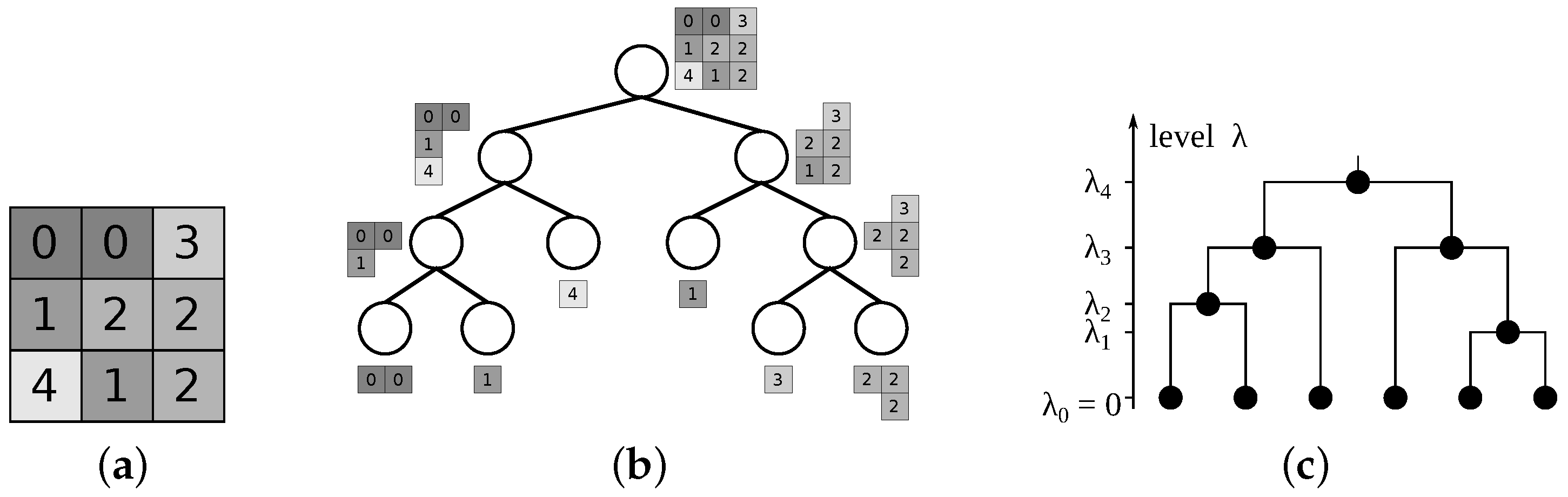
Figure 4.
A possible inclusion tree for the image displayed in (a) is shown in (b), with one possible dendrogram shown in (c). In this dendrogram, the gray nodes with represent new image elements entering the hierarchy, and do not belong to the support before then as indicated by the gray dotted line. The image extended by ghost pixels is shown in (d), with the links between original pixels shown in red and the links between the ghost and corresponding original pixels in violet. The extended tree shown in (e) is a partitioning tree for (d), with the auxiliary nodes (in green) identifiable as the singletons in the hierarchy.

Figure 5.
(a) The original image; (b) corresponding Min-tree; (c) the dendrogram; and (d,e) Max-tree and its dendrogram. Corresponding regions are shown next to the nodes.
Figure 5.
(a) The original image; (b) corresponding Min-tree; (c) the dendrogram; and (d,e) Max-tree and its dendrogram. Corresponding regions are shown next to the nodes.

Figure 6.
Upper and lower level sets of the image in Figure 5a (a,b); regions acquired by filling the holes of the level sets and forming the hierarchy (c); the Tree of Shapes (d); and the dendrogram (e).
Figure 6.
Upper and lower level sets of the image in Figure 5a (a,b); regions acquired by filling the holes of the level sets and forming the hierarchy (c); the Tree of Shapes (d); and the dendrogram (e).

Figure 7.
Creation of Binary Partition Tree on the flat zones of the original image in (a), using a constant gray level as the region model. The model is updated as the gray level of the larger of the child regions after a merge, or average in case of a tie. The merging criterion defines the dissimilarity as the difference between the region models. Merging order merges the region pair with the smallest dissimilarity first. Three merging steps are represented in (b–d). The constructed BPT is displayed in (e) and the numbers in the nodes indicate the merging order, with the indexed hierarchy dendrogram in (f).

Figure 8.
The original image (a); and partitions for α = 0 –3 (b)–(e), respectively, with edges between connected pixels shown in thin green lines and region borders in thick red; the α-tree (f); and the dendrogram (g).
Figure 8.
The original image (a); and partitions for α = 0 –3 (b)–(e), respectively, with edges between connected pixels shown in thin green lines and region borders in thick red; the α-tree (f); and the dendrogram (g).

Figure 9.
An example for the chaining effect for the image (a). The hierarchy of α-connected components has only two different levels (b,c). Although all pixel gray levels differ, the decomposition has no intermediate steps.
Figure 9.
An example for the chaining effect for the image (a). The hierarchy of α-connected components has only two different levels (b,c). Although all pixel gray levels differ, the decomposition has no intermediate steps.

Figure 10.
The partitions by levels of the (ω)-tree, for the original image from Figure 8a. Partitions for ω = 0–5 are shown in (a)–(e), respectively. The tree is displayed in (f), with the indexed tree displayed in (g).
Figure 10.
The partitions by levels of the (ω)-tree, for the original image from Figure 8a. Partitions for ω = 0–5 are shown in (a)–(e), respectively. The tree is displayed in (f), with the indexed tree displayed in (g).
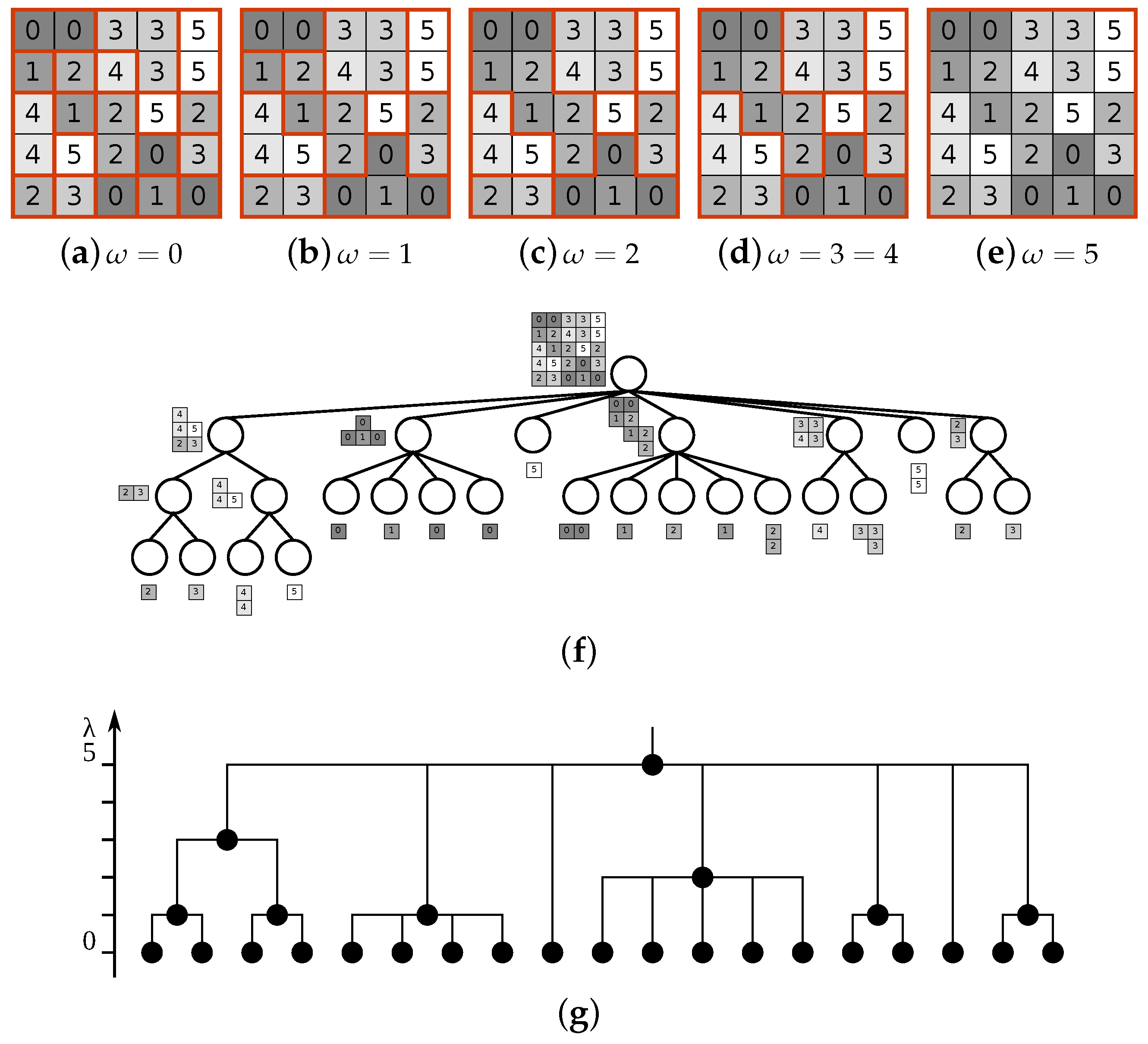
Figure 11.
Filtering the standard 256 × 256 grayscale Lena image using different trees. For all the trees except the BPT, the filtering was done by choosing a threshold level and keeping only the nodes above that level, using the library made by the authors1. The images for the BPT were generated by the tool presented in [109], which uses a different indexing method and filtering strategy. For every tree, a weaker and stronger filtering were performed, with the number of remaining nodes displayed in the sub-caption (except for BPT). Weak and strong filtering of the Min-tree (originally 15652 nodes) is shown in (a,b) respectively; and for the Max-tree (originally 15048) in (c,d). Filtering using the ToS (starting with 23796 nodes) correspond to: (e) weak; and (f) strong. The images resulting from BPT are shown: (g) weak filtering; and (h) strong filtering. The α-tree (76710 nodes) filtering results are displayed: (i) weak; and strong (j). Finally, filtering using the (ω)-tree (75185 nodes before filtering) is depicted: (k) weak; and (l) strong.


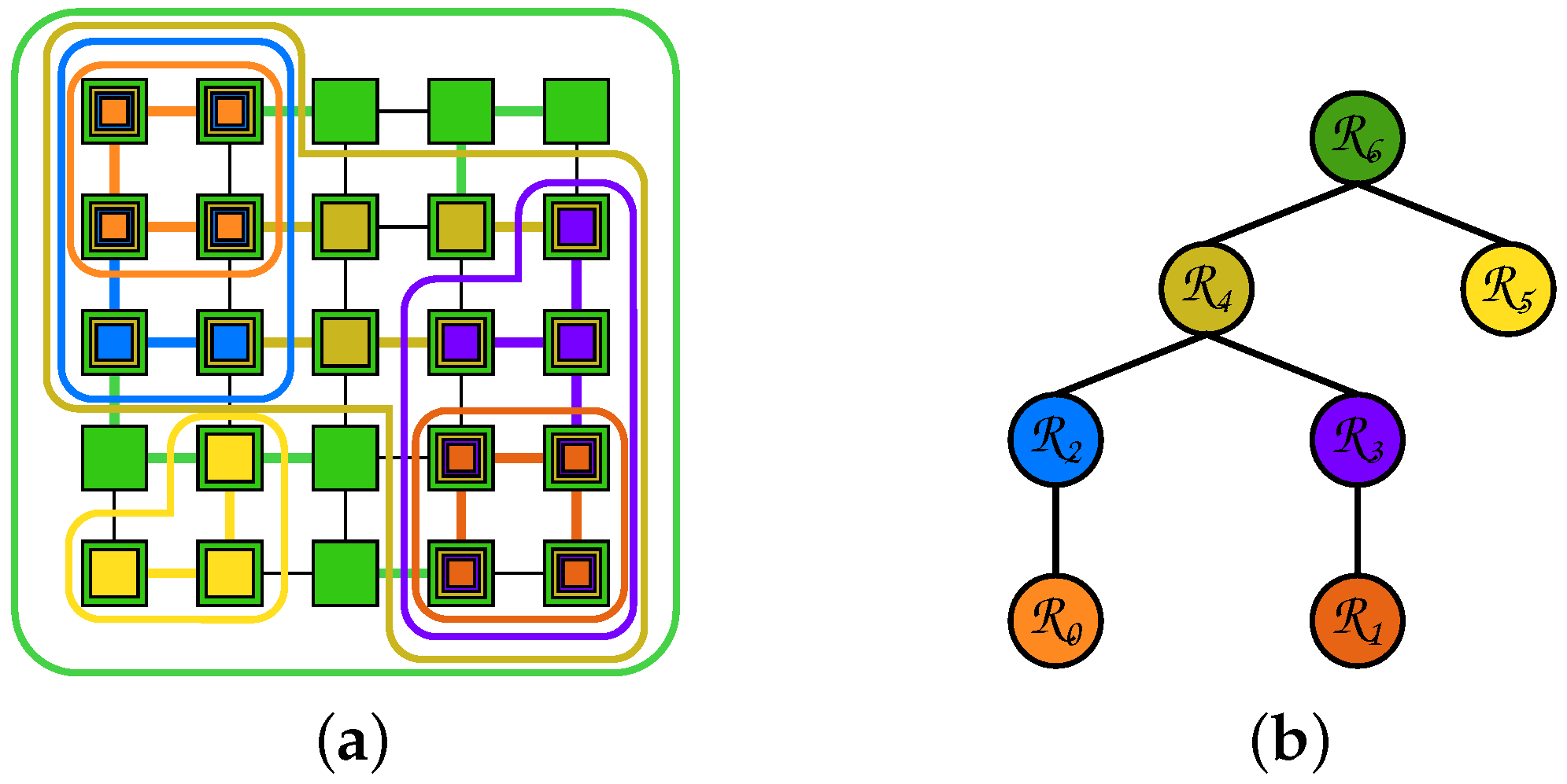
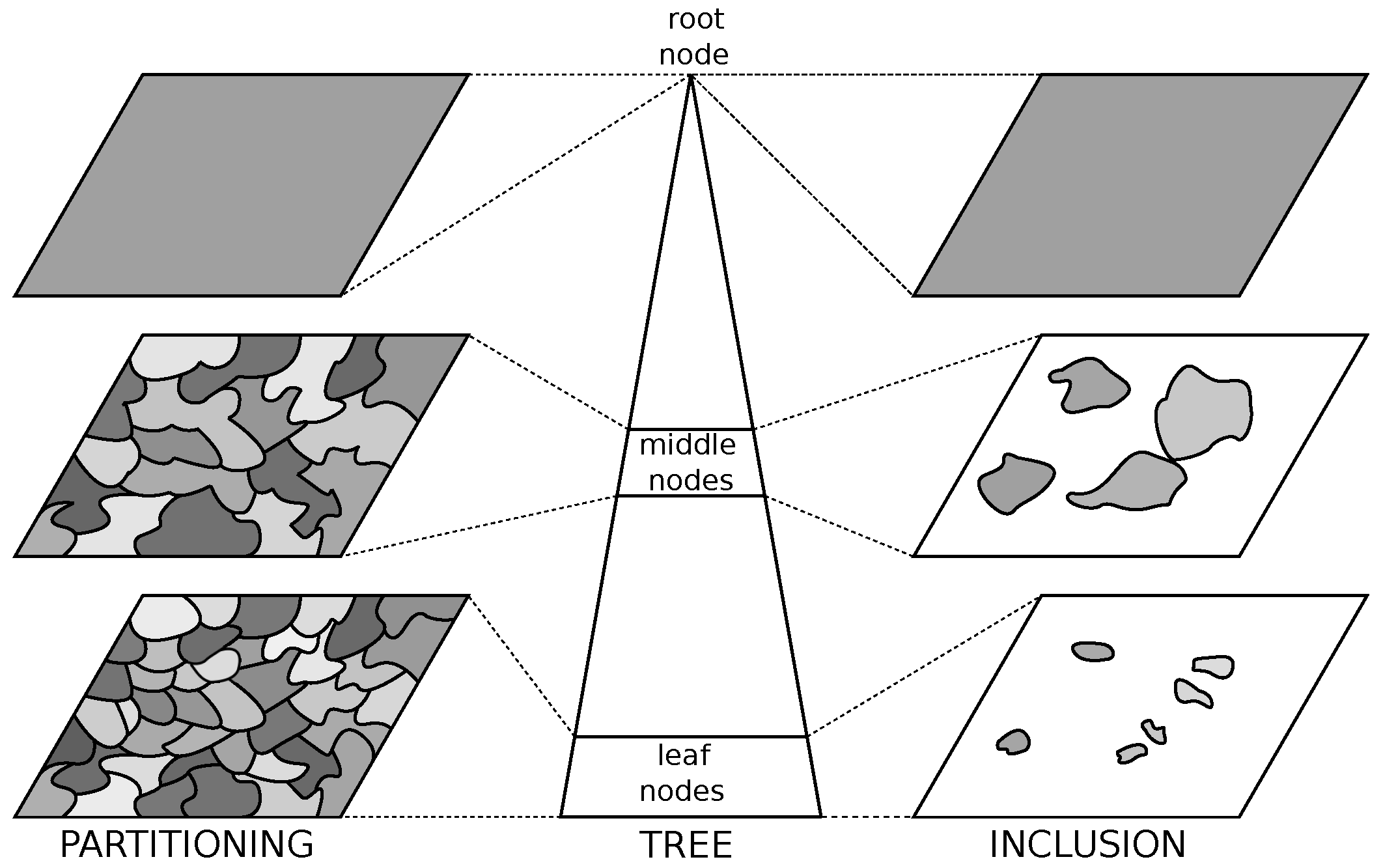
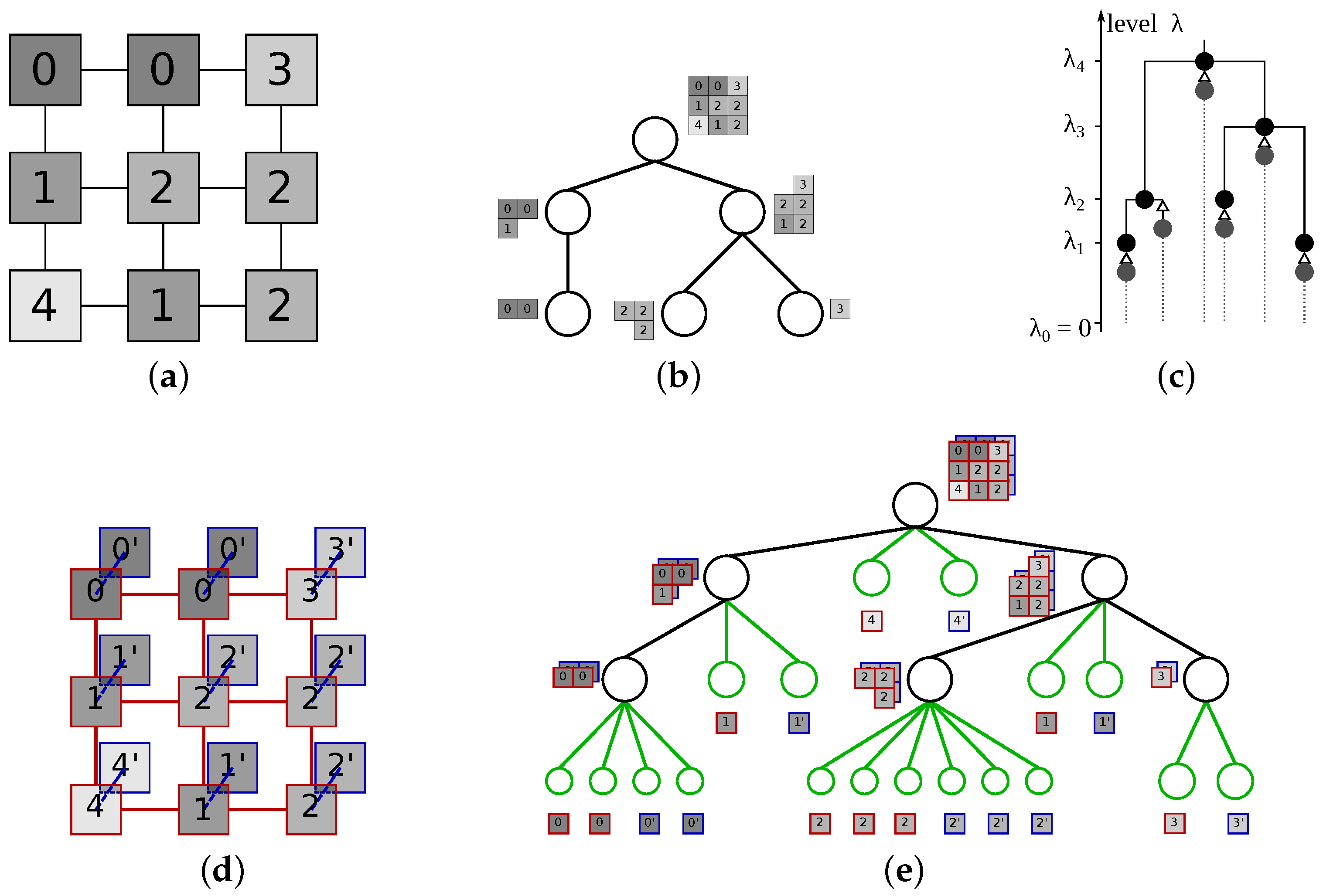
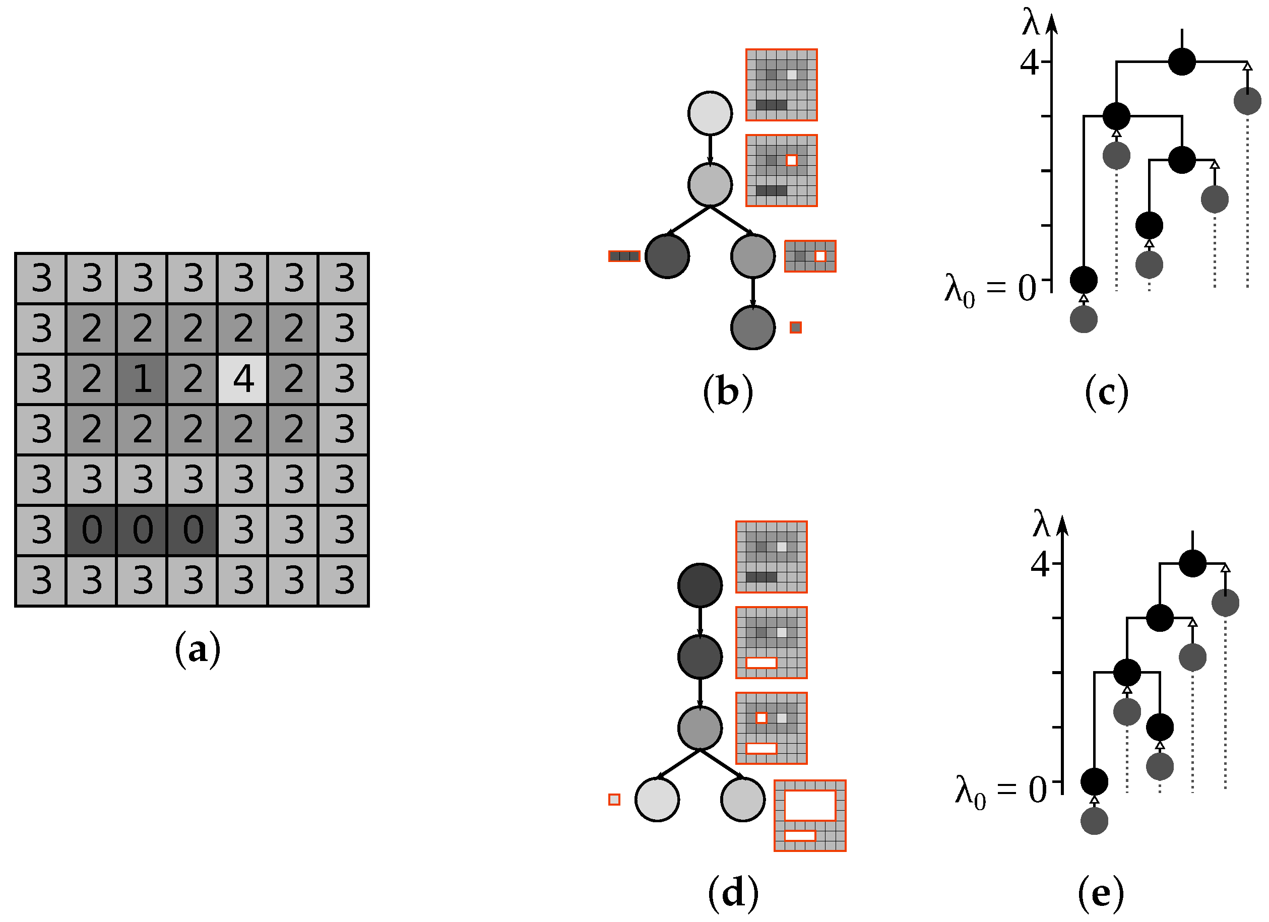
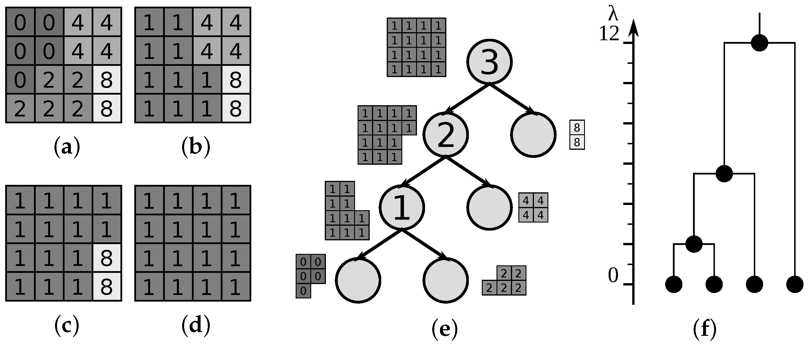
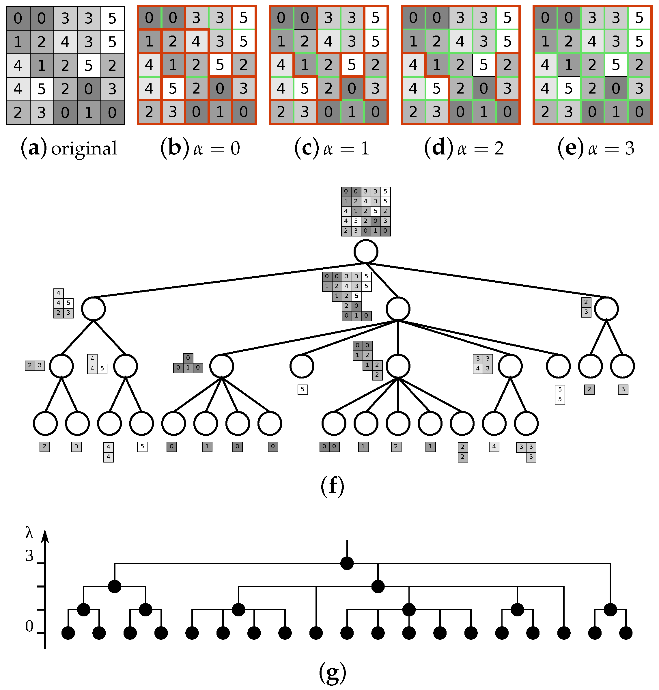
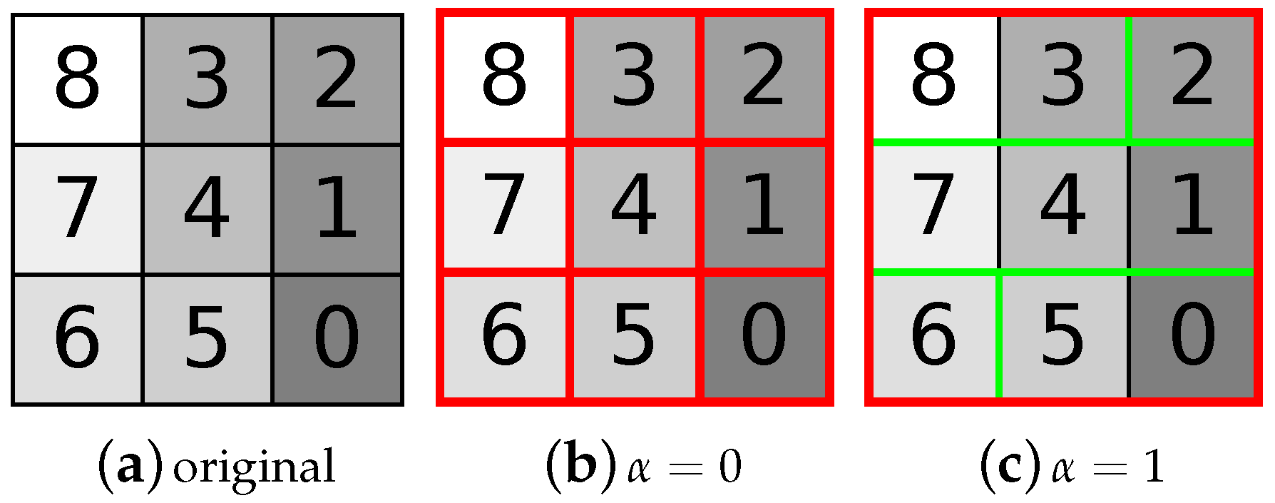
Table 1.
Summary of characteristics for inclusion trees.
| Tree | Max Tree | Min Tree | Tree of Shapes |
|---|---|---|---|
| Dual tree | Min tree | Max tree | self-dual |
| Type of objects | dark objects | bright objects | shapes |
| Complete representation? | Yes | Yes | Yes |
| Construction complexity | |||
| Additionalparameters | No | No | No |
Table 2.
Summary of characteristics for partitioning trees.
| Tree | Binary Partition Tree | -Tree | -Tree |
|---|---|---|---|
| Dual tree | self-dual | self-dual | self-dual |
| Type of objects | unions of initial partition | -CC (quasi flat zones) | -CC |
| Complete representation? | Yes | Yes | Yes |
| Construction complexity | |||
| Additional parameters | Initial partition, | No | No |
| region model, | |||
| similarity measure |
Depends on region model and similarity measure, but usually desirable. depends on the initial partition.
Table 3.
Some applications of the presented trees from the literature.
| Application Domain | Inclusion | Partitioning | |||
|---|---|---|---|---|---|
| Min/Max | ToS | BPT | -Tree | -Tree | |
| filtering/simplification | [28,52,85,105,113,114,115] | [37,65,116,117,118] | [52] | [42,95] | [42,119] |
| image/video segmentation | [28,29,114,120] | [117,118,121,122,123,124] | [2,109,125,126,127,128] | [42,44,129,130] | [42,44,119] |
| image compression | [131] | [124,132] | |||
| object detection & tracking | [133,134] | [25,135,136,137] | |||
| feature/edge detection | [103] | [83,138,139,140] | |||
| pixel/feature description | [62,141,142,143,144] | [63,144,145] | [146] | [146] | |
| image comparison | [37] | ||||
| change detection | [147] | ||||
| image retrieval | [103,142,148,149] | [140] | [150] | ||
| classification | [64,151,152] | [153,154,155] | [156] | ||
| time series processing | [157] | ||||
| astronomical imaging | [84,114,134,158] | ||||
| remote sensing (inc. hyperspectral imaging) | [62,64,141,143,144,147,149,152,159,160] | [63,144,145,155] | [126,127,128,135,136,161] | [153] | [119,156] |
© 2018 by the authors. Licensee MDPI, Basel, Switzerland. This article is an open access article distributed under the terms and conditions of the Creative Commons Attribution (CC BY) license (http://creativecommons.org/licenses/by/4.0/).
Share and Cite
MDPI and ACS Style
Bosilj, P.; Kijak, E.; Lefèvre, S. Partition and Inclusion Hierarchies of Images: A Comprehensive Survey. J. Imaging 2018, 4, 33. https://doi.org/10.3390/jimaging4020033
AMA Style
Bosilj P, Kijak E, Lefèvre S. Partition and Inclusion Hierarchies of Images: A Comprehensive Survey. Journal of Imaging. 2018; 4(2):33. https://doi.org/10.3390/jimaging4020033
Chicago/Turabian StyleBosilj, Petra, Ewa Kijak, and Sébastien Lefèvre. 2018. "Partition and Inclusion Hierarchies of Images: A Comprehensive Survey" Journal of Imaging 4, no. 2: 33. https://doi.org/10.3390/jimaging4020033
Note that from the first issue of 2016, this journal uses article numbers instead of page numbers. See further details here.