Article

Surface Mesh Reconstruction from Cardiac MRI Contours †

Institute of Biomedical Engineering, University of Oxford, Oxford OX3 7DQ, UK
*
Author to whom correspondence should be addressed.
This paper is an extended version of our paper published in: Villard B., Carapella V., Ariga R., Grau V., Zacur E. (2017) CardiacMesh Reconstruction from Sparse, Heterogeneous Contours. In: Valdés HernándezM., González-Castro V. (Eds.) Medical Image Understanding and Analysis. MIUA 2017. Communications in Computer and Information Science, Vol. 723. Springer, Cham.
J. Imaging 2018, 4(1), 16; https://doi.org/10.3390/jimaging4010016
Submission received: 8 November 2017 / Revised: 30 December 2017 / Accepted: 30 December 2017 / Published: 10 January 2018
(This article belongs to the Special Issue Selected Papers from “MIUA 2017”)

Abstract

:
We introduce a tool to build a surface mesh able to deal with sparse, heterogeneous, non-parallel, cross-sectional, non-coincidental contours and show its application to reconstruct surfaces of the heart. In recent years, much research has looked at creating personalised 3D anatomical models of the heart. These models usually incorporate a geometrical reconstruction of the anatomy in order to better understand cardiovascular functions as well as predict different cardiac processes. As MRIs are becoming the standard for cardiac medical imaging, we tested our methodology on cardiac MRI data from standard acquisitions. However, the ability to accurately reconstruct heart anatomy in three dimensions commonly comes with fundamental challenges—notably, the trade-off between data fitting and expected visual appearance. Most current techniques can either require contours from parallel slices or, if multiple slice orientations are used, require an exact match between these contours. In addition, some methods introduce a bias by the use of prior shape models or by trade-offs between the data matching terms and the smoothing terms. Our approach uses a composition of smooth approximations towards the maximization of the data fitting, ensuring a good matching to the input data as well as pleasant interpolation characteristics. To assess our method in the task of cardiac mesh generations, we evaluated its performance on synthetic data obtained from a cardiac statistical shape model as well as on real data. Using a statistical shape model, we simulated standard cardiac MRI acquisitions planes and contour data. We performed a multi-parameter evaluation study using plausible cardiac shapes generated from the model. We also show that long axes contours as well as the most extremal slices (basal and apical) contain the most amount of structural information, and thus should be taken into account when generating anatomically relevant geometrical cardiovascular surfaces. Our method is both used on epicardial and endocardial left ventricle surfaces as well as on the right ventricle.

1. Introduction

In recent years, much research has looked at creating personalised 3D anatomical models of the heart [1,2,3,4]. These models usually incorporate a geometrical reconstruction of the anatomy in order to understand better cardiovascular functions as well as predict different processes after a clinical event. Besides being fundamental to shape analysis, they are a prerequisite to electrophysiological and mechanical simulations with finite element analysis tools [5]. Furthermore, personalized shape models are increasingly used for surgical planing via 3D printing or device innovation [6,7]. However, the ability to accurately reconstruct heart anatomy from contoured magnetic resonance images (MRI) in three dimensions commonly comes with several challenges. The main challenge of standard cardiac magnetic resonance (CMR) is the slice misalignments in 3D caused by acquiring the images at separate breath holds. If corrected, the more notable challenge is the trade-off between data fitting and expected visual appearance of the resulting mesh. Most works in the literature tend to over regularize, or bias a data fitting process towards a smooth result [8,9]. Other methods work based on templates or shape prior, which are usually learned on normal patient anatomies, and tend to fail when presented with abnormal data, or any data outside the learned model [10]. Our approach differs in this, as we maximize the data fitting by composing smooth deformations on a smooth surface. In this paper, we propose a process to reconstruct a geometrical 3D surface mesh from a set of contours, partially representing an underlying heart shape anatomy, available from manual delineations or from automatic segmentations.
Whilst cardiac computer tomography (CT) images provide high anatomical resolution, contours obtained from CMR images were used as they provide additional information, non-invasively, about myocardial structure using techniques such as late Gadolinium enhancement or Diffusion Tensor MRI. In CMR, image acquisitions are typically composed of a stack of short axes (SAX) ranging from 8–12 slices, around 8 mm thick, with a 2 mm gap between slices, and one or more long axes (LAX). Contouring (also know as segmentation or delineation of the anatomical structures) of these typical acquisition protocols result in a spatial configuration of curves delimiting the anatomical structure of interest. These sets of curves are sparse since usually within the SAX stack they are 10 mm apart leaving large gaps to be filled, and cross-sectional since they comprise SAX as well as LAX view contours. Manual or automatic contouring methods are seldom able to account for the 3D environment, which can lead to spatial inconsistencies between long axes and short axes’ contours. Due to the delineations not being able to grasp perfectly the global 3D shape of the heart, contour-to-contour distances between these contours cannot be minimized to obtain perfect coincidence and therefore spatial 3D consistency [11].
A good example of this occurs in LAX, where papillary muscles can be hard to differentiate from myocardium, which can result in their inclusion in the myocardial volume, in spite of their exclusion in SAX. Furthermore, due to the image acquisition occurring at different breath holds, as well as any patient movement inside the scanner, the contours might be misaligned. This tends to further increase their discrepancies and extra steps might be needed to correct for this misalignment [11]. This post-acquisition correction of the pose of the images can lead to losing the parallelism in the SAX stack. Finally, since many cardiomyopathies are localized in the left ventricle (LV), many previous efforts were focused on methodologies specifically designed or tuned for the LV. This paper is an extension of our conference paper [12]. There exist significant extensions—notably a thorough evaluation of the reconstrucion parameters, as well as the use of a statistical shape model to generate realistic anatomical shapes allowing a broader and more comprehensive assessment of our technique.
The main contributions of this work are:
  • Development of a surface reconstruction method capable of dealing with non-parallel, cross-sectional, sparse, heterogeneous, and non-coincidental contours,
  • Use of our technique on the surfaces of the left ventricle as well as on the right ventricle,
  • Evaluation of our method on several realistic shapes generated from a statistical shape model, as well as on real data data consisting of normal and abnormal pathologies.

State of the Art

Whilst simple heart models can be used for electrophysiological or mechanical studies, patient-specific meshes require more complex and accurate anatomical models [13]. These models are commonly characterized through 3D meshes, on which shape analysis or finite element methods can be performed. From a set of contours, or eventually, point cloud, a surface mesh can be generated and act as an input to create a volumetric mesh. Depending on the complexity of the surface mesh needed, many parameters need to be taken into account—notably the trade-off between data matching and expected visual appearance of the resulting mesh [2,13]. The prior art for mesh reconstruction is considerable, and we invite the reader to consult [14,15,16] for a more in-depth look into current techniques.
Many approaches have been developed in order to produce surface reconstructions from planar contours; however, we were unable to find any method to work with our data consistently, or with data formed by parallel or quasi-parallel noisy contours, with or without cross-sectional information, that may or may not be coincidental. Furthermore, as CMR data is quite sparse, since each of the SAX contours lie around 10 mm apart, we needed a method that worked robustly on non-dense datasets.
According to [16,17], surface reconstruction methods broadly fall under three distinct categories: region growing, computational geometry, and functional methods, all of which can be further divided into interpolating or approximating methods.
Region growing algorithms propagate information from all the points, starting from an initial seed. The most notable of these methods is the ball pivoting algorithm (BPA) [18]. The ball pivoting algorithm is an interpolating technique to generate an alpha-shape surface given an oriented point cloud. In 2D, given an initial seed point, a circle of a chosen radius iterates from point to point connecting them via edges. This process can be extrapolated to higher dimensions. This technique can tend to fail for complex geometries and as they rely on point normals they are more suited for dense point clouds, with well defined normals.
Computational geometry methods explore all the surrounding neighbourhoods of all the sample points in order to find the best neighbouring candidate points for each of the samples. The most prominent of these techniques is the Delaunay triangulation. Delaunay triangulation is an explicit method that relies on finding a unique triangulation for all points given a set of points [16]. Lim et al. [19] use Delaunay triangulations in order to reconstruct a cardiac mesh given a set of parallel SAX contours. By computing a connectivity tree between the set of contours, they project adjacent contours onto a 2D plane, where a Delaunay triangulation is computed between the contours, before projecting them back to 3D. Another technique when presented with sparse planar point clouds is to interpolate between the planes. Many algorithms exist to interpolate between contours; however, results are not reproducible between algorithms, which causes discrepancies in further analysis [3]. The method in [20] starts with an initial mesh and proceeds to iteratively refine the mesh. However, equivalently to [2], the input data must have coincidental points at the intersection for the method to work.
Functional methods tend to find a function that best approximates a surface given a set of points, via sets of functions. In [2], the surface mesh is constructed by optimising over the topology, using a level-sets approach, and having the genus as a control parameter. In order for the resulting mesh to represent the most accurate anatomical representation, an image volume is necessary. One of the drawbacks of the method is for the contours needing to have coincidental points at their intersections, which prevents the method from being used on standard CMR acquired data. To obtain uniformly distributed contour points, the authors in [21,22] first fit a cubic periodic B-spline curve to the contours, allowing them to uniformly sample candidate points. The disadvantages of this approach is that it relies on the the number of control points selected, which in turn, smooths the overall mesh. The use of a template mesh in [9] can also cause the resulting mesh to be biased to the template. When presented with abnormal data, this bias will cause the resulting mesh to be unable to retrieve the abnormal shape. In the Poisson surface reconstruction technique [23], an implicit function is fitted to the data using provided point normals, after which the reconstructed surface is obtained by extracting an isosurface. Similarly to the BPA algorithm, this method can tend to fail for complex geometries. Our method differentiates itself from these other works as it only utilises the input data without the need for normal calculations or for the contours to be coincidental.

2. Materials and Methods

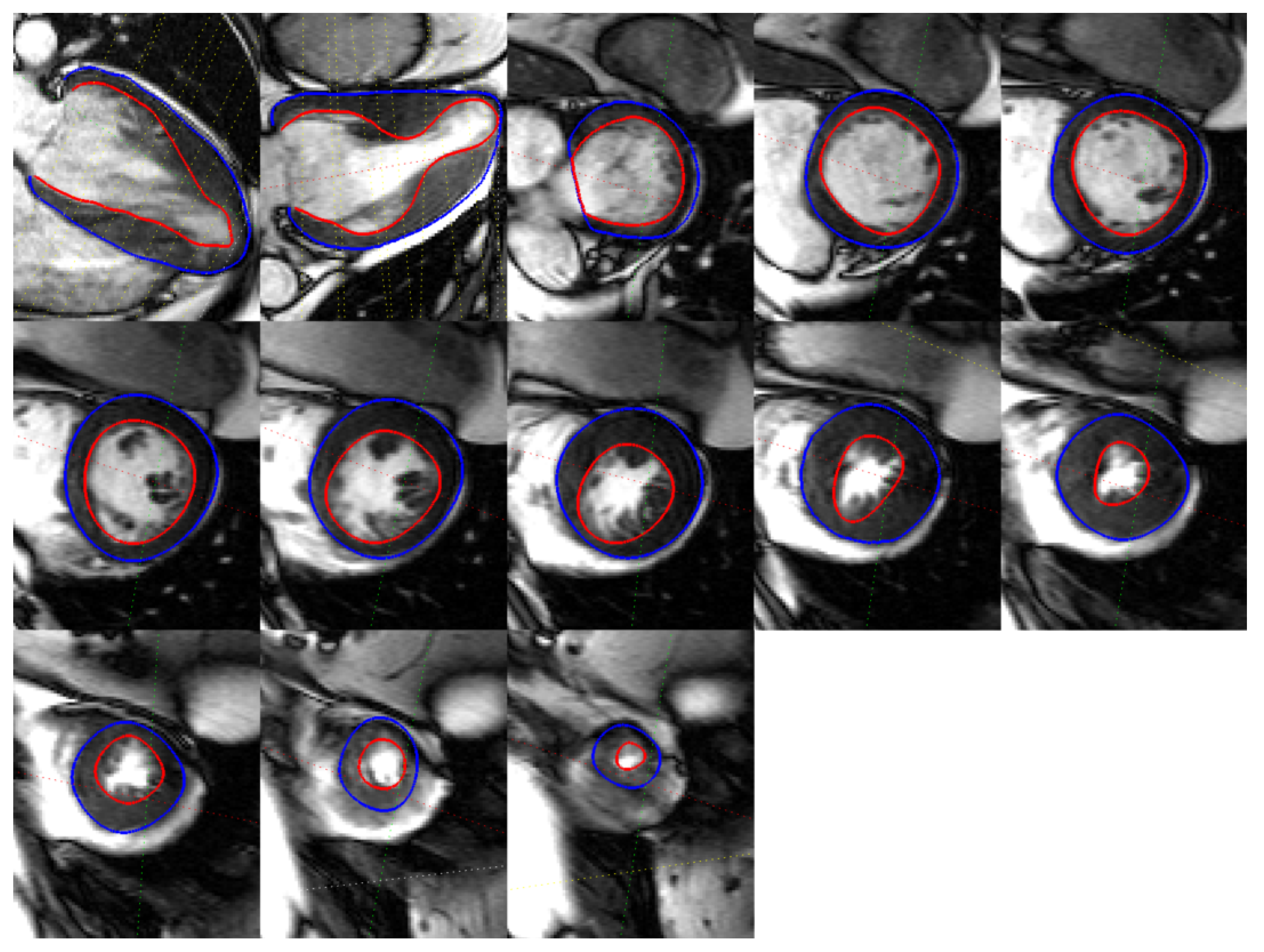
2.1. Synthetic and Real Data
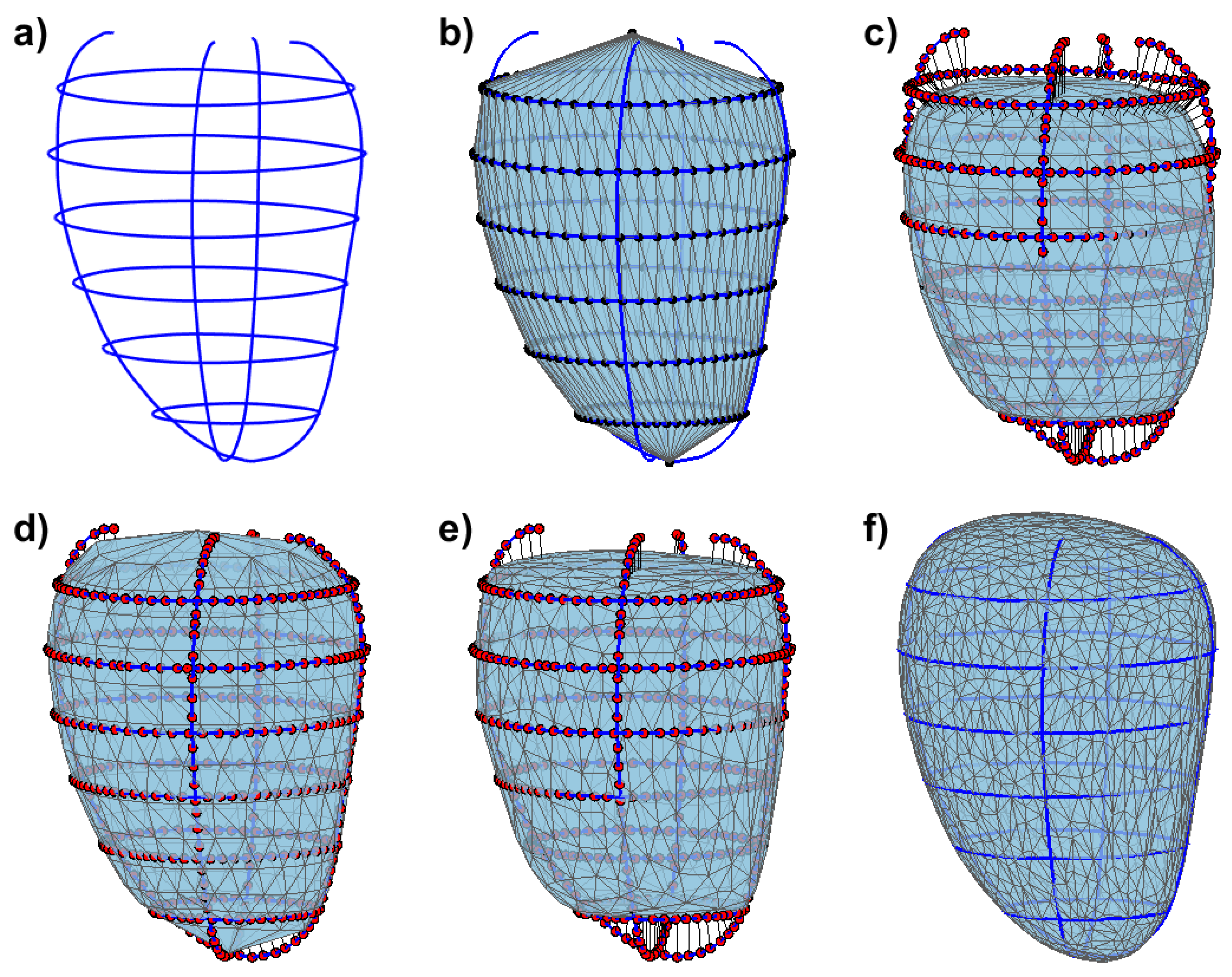
Both synthetic and real datasets were used. Synthetic data were generated through the use of a statistical shape model (SSM) obtained from [24,25] and is available online (http://wp.doc.ic.ac.uk/wbai/data/). Using the modes of variation, different plausible heart-like shapes were generated and used in our experiments. Having the SSM allowed for a quantitative evaluations of our method, since the generated meshes provide ground truth anatomies. Contours were synthesized by slicing the generated meshes at various spatial positions. Parallel and non-parallel contours, simulating a short axis stack, and cross sectional contours, simulating LAX, were produced and used as inputs to our method. We treated the generated shape meshes as ground-truth and compared our results against it. Regarding real data, we synthesised data by fitting the shape model to real contour data by optimizing the contour-to-mesh distances between the shape model and the contours.
The SSM was fitted to the segmented contours, applying Equation (1). In doing so, we obtained the set of parameters b and transformation T that allowed us to generate the closest possible shape matching the provided contours. As the SSM was acquired from non-abnormal geometries, we used non-abnormal data as the SSM would not be able to generate abnormal shapes if fitted to irregular data. In order to fit the SSM to the data, we minimized the contour-to-mesh distances, such that:
min b , T k i d ( C k i , T ( X ¯ + Φ b ) ) 2 ,
where C k i is the i-th point on the k-th contour, X ¯ the mean shape model, Φ = ( ϕ 1 , ϕ 2 , ) are the SSM modes of variations, b are a set of parameters that, when applied to Φ along with the rigid transformation model T , generate a new shape. The error metric d is the contour-to-mesh distance. For each of the contours, the shape model with the minimum contour-to-mesh distance was obtained, and a set of spatially consistent contours were generated by slicing the mesh at the same planes as the CMR acquired contour planes. Figure 1 shows an example of such a mesh.
In such a manner, we used 40 normal subjects to synthesize different meshes. These meshes were sliced at the same planes of the real contours, thus generating spatially consistent simulated contours, having the same spatial planes as standard CMR acquisitions. This allowed us to have a ground truth mesh with no spatial inconsistencies. Delineated normal and abnormal contours, acquired from cine images at end-diastole were used, which were obtained from a collection of CMR cases from the John Radcliffe Hospital, Oxford, UK (UK ethical approval IRAS project ID: 112814). We define normal and abnormal following the anatomical appearance and clinical condition of the subject. In order to not bias our quantitative assessments, we selected cases that had the same amount of slices, as this is roughly indicative of the hearts having the same height, since the images are taken at regular intervals. Finally, our data consisted of 24 cases, 10 normals, and 14 abnormals randomly selected from the previously mentioned collection. All of the cases were chosen as they have 11 contours, two LAX and nine SAX.

2.2. Initial Meshes

Our method requires an initial mesh M 0 . This mesh can be computed using various approaches, such as the convex hull of the input data, or by fitting a precomputed mesh to the data such as the meshes found in [8,9,19]. In our case, M 0 is computed as a tubular mesh connecting the contours, as explained below. Let C j be a set of contours, each lying on a plane with normal n j , where j is the contour index. A central direction is computed among all normal directions by computing the myriad following [26]. All normals lying within a neighbourhood of 20 degrees from that central direction are clustered together and their mean direction is used as main direction representing the long axis. In addition, the contours with normals in belonging to that cluster (which are expected to be the ones in SAX view) are then sorted from the most apical to the most basal (see Figure 2a). Two extra points are added to C j providing an upper and lower lid, to fully enclose the initial mesh. We then proceed to create a rough initialization of the mesh by constructing a tubular surface going through the contours. For each of the contours, distribute K equally spaced contour points. A ruled surface approach is then used to obtain an initial mesh, where the initial triangle making up the mesh are composed of the set ( C j ( i ) , C j ( i + 1 ) , C j + 1 ( i ) ) , ( C j + 1 ( i ) , C j + 1 ( i + 1 ) , C j ( i + 1 ) ) , with i being the point index of the contours after resampling (see Figure 2b). Depending on the availability of the LAX information, the algorithm initializes the lower bound mesh point from the lowest contour points in that plane, representing the apex, by using the LAX information. Analogously, the same can be done in the upper part of the mesh, where the upper mesh point, representing the most basal slice, is initialized as the mean position of the topmost contour points lying on the plane that contains such point.

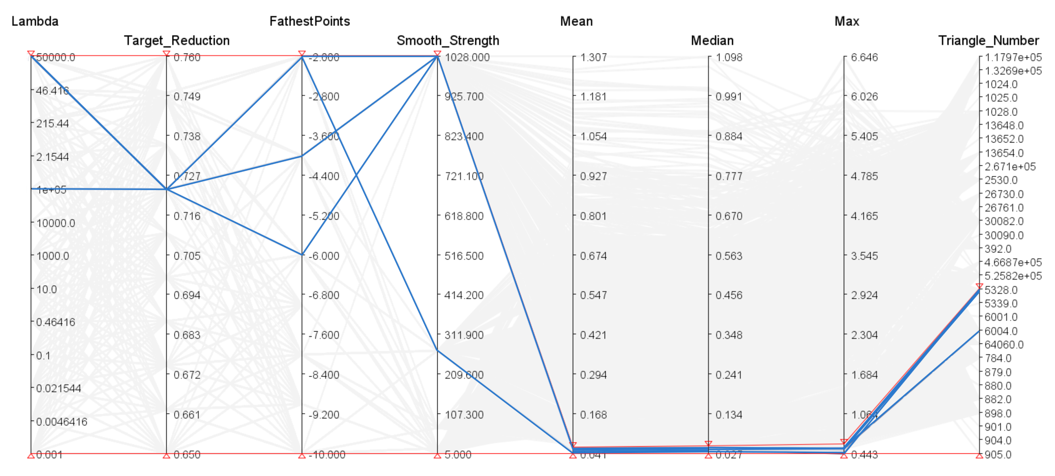
2.3. Mesh Deformation
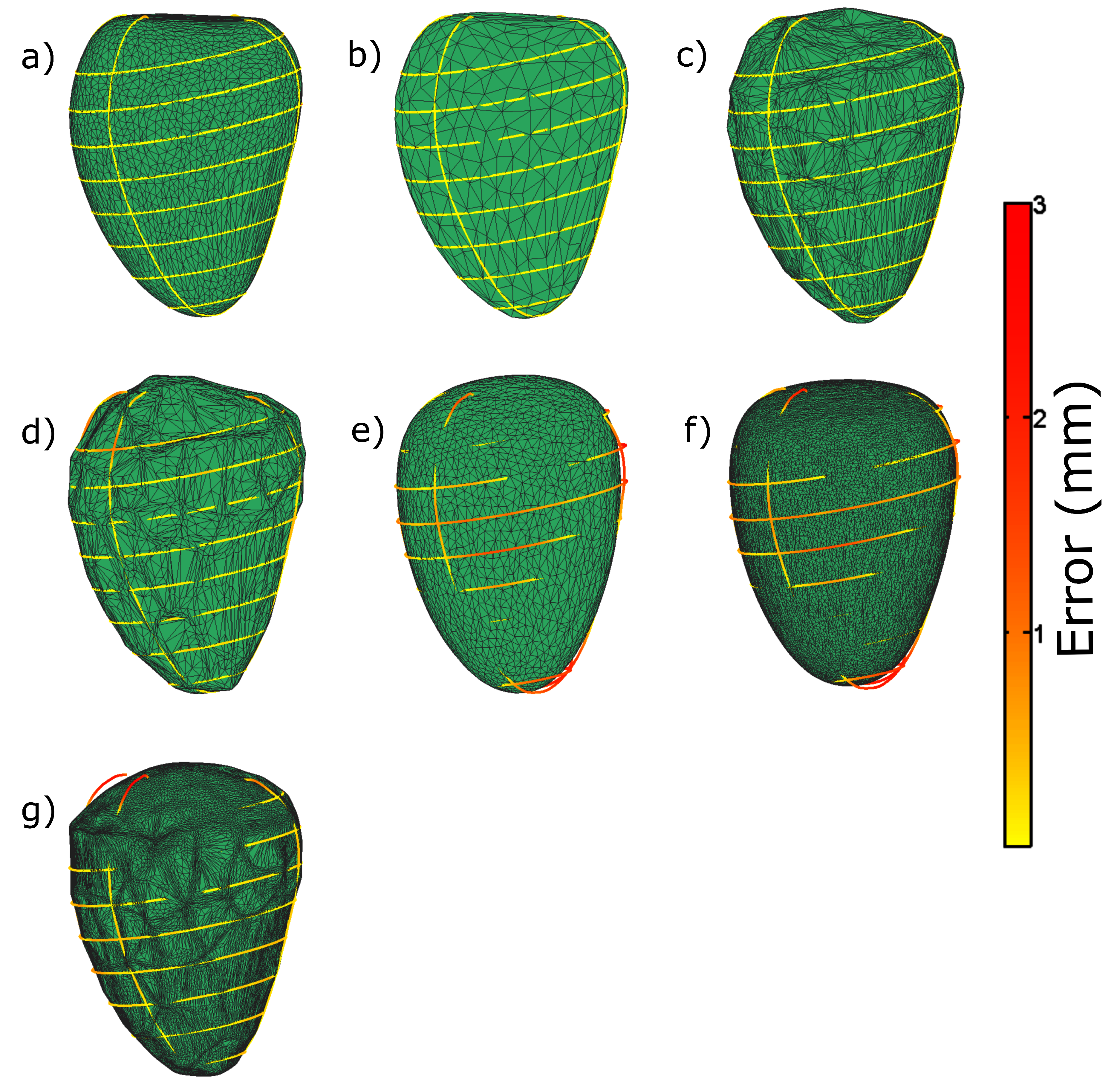
As the initial selected points make up the mesh, another set of contour points are selected as the data fitting terms, and act as attractors for the mesh. N points are sampled, using farthest point sampling, allowing for a representation of the global spatial distribution of the contour points. The farthest point sampling method [27] ensures that no contour is sampled more densely than any others. At this point, the initial mesh M 0 , the contours, and the attractor points are all scaled to a common reference frame that is irrespective of the units of the provided contours. Once all the preprocessing is achieved, a deformation field is computed by taking the closest point from each of the attractor points on the contours to M 0 . The points on M are pulled towards the corresponding attractor points, and this deformation is extrapolated via the use of approximating thin plate splines (TPS) [28,29]. We apply this process iteratively in small consecutive steps, to ensure small, smooth deformations as per Equation (3). Let P i , lying on the surface M t , be the set of closest points to the attractor points Q i . Let F : R 3 R 3 be the deformation field such as
argmin F λ i = 1 ( F ( P i ) ( Q i ) ) 2 + J m d ( F ) ,
with
Q i = P i + β ( Q i ) ( P i ) ( Q i P i ) ( Q i ) ( P i ) ,
where J m d is the TPS functional using derivatives of order m, and d the image dimensions, as defined in [28,29]. In our case, we use J 2 3 . It should be noted that λ affects the data matching term. With the computed F, we perform a deformation M t + 1 = F ( M t ) iteratively, in a diffeomorphic manner, resulting in a composition of several smooth approximations approaching M towards the contours. This is is seen in Equation (3), where Q i is the location of the deformation applied on points P , towards Q as a factor of β . It can be shown that the points P asymptotically converge to Q . Once the mesh has been deformed, the mesh undergoes subdivision to increase its resolution, allowing for a more appropriate reconstruction of the geometry. We use the interpolating butterfly subdivision algorithm [30], allowing us to increase the number of vertices, in a rounded manner, whilst keeping the position of the original vertices. Afterwards, we smooth our mesh using Laplacian smoothing, which can be seen in Equation (4) [31], allowing us to clean and fair our mesh. The Laplacian smoothing is performed in the following manner:
L ( p i ) = 1 j N i j N i p j p i ,
where p represents the vertices, and p j represents the adjacent vertex to p i . It is well known that this smoothing operation usually shrinks the mesh [32], and as such we follow the smoothing with an affine transformation between the original and final positions of the vertices. As the subdivision process can lead to extremely high amounts of triangles, the mesh is decimated, using quadratic decimation, which allows for some control over the amount of triangles while preserving its geometric characteristics [33].
The latter steps of subdivision, smoothing, and decimation occurs every S iterations. The overall pipeline can be seen in Figure 2. The overall process starting from the farthest point sampling is repeated for a set number of iterations, or until some stopping criterion is achieved, such as the contours-to-mesh distance falls bellow a chosen threshold or a fixed number of iterations has been reached. In our case, we empirically found that good quality meshes were found after 250 iterations. That stopping criterion was used along all experiments performed in this work.

3. Results

In order to assess our algorithm, we performed a series of experiments on both synthetic and real data, allowing us to assess all the different aspects of our methodology in a pertinent manner.

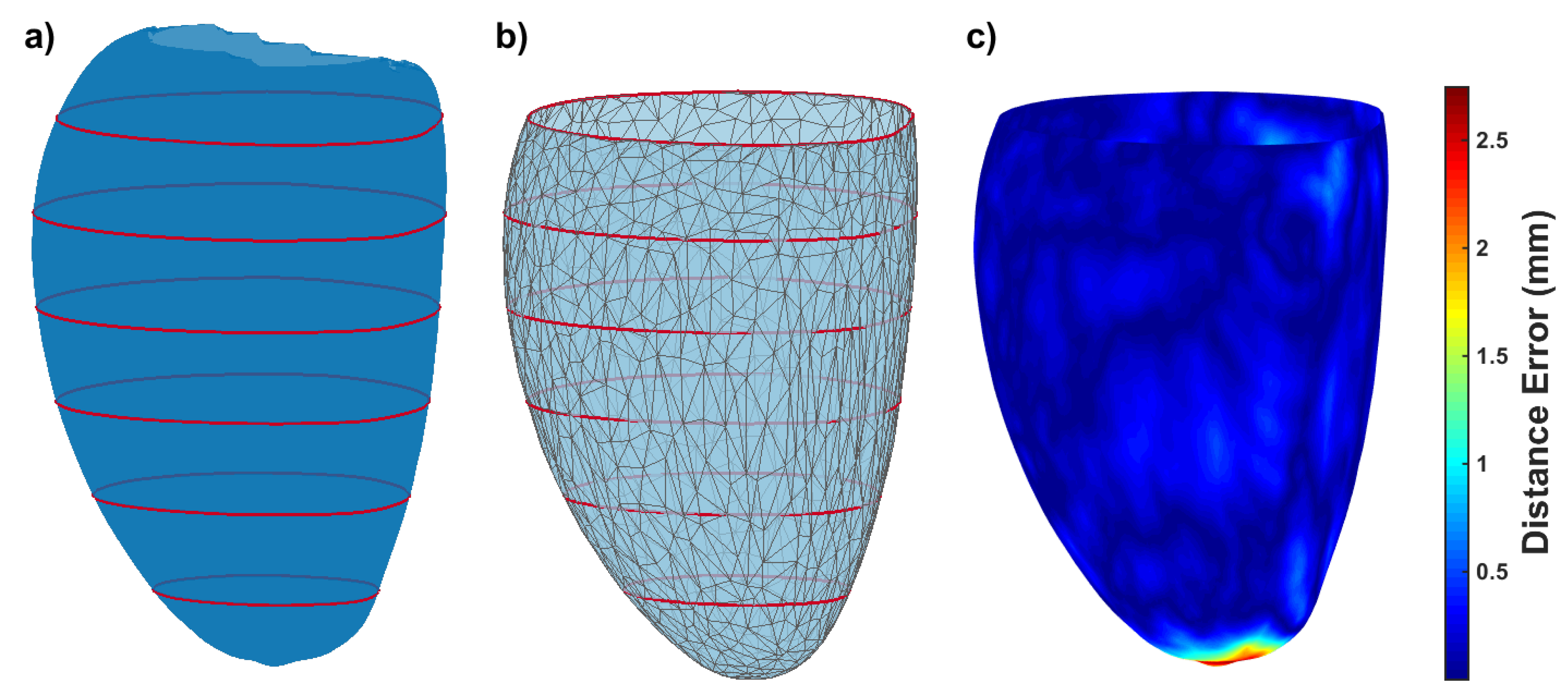
3.1. Simulation of CMR Acquisitions
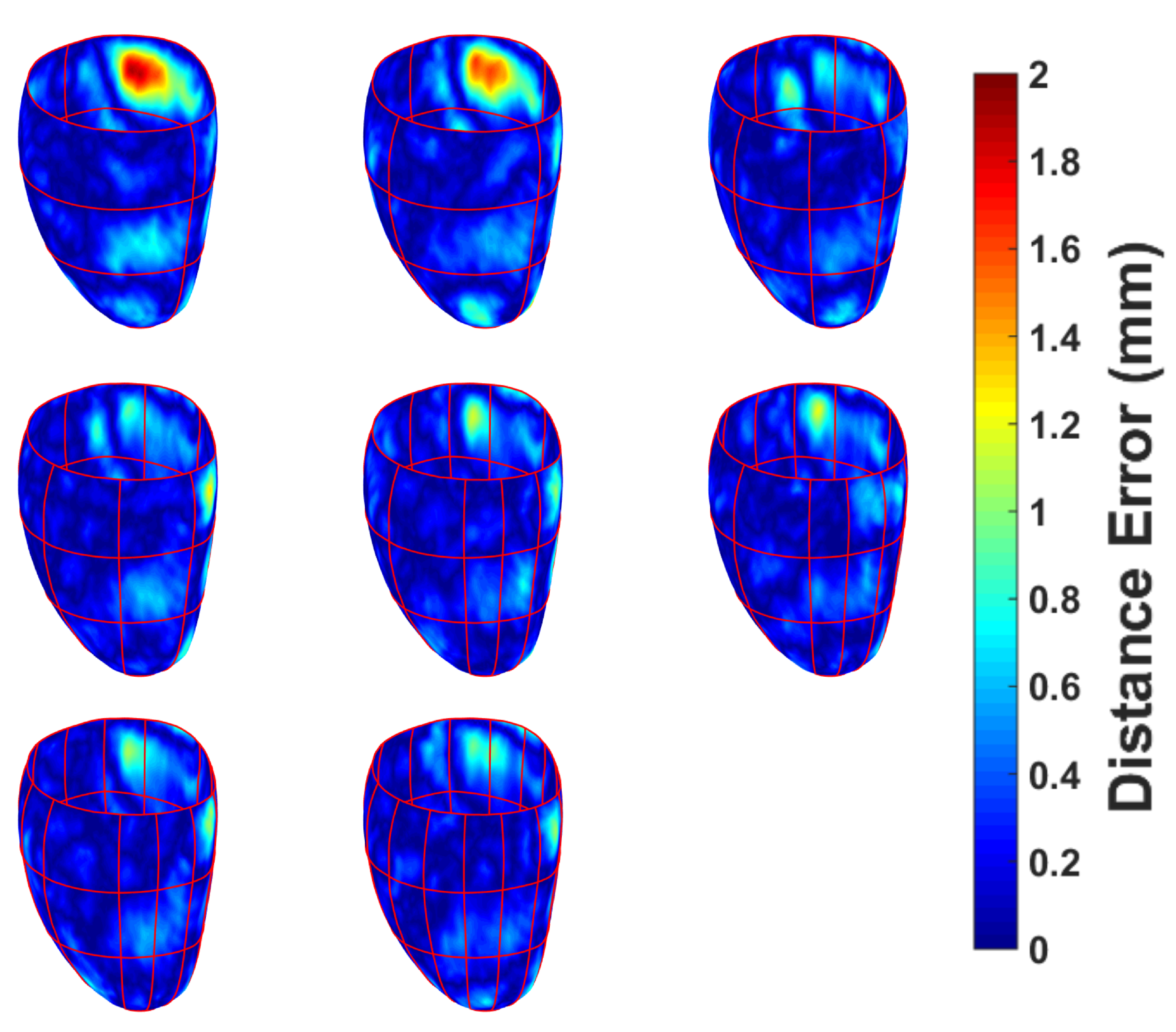
Our mesh construction methodology requires a number of parameters to be chosen. Some parameters, such as the TPS regularization term λ or the number of Laplacian smoothing iterations, have an explicit effect on the overall resulting shape, whilst for others such as the farthest points sample size or the decimation parameter, this effect is less obvious. In order to evaluate good candidate parameters, we performed a multi-parameter study using synthesized contours from several instances of the SSM fitted to real contours.
A parallel coordinate plot, as shown in Figure 3, allowed us to select the default parameters to generate our meshes. Each parameter has a certain effect on the resulting surface mesh. It can be seen in Equation (2) that the λ parameter controls the data matching strength. The higher λ is, the more reliant on the contours the method will be. In contrast, the lower the λ , the more spherical the resulting mesh will be. It can be noted, from the parameter exploration, that the Laplacian smoothing term, which is represented by the amount of iterations of L , and λ are linked with respect to data matching. Even with the lowest λ possible, if there is a low number of smoothing iterations, the resulting mesh will be close to the contours, but will be subject to the amount of decimations. As such, the mesh will tend to be quantitatively close to the contours but appear very wrinkled. It should be noted that, with a high number of decimations, the number of triangles increases, and can act as curvature control term. The higher the amount of decimations, the more curvature is possible, with regards to the overall mesh. Whilst this can result in a smoother looking mesh, the mesh has the possibility to be very convoluted. The farthest points parameter, controlled by the minimum inter-points distance allowable, does not appear to have much of an effect on the overall smoothness of the mesh, or the contour matching. However, as most of the normal case meshes, especially for the epicardium, can be geometrically simple (resembling a cylinder), the number of points needed to describe the geometry is low. With more convoluted geometries such as with some of the more severe abnormal cases, the lower the farthest points distance, the more likely the overall geometry will be captured. Figure A1, in Appendix A, shows several cases for extreme parameter values.
In our case, the best parameter sets were found with a very high λ , a target reduction of 72.3 % , and a small farthest point distance (from 2 to 4 mm inter-point distance). The red bands in Figure 3 show the cut off values for the parameters selection. Our method was initially tested in several scenarios and extreme values for its parameters were found empirically. Once extremal parameter values were found, each parameter was sampled accordingly. Some parameters, such as the target reduction, were sampled linearly, whilst others, such as λ , were sampled logarithmically. Using the cut off values on our requirements resulted in the most visually pleasing meshes with low mesh-to-mesh errors. These parameters were used for all of the resulting meshes in all of the experiments.
Table 1 represents the mean, median, min and maximum mesh-to-mesh distances for the epicardium, endocardium, and right ventricular for 40 cases, having used the simulated contours described in Section 2.1 as inputs. This experiment allowed us to simulate contours at the same spatial poses as CMR acquired images. Furthermore, having fitted an SSM to real data, allowed us to obtain various shape models based on patient population. This allows us to assess the robustness of our methodology to the variations of shapes seen in the population. By having a ground truth mesh, we were able to compare our results in a quantitative manner without the inherent contour discrepancies. The resulting meshes, showing the different shape variations, can be seen in Figure A2, Appendix B.

3.2. Synthetic Data

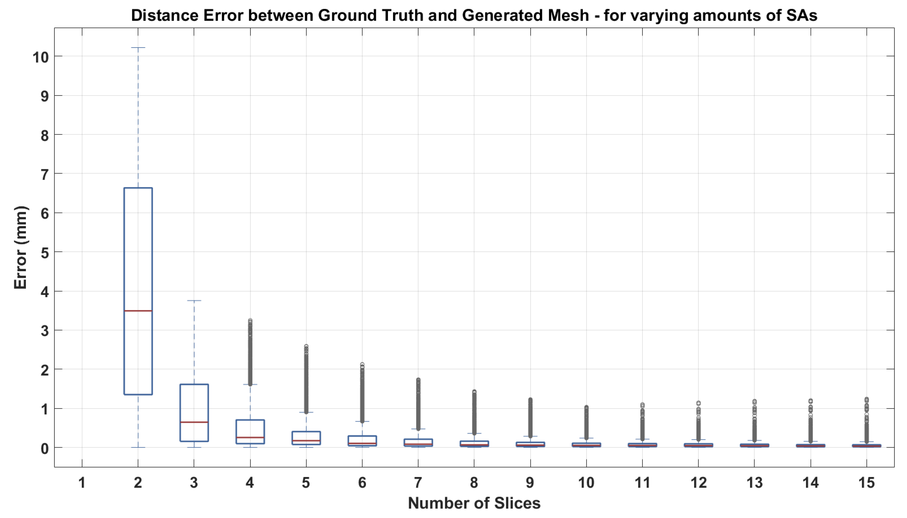
3.2.1. Short Axis Contours

In a first instance, we applied our method to a set of parallel SAX contours and observed the ability of our technique to recover the ground truth mesh by evaluating the mesh-to-mesh distance error. Our validation consisted of calculating the distances between vertices of our generated mesh to the ground truth mesh (mean shape of the statistical model) as shown in Figure 4. We also assessed the effect the number of SAX had on the ability of the mesh to recover the original mesh by increasing the amount of SAX contours provided initially from 2 to 15, between the base and the apex. The results can be seen in Figure 5.

3.2.2. Short Axis and Long Axis Contours

In a second experiment, we assessed the impact providing LAX contour information had. Similarly to the first experiment, we looked at varying the amount of LAX contours and the effect it had on the overall mesh result, as well as look at the influence LAX positions had. Four SAX contours were chosen, and an increasing amount of LAX contours were provided as the initial input by adding a rotated version of the initial LAX contour every iteration. From an initial LAX, rotated versions were iteratively added using the following rotations: 90, 45, 135, 22.5, 157.5, 112.5, 67.5 degrees, respectively. Similarly to Section 3.2.1, the same analysis was performed. The mesh-to-mesh contour distance was calculated and overlaid on the ground truth mesh, as shown in Figure 6.

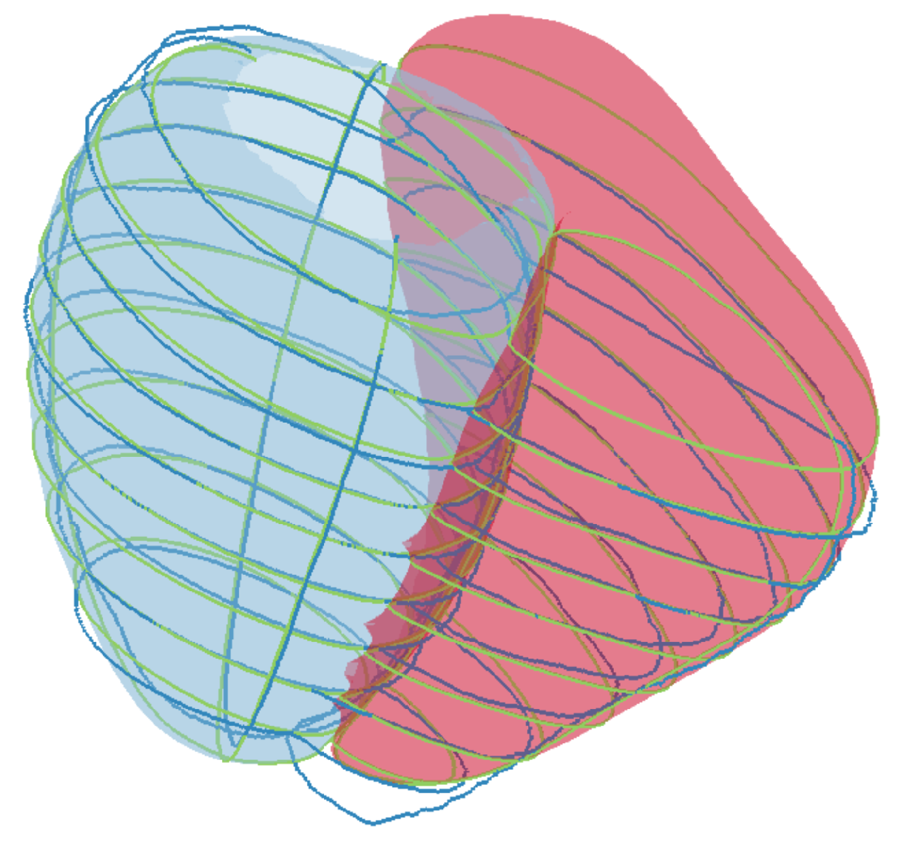
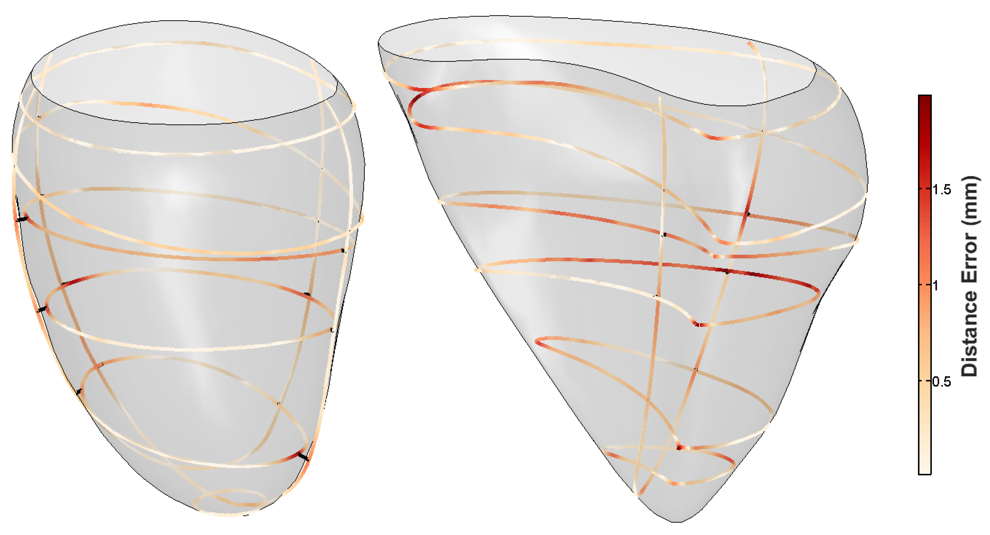
3.2.3. Non-Parallel, Non-Coincidental Contours

As our method is intended to be used with real data, we mimicked a standard acquisition. From the mean shape model, 10 SAX contours (resulting in 10 mm inter-slice distance) as well as two LAX contours (simulating two and four chambers’ views) were generated. The contours were then perturbed, mimicking breath-hold related misalignment, by applying small random translations and rotations (in plane as well as out of plane). The translation and rotation perturbations were performed within the ranges described in [34,35]. The resulting non-parallel, non-coincidental contours were given as an input to our algorithm. The resulting mesh can be seen in Figure 7a. The distance map overlaid on the contours is the distance from the resulting mesh to the input contours. The algorithm was also tested on a right ventricle, as seen in Figure 7b.

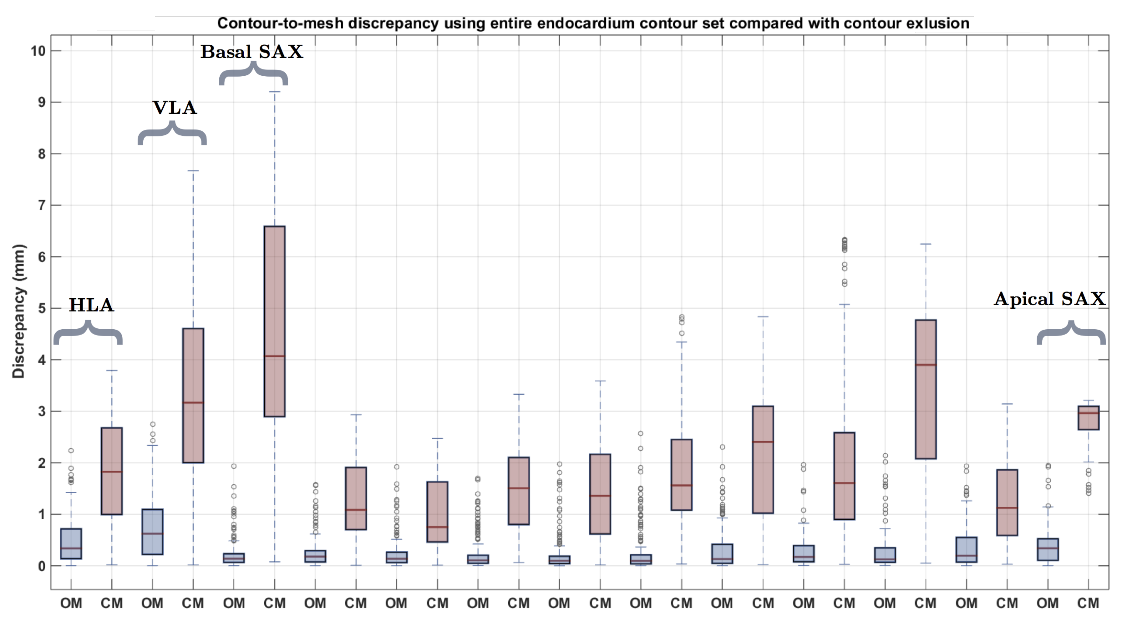
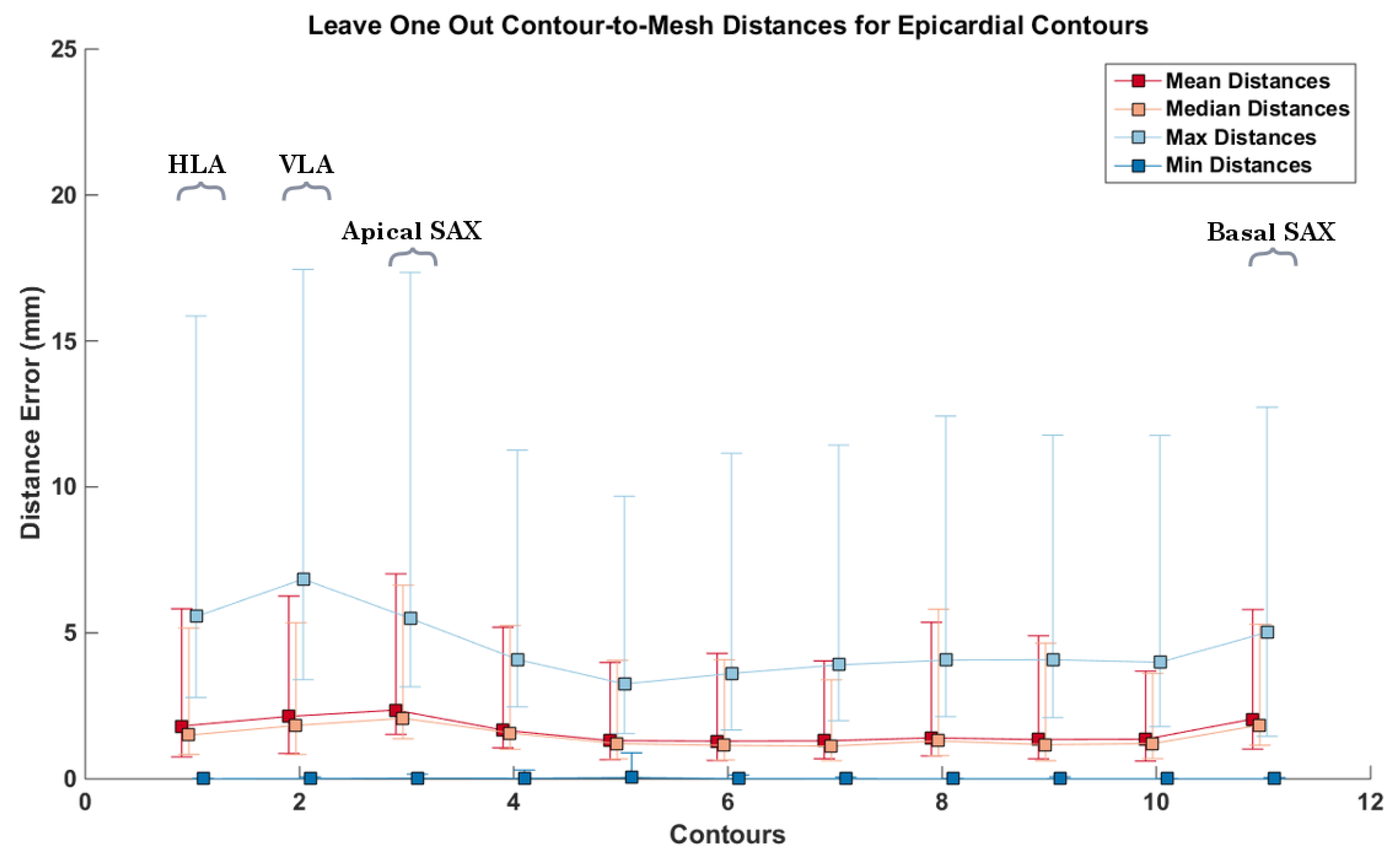
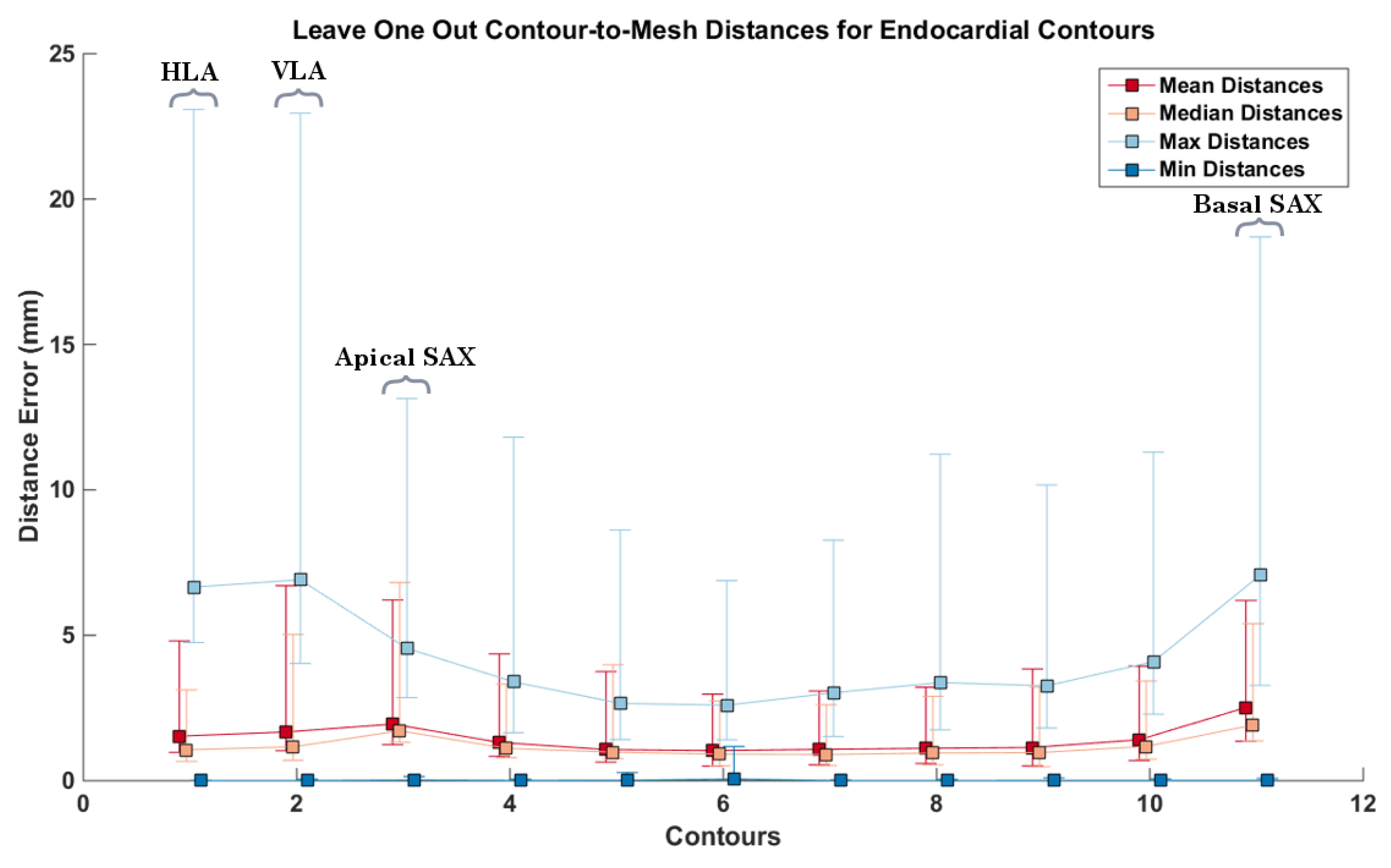
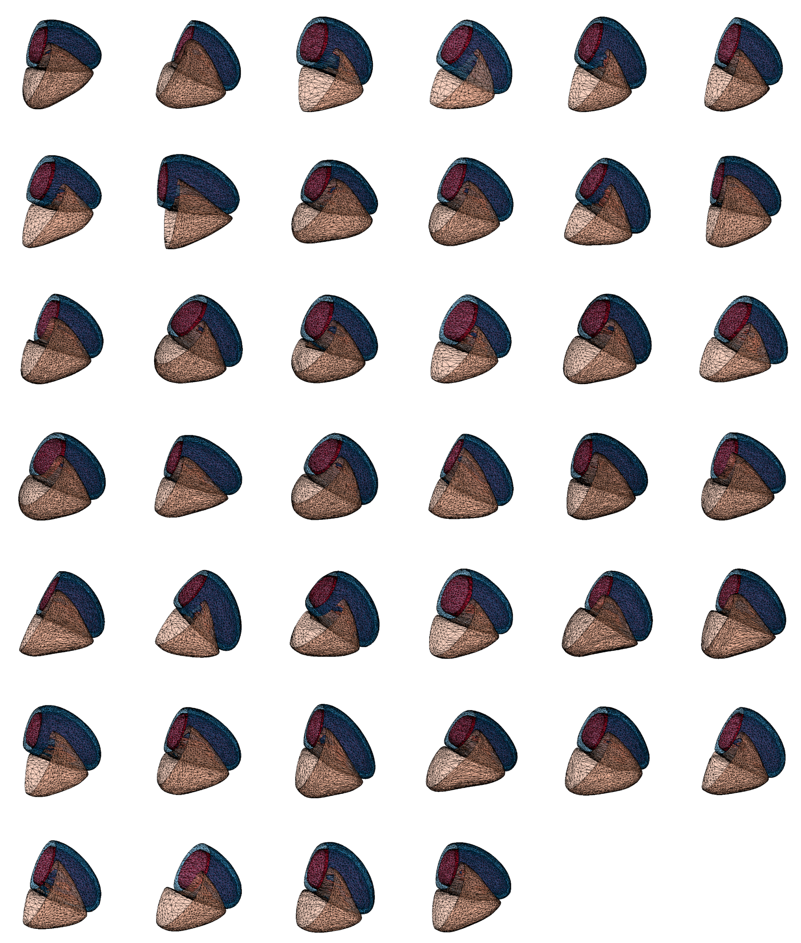
3.3. CMR Acquired Data

Our reconstruction was applied to real data to show how it responds to both normal and abnormal cases. As we use expert delineated contours to build the mesh, there is no ground truth to assess our method on. However, we performed quantitative analysis on the real datasets by measuring the discrepancy between individual contours and the resulting mesh (contour-to-mesh distance). This measurement provides an evaluation of the “goodness of fit” of the mesh with regards to the input contours. An example of this can be seen in Figure 10, as the blue box-plots (labelled O M ). Each blue box-plot represents the contour-to-mesh distance distributions for each respective contour. It should be noted that there is an inherent contour discrepancy brought by the non-coincidental nature of the contours. It can be seen that the resulting mesh has a distance no bigger then 2 mm to each of the contours. The example showed was performed on the epicardium of an abnormal case with severe myocardial thickening, as seen in Figure 8. This particular case was chosen as an example as we wanted a more complex geometry to demonstrate were the “fitting” effect would be noticeable. The resulting epicardial and endocardial surfaces can be observed in Figure 9.
To further evaluate the individual impact each contour has on the resulting mesh geometry, we calculated the error distance from each of the contours to the output mesh, having removed that specific contour prior to building the mesh, in a leave-one-out fashion. In performing this experiment, we assess the ability of our method to interpolate missing information from the dataset, as well as analyzing the structural and morphological information provided by each cardiac contour. The red box-plots (labelled C M ) in Figure 10 show the results applied to the same abnormal case (Figure 8). It can be observed that the contours where the highest amount of error occurred were the LAX, and the basal and apical slices. It can also be seen that the second contour left of the apical slice has a significant error when having the mesh generated without it. This is the region where myocardial thickening is most prevalent, as seen in Figure 8. We performed the same leave-one-out experiment on all 24 cases for the epi- and endocardium. The results can be seen in Figure 11. In order not to bias the experiment, we chose similarly sized hearts, each containing 11 images. As we obtain an error distance distribution for each of the contours, since each of the distance is the closest point-to-mesh distance for a contour, we calculated the mean, median, minimum and maximum distance values of each of the distributions. This resulted in 24 values for each of the statistical measurements. The squares and error bars on the graphs represent their distribution. From these graphs, it can be seen that, for the various normal and abnormal cases, the LAX along with the basal and apical slices are the slices where the distance error was more significant due to their structural information. This effect is more pronounced in the endocardium, as the geometry is more complex. It appears that the epicardium meshes rely more on the LAX and apical contours, whilst the endocardial meshes rely more on the information provided by the LAX and basal slices.

4. Discussion

To be able to assess various aspects of our methodology, several experiments were carried out, using both synthetic and real data.
One of the biggest hurdles in validating methodologies on real data is the lack of ground truth. This can be due to the intra-inter user segmentation differences causing spatial inconsistencies, or slice misalignment due to breath hold related issues, or simply because the acquisition is sparse, providing partial views or information from the whole underlying anatomy. Due to the partial volume effect when acquiring CMR slices, the gap between contoured slices are significant, as CMR slices are typically 8 mm thick and separated by a 2 mm gap, creating around 10 mm spacing between each contour. This inherent gap between contour planes causes for existing anatomical features to be unobtainable or unrecoverable. Usually, the information between the gaps are interpolated, in-painted, or filled using prior information of what the geometry is believed to be. For this reason, we chose to use an SSM so that we had the global geometrical information, so that we may use it as ground truth.
As we wanted to quantify the ability of our method to work on standard CRM acquired data, without biasing the results to other indirect measurements, we simulated contours having the same spatial planes as real data, mimicking a real acquisition without inter-contour discrepancies. Furthermore, using the SSM allows us to generate legitimate, population-based, heart shapes. This is the main reason why we decided to use an SSM to generate ground truth with fully accessible anatomies, and to evaluate how well, as well as which parameters are required, for our method to mimic the completion of the gaps from only the provided partial contour information. By having possible entire heart-like shapes, we were able to validate and tune our method for the specific task of building cardiac anatomies. Using these synthesized contours, which include multiple SAX and LAX, we assessed the error between the generated mesh and the ground truth mesh given various parameter combinations. We assessed a total of 3440 parameter samplings over 40 fitted ground truth shapes generated from the SSM. Figure 3, in Section 3.1, shows a parallel coordinate plot of the different parameters evaluated, and the resulting error metrics of the output results given those parameters. Assessing the combination of each parameter permutation allows for obtaining the most favourable set of parameters that result in the most similar shape given a set of contours. We define similar in terms of the shape that has the minimum mesh-to-mesh distance while maintaining a relatively low number of triangles. As such, our metrics of evaluation were the mean and medium mesh-to-mesh distances for each of the cases, as well as the number of triangles. Using the parallel coordinate plot allowed us to interactively select the parameter ranges of interest, which are highlighted in blue. These parameters were used as the default parameters for all of our resulting meshes.
We fitted an SSM to data acquired from a normal cohort, and generated contours from the resulting new shape at the same planes as the real contours. This experiment informs us on the ability to recover meshes from CMR acquired coincidental contours. Using these contours as inputs, we generated meshes, which can be seen in Figure A2 in Appendix B, and compared them to the fitted shape models. Table 1 shows the resulting statistical measures for all of the mesh-to-mesh distances for all of our output shapes. It can be seen that all of the mean and median values fall under sub-pixel accuracy. The maximum error distances show that the methodology performed worst on the right ventricles. As the right ventricles only had one horizontal long axis (which contains the four chambers of the heart), each of the right ventricles had one LAX contour. This long axis typically falls within one side of the right ventricle, and as such the most extreme distances were due to the geometrical information at the opposing areas only relying on the SAX information.
The method was applied to a stack of synthesized parallel contours and the result can be seen in Figure 4. In order to capture the discrepancy between the ground truth and the resulting mesh, mesh-to-mesh distances were calculated. It can be seen in Figure 4c that the maximum discrepancy is around 2.5 mm for a human heart size. This error is the distance between the ground truth shape and the reconstructed mesh’s most apical areas. As we do not have information at the apex due to the absence of LAX, it is expected that this is where the discrepancy would be highest. Elsewhere, distances appear no greater than 2 mm. To be able to assess the impact the amount of SAX contours have on the process, the distance between meshes was calculated by incrementing the number of equidistant SAX of the input data, in an iterative manner, starting with 2 SAX up to a stack of 15. The resulting box plot showing the distances can be seen in Figure 5. It can be observed that there is a considerable reduction of distance discrepancies up until eight slices, after which the decrease in the distances is not as notable. In this experiment, 8–9 slices represent an average CMR acquired dataset as a SAX stack has generally an inter-slice distance of 10 mm. The outliers make up the error distances at the base of the mesh, where no information was provided.
The impact that long axes have on the provided data was then assessed. A stack of four short axis slices were selected at equidistant positions from base to apex, and 1–7 long axes were iteratively added simulating a radially oriented CMR acquisition. We evaluated the distance errors (see Figure 6), which show that, as the amount of LAX increases, the error decreases. From the results, it can be seen that, after the addition of three LAX, there is negligible decrease in the error distances, as they all fall within 1 mm, which is of subpixel accuracy.
After assessing the SAX and LAX impact on the resulting meshes, we generated non-parallel, non-coincidental contours for both the left and right ventricle, as per Section 3.2.3. Due to breath-hold related issues, cardiac images are often misaligned, which must be corrected for, in order to minimize the coincidental discrepancy between contours. This step causes contours to lose their parallelism. Furthermore, as there also exist inherent contour discrepancies due to segmentation issues, there always remains slight contour-to-contour discrepancies in cross sectional pairs. Performing the experiment in Section 3.2.3 allowed us to assess our methodology’s robustness to cope with this type of data. It can be seen in Figure 7 that, at the contours’ planes, the contour-to-mesh discrepancy falls under 1.7 mm for the left ventricle epicardium and under 2.5 mm for the right ventricle endocardium. Despite having non-parallel, non-coincidental contours, the resulting meshes are visually pleasing.
Finally, real data was used, for both a normal and abnormal case. The contours for the abnormal case can be seen in Figure 8. The resulting meshes can be observed in Figure 9. To assess our method’s ability to deal with standard CMR acquired datasets, we measured the individual contour-to-mesh discrepancies, which can be seen in Figure 10. It can be seen that, when all the contours are used (blue box-plots), the discrepancy is within 2 mm for the abnormal case (Figure 10). As we proceed to iteratively remove a single contour, in a leave-one-out fashion, and rebuild the mesh, the distance for that excluded contour to the mesh increases. It can be seen that, when the most basal SAX is removed, there is a high discrepancy occurring when measuring the distance from that contour to the resulting mesh. As this is the most basal slice, this is expected as the basal slice contains important structural information about the global geometry of the heart. When the basal slice is removed, our process relies on the LAX to fill in the basal information, which can lead to an early closure of the basal part of the mesh, which might be at a lower geometrical position than the contour, leading to high discrepancy. The removal of contours allows us to assess the individual contributions of the contours to the geometrical result of the mesh. As such, it can be noted that, in the abnormal case (Figure 9), at the positions where the thickening is greatest, when the contours containing valuable information are removed, the discrepancy will be high, which is also the case for the apex. Figure 11 shows the same experiment performed on all 24 cases. It can be seen that the highest discrepancies occur for the endocardial surfaces. It can be noted that the apical slices for the epicardial contours are significantly higher, and, when removed, the same error measurement occurs as the long axes. Both mesh results from normal and abnormal anatomies were pooled in the results. As the epicardial surfaces are typically comprised of simpler anatomy with respect to the endocardial surfaces, when the apical contour was removed, only a few attractor points remained on the long axes, causing the mesh to not fully recover the underlying anatomy of the epicardial surface. With regards to the endocardial surfaces, as they are more complex, and the long axes can be quite convoluted in an abnormal anatomy, more attractor points are selected causing a lower contour-to-mesh error. These figures show that, even if the LAX contours are provided, the apical contour information should also be provided, in order to allow for a more accurate representation of the anatomy of the heart. Regardless, it can be seen that the main structural information is provided by the long axes contours. Furthermore, the information obtained from the most extremal slices is hard to interpolate, and causes the mesh to deviate from the underlying geometry, as opposed to the removal of a middle slice, which would not lead to a major loss of structural information. Our method does come with some drawbacks, notably the ability to cope with branching only if branching information has been provided in the initial mesh. Once the 3D surface meshes have been obtained, several clinical anatomical parameters relevant in the clinic can be acquired such as the ventricular volumes, wall thicknesses, or sphericity indices. Furthermore, volumetric meshes can easily be produced for electrophysiology or mechanical assessments in a biophysical simulations framework.

5. Conclusions

We presented a tool for surface reconstruction applicable to sparse, non-parallel, non-coincidental, heterogeneous cardiac contours. Our technique works on the left ventricle as well as on the right ventricle. We have empirically shown by means of the exposition of a variety of results that our technique results in reconstructed interpolating surfaces with very good fitting to the input contours. In the areas to be filled by the interpolated surfaces, our technique presents very pleasant visual appearance. We also show the importance of the LAX information and its effect on the resulting geometries, as well as introducing a new validation protocol that allows the evaluation of the various aspects of our methodology.

Acknowledgments

The authors would like to acknowledge Rina Ariga from the University of Oxford Centre for Clinical Magnetic Resonance Research, Division of Cardiovascular Medicine, Radcliffe Department of Medicine, University of Oxford, for providing CMR acquisitions, as well as Valentina Carapella from Simula Research Laboratory, Fornebu, Norway, for the segmentation of the data. B.V. acknowledges the support of the RCUK Digital Economy Programme grant number EP/G036861/1 (Oxford Centre for Doctoral Training in Healthcare Innovation). V.G. is supported by a BBSRC grant (BB/I012117/1), an EPSRC grant (EP/J013250/1) and by a BHF New Horizon Grant NH/13/30238. E.Z. acknowledges the Marie Skłodowska-Curie Individual Fellowship from the H2020 EU Framework Programme for Research and Innovation (Proposal No:655020-DTI4micro-MSCA-IF-EF-ST).

Author Contributions

B.V., V.G., and E.Z. conceived and designed the methods and experiments; B.V. and E.Z. performed the software implementation. B.V. wrote the paper. V.G. and E.Z. contributed to the editing and reviewing of the manuscript.

Conflicts of Interest

The authors declare no conflict of interest.

Abbreviations

The following abbreviations are used in this manuscript:
MRIMagnetic resonance imaging
CMRCardiac magnetic resonance
SAXShort axis slice
LAXLong axis slice
TPSThin plate spline
SSMStatistical shape model

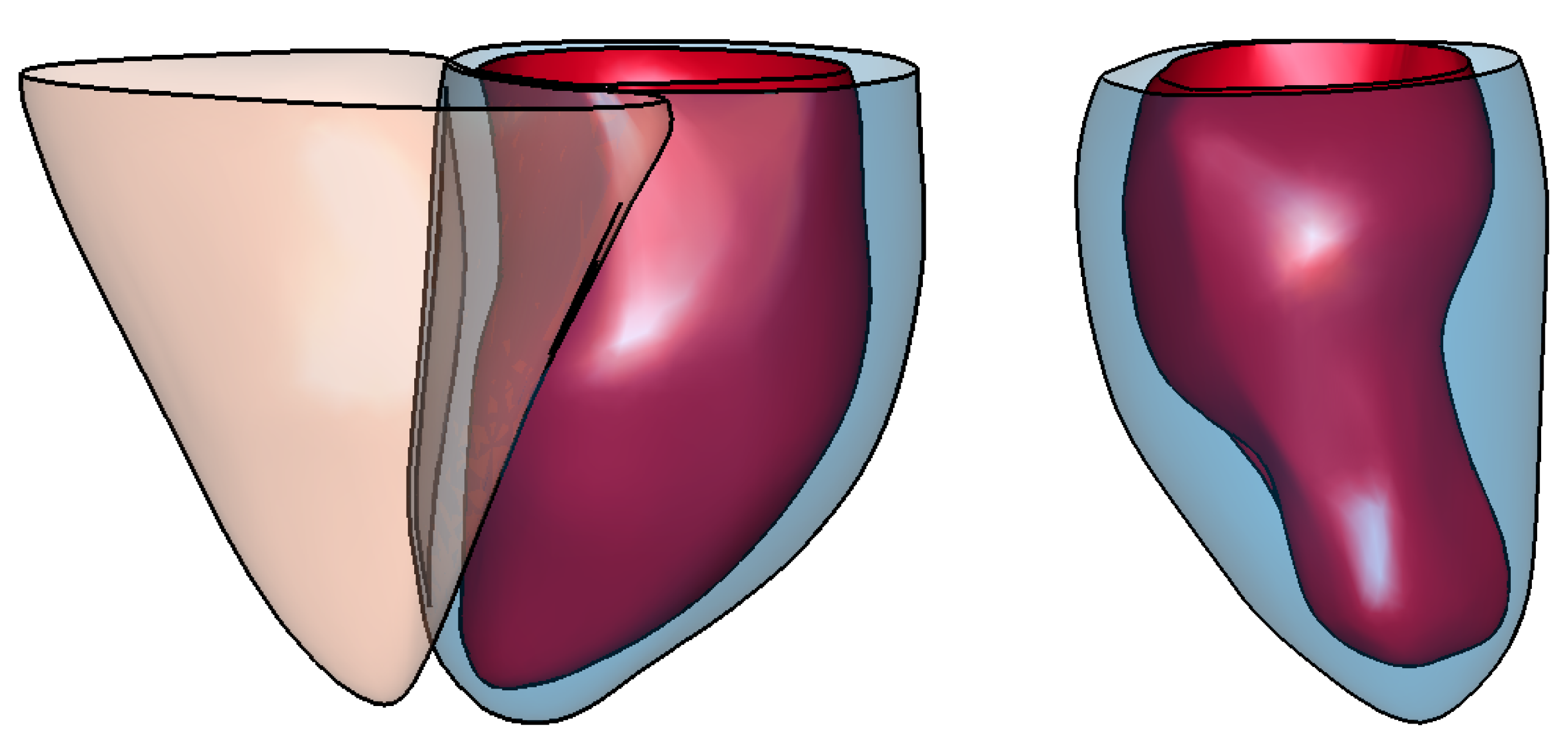
Appendix A. Illustration of Extreme Cases

In the exploration and tuning performed on the parameters of our method (see Section 3 and also Figure 3), several resulting meshes were obtained for the same input. Figure A1 illustrates some meshes for different extreme sets of parameters, generated from left epicardial contours.
Panel (a)—the mesh generated from the optimal parameters mentioned in Section 3 is shown.
Panel (b)—the mesh generated with a higher target reduction parameter in the decimation step, resulting in meshes with smaller numbers of triangles and vertices. Although visually pleasing and accurate for the case showed in the figure, the mesh can be seen to be more decimated, reducing the degrees of freedom, and restricting the method to tailor to abnormal cases.
Panel (c)—reduced amount of Laplacian smoothing iterations. This causes the geometrical structure of the mesh to be led more by the pulling process, creating more convoluted meshes, achieving meshes close to the contours, but with poor interpolation properties.
Panel (d)—mesh generated from a reduced amount of Laplacian smoothing iterations as well as lower sampling points. The mesh has therefore less attractor points on the contours, causing the mesh to become convoluted and have a higher contour to mesh distance discrepancy.
Panel (e)—mesh generated with a low value for the λ parameter in the approximate TPS step (see Equation (2)). This causes the mesh to become more elliptical and very smooth, as it has a high regularization weight with a low data matching weight. In addition, a large discrepancy with the contours can be observed.
Panel (f)—mesh generated with a low value of λ and a lower target reduction parameter. This causes the mesh to be smooth and elliptical, but with a high number of vertices. Similarly to (e), the mesh has a high contour to mesh distance.
Panel (g)—similarly to mesh (f) with a low Laplacian smoothing. This causes the high number of vertices to be pulled to the attractor points causing a convoluted appearance, although having a relatively low fitting error.
Figure A1. Illustration of resulting meshes for different extreme sets of parameters in the exploration and tuning of the parameters experiment. The color along the contours represents the distance to the resulting mesh. See the main text in Appendix A for comments on the different panels.
Jimaging 04 00016 g0a1

Appendix B. Simulation of CMR Acquisitions

Figure A2 shows the resulting meshes for the 40 simulated cases described in Section 3.1.
Figure A2. Resulting output mesh using our methodology on simulated CMR acquired contours (see Section 3.1). The figure shows the various shapes of the 40 generated meshes.
Jimaging 04 00016 g0a2

References

  1. Arevalo, H.; Vadakkumpadan, F.; Guallar, E.; Jebb, A.; Malamas, P.; Wu, K.; Trayanova, N. Arrhythmia risk stratification of patients after myocardial infarction using personalized heart models. Nat. Commun. 2016, 7, 11437. [Google Scholar] [CrossRef] [PubMed]
  2. Zou, M.; Holloway, M.; Carr, N.; Ju, T. Topology-Constrained Surface Reconstruction From Cross-sections. ACM Trans. Graph. 2015, 34, 128. [Google Scholar] [CrossRef]
  3. Sunderland, K.; Boyeong, W.; Pinter, C.; Fichtinger, G. Reconstruction of surfaces from planar contours through Contour interpolations. In Proceedings of the Image-Guided Procedures, Robotic Interventions, and Modeling, Orlando, FL, USA, 22–24 February 2015. [Google Scholar]
  4. Smith, N.; de Vecchi, A.; McCormick, M.; Nordsletten, D.; Camara, O.; Frangi, A.; Delingette, H.; Sermesant, M.; Relan, J.; Ayache, N.; et al. euHeart: Personalized and integrated cardiac care using patient-specific cardiovascular modelling. Interface Focus 2017, 1, 349–364. [Google Scholar] [CrossRef] [PubMed]
  5. Deng, D.; Zhang, J.; Xia, L. Three-Dimensional Mesh Generation for Human Heart Model. Life Syst. Model. Intell. Comput. 2010, 98, 157–162. [Google Scholar]
  6. Vukicevic, M.; Mosadegh, B.; Min, J.; Little, S. Cardiac 3D Printing and its Future Directions. JACC Cardiovasc. Imaging 2017, 10, 171–184. [Google Scholar] [CrossRef] [PubMed]
  7. Lehmann, H.; Kneser, R.; Neizel, M.; Peters, J.; Ecabert, O.; Kühl, H.; Kelm, M.; Weese, J. Integrating Viability Information into a Cardiac Model for Interventional Guidance. In Proceedings of the 5th International Conference Functional Imaging and Modeling of the Heart (FIMH), Nice, France, 3–5 June 2009; pp. 312–320. [Google Scholar]
  8. Young, A.; Cowan, B.; Thrupp, S.; Hedley, W.; DellItalia, L. Left Ventricular Mass and Volume: Fast Calculation with Guide-Point Modelling on MR Images. Radiology 2000, 2, 597–602. [Google Scholar] [CrossRef] [PubMed]
  9. Lamata, P.; Niederer, S.; Nordsletten, D.; Barber, D.; Roy, I.; Hose, D.; Smith, N. An accurate, fast and robust method to generate patient-specific cubic Hermite meshes. Med. Image Anal. 2011, 15, 801–813. [Google Scholar] [CrossRef] [PubMed]
  10. Albà, X.; Pereañez, M.; Hoogendoorn, C.; Swift, A.; Wild, J.; Frangi, A.; Lekadir, K. An algorithm for the segmentation of highly abnormal hearts using a generic statistical shape model. IEEE Trans. Med. Imaging 2016, 35, 845–859. [Google Scholar] [CrossRef] [PubMed]
  11. Villard, B.; Zacur, E.; Dall’Armellina, E.; Grau, V. Correction of Slice Misalignment in Multi-breath-hold Cardiac MRI Scans. In International Workshop on Statistical Atlases and Computational Models of the Heart. (Imaging and Modelling Challenges. STACOM 2016); Lecture Notes in Computer Science (LNCS); Springer: Cham, Switzerland, 2016; Volume 10124. [Google Scholar]
  12. Villard, B.; Carapella, V.; Ariga, R.; Grau, V.; Zacur, E. Cardiac Mesh Reconstruction from Sparse, Heterogeneous Contours. In Medical Image Understanding and Analysis. (MIUA 2017); Communications in Computer and Information Science; Springer: Cham, Germany, 2017; Volume 723. [Google Scholar]
  13. Lopez-Perez, A.; Sebastian, R.; Ferrero, J. Three-dimensional cardiac computational modelling: Methods, features and applications. BioMed. Eng. OnLine 2015, 14, 35. [Google Scholar] [CrossRef] [PubMed]
  14. Schall, O.; Samozino, M. Surface from scattered points. In Proceedings of the International Workshop on Semantic Virtual Environments, Villars, Switzerland, 16–18 March 2005; pp. 138–147. [Google Scholar]
  15. Berger, M.; Tagliasacchi, A.; Saversky, L.; Alliez, P.; Guennebaud, G.; Levine, J.; Sharf, A.; Silva, C. A survey of surface reconstruction from Points clouds. Comput. Graph. Forum 2017, 36, 301–329. [Google Scholar] [CrossRef]
  16. Khatamian, A.; Arabnia, H. Survey on 3D Surface Reconstruction. J. Inf. Process. Syst. 2016, 12, 338–357. [Google Scholar]
  17. Hoppe, H.; DeRose, T.; Duchamp, T.; McDonald, J.; Stuetzle, W. Surface Reconstruction from Unorganized Points. SIGGRAPH Comput. Graph. 1992, 26, 71–78. [Google Scholar] [CrossRef]
  18. Bernardini, F.; Mittleman, J.; Rushmeier, H.; Silva, C.; Taubin, G. The Ball-pivoting algorithm for surface reconstruction. IEEE Trans. Vis. Comput. Graph. 1999, 5, 349–359. [Google Scholar] [CrossRef]
  19. Lim, C.; Su, Y.; Yeo, S.; Ng, G.; Nguyen, V.; Zhong, L.; Tan, R.S.; Poh, K.K.; Chai, P. Automatic 4D Reconstruction of Patient-Specific Cardiac Mesh with 1-to-1 Vertex Correspondence from Segmented Contours Lines. PLoS ONE 2014, 9, e93747. [Google Scholar] [CrossRef] [PubMed]
  20. Liu, L.; Bajaj, C.; Deasy, J.; Ju, T. Surface Reconstruction from Non-parallel Curve Networks. Eurographics 2008, 27, 155–163. [Google Scholar] [CrossRef] [PubMed]
  21. Zhang, Z.; Konno, K.; Tokuyama, K. 3D Terrain Reconstruction Based on Contours. In Proceedings of the Ninth International Conference on Computer Aided Design and Computer Graphics, Hong Kong, China, 7–10 December 2005; pp. 325–330. [Google Scholar]
  22. Wang, Z.; Geng, N.; Zhang, Z. Surface Mesh Reconstruction Based on Contours. In Proceedings of the International Conference on Computational Intelligence and Software Engineering, Wuhan, China, 11–13 December 2009; pp. 325–330. [Google Scholar]
  23. Kazhdan, M.; Bolitho, M.; Hoppe, H. Poisson Surface Reconstruction. In Proceedings of the Eurographics Symposium on Geometry Processing, Cagliari, Sardinia, 26–28 June 2006. [Google Scholar]
  24. De Marvao, A.; Dawes, T.; Shi, W.; Minas, C.; Keenan, N.; Diamond, T.; Durighel, G.; Montana, G.; Rueckert, D.; Cook, S.; et al. Population-based studies of myocardial hypertrophy: High resolution cardiovascular magnetic resonance atlases improve statistical power. J. Cardiovasc. Magn. Reson. 2015, 16, 16. [Google Scholar] [CrossRef] [PubMed]
  25. Bai, W.; Shi, W.; de Marvao, A.; Dawes, T.; O’Regan, D.; Cook, S.; Rueckert, D. A bi-ventricular cardiac atlas built from 1000+ high resolution MR images of healthy subjects and an analysis of shape and motion. Med. Image Anal. 2015, 26, 133–145. [Google Scholar] [CrossRef] [PubMed]
  26. Gonzalez, J.G.; Arce, G.R. Optimality of the myriad filter in practical impulsive-noise environments. IEEE Trans. on Signal Process. 2001, 49, 438–441. [Google Scholar] [CrossRef]
  27. Moenning, C.; Dodgson, N.A. Fast marching farthest point sampling for implicit surfaces and point clouds. Comput. Lab. Tech. Rep. 2003, 565, 1–11. [Google Scholar]
  28. Rohr, K.; Stiehl, H.; Sprengel, R.; Buzug, T.; Weese, J.; Kuhn, M. Landmark-based elastic registration using approximating thin-plate splines. IEEE Trans. Med. Imaging 2001, 20, 526–534. [Google Scholar] [CrossRef] [PubMed]
  29. Sprengel, R.; Rohr, K.; Stiehl, H. Thin-Plate Sline Approximation for Image Registration. Eng. Med. Biol. Soc. 1996, 18, 1190–1191. [Google Scholar]
  30. Dyn, N.; Levine, D.; Gregory, J. A Butterfly Subdivision Scheme for Surface Interpolation with Tension Control. ACM Trans. Graph. 1990, 9, 160–169. [Google Scholar] [CrossRef]
  31. Nealen, A.; Igarashi, T.; Sorkine, O.; Alexa, M. Laplacian Mesh Optimization. In Proceedings of the 4th International Conference on Computer Graphics and Interactive Techniques in Australasia and Southeast Asia, Kuala Lumpur, Malaysia, 29 November–2 December 2006. [Google Scholar]
  32. Taubin, G. A signal processing approach to fair surface design. In Proceedings of the 22nd annual conference on Computer Graphics and Interactive Techniques, Los Angeles, CA, USA, 6–11 August 1995; pp. 351–358. [Google Scholar]
  33. Garland, M.; Heckbert, P. Surface simplification using quadric error metrics. In Proceedings of the 24th Annual Conference on Computer Graphics and Interactive Techniques, Los Angeles, CA, USA, 3–8 August 1997; pp. 209–216. [Google Scholar]
  34. McLeish, K.; Hill, D.L.G.; Atkinson, D.; Blackall, J.M.; Razavi, R. A study of the motion and deformation of the heart due to respiration. IEEE Trans. Med. Imaging 2002, 21, 1142–1150. [Google Scholar] [CrossRef] [PubMed]
  35. Shechter, G.; Ozturk, C.; Resar, J.R.; McVeigh, E.R. Respiratory motion of the heart from free breathing coronary angiograms. IEEE Trans. Med. Imaging 2004, 23, 1046–1056. [Google Scholar] [CrossRef] [PubMed]
Figure 1. An example of the SSM of the left ventricle epicardium and right ventricle endocardium fitted to real contours. The dark blue contours represent the real contours. The green contours represent the synthetic contours generated by slicing the SSM at the same spatial pose of the CMR acquired contour planes.
Jimaging 04 00016 g001
Figure 2. Overall pipeline for generating a surface mesh from contours illustrated on left epicardial contours. (a) the input contours; (b) tubular initial mesh with its vertices equally spaced along the contours; (c) the initial mesh after the Laplacian smoothing and showing the attractor points on the contours, with a visual illustration of their connections pulling the mesh; (d) the resulting mesh after several small deformations towards the attractor points; (e) the mesh after having undergone the process of subdivision, smoothing and decimation; (f) the resulting mesh, after several iteration of steps (d,e).
Jimaging 04 00016 g002
Figure 3. Parallel Coordinate graph showing the different combinations of parameters giving the minimum average, median, and min mesh to mesh distance, as well as the number of triangles generated. The red lines represent the selected bands for the y-axis. The highlighted blue lines represent the parameters that have generated meshes that satisfies the selected criteria. The faded lines represent every parameter permutation and their respective evaluation metrics. There are 3440 permutations. The fifth to seventh y-axis represent the mean, median and min mesh-to-mesh error distances in mm, between the ground truth meshes and the generated meshes given the respective parameters.
Jimaging 04 00016 g003
Figure 4. (a) the ground truth surface (left epicardium of the mean shape of the SSM) and the synthesized contours in red; (b) our resulting mesh given the red contours; (c) the surface-to-mesh distance error (in mm). The resulting mesh has been clipped at the level of the most basal contour.
Jimaging 04 00016 g004
Figure 5. Impact of increasing the number of SAX contours on the error distance between the generated mesh and the ground truth surface.
Jimaging 04 00016 g005
Figure 6. The effect of increasing the amount of left epicardial LAX contours have on the error distance between the generated mesh and the ground truth mesh. Top to bottom: 1–8 LAX slices added, successively. Each LAX added is a rotated version of the first LAX shown in the first row, first column. Rotations were generated as per the following: 90, 45, 135, 22.5, 157.5, 112.5, 67.5 degrees, respectively.
Jimaging 04 00016 g006
Figure 7. Distance map from the resulting geometrical mesh to the simulated cardiac input data. The contours were transformed by small out of plane rotations and translations. The left panel shows the resulting left ventricular epicardial mesh, and the right panel shows the right ventricular endocardial mesh. The distance errors represent the contour-to-mesh distances.
Jimaging 04 00016 g007
Figure 8. Different segmented CMR acquired contours on a severe abnormal anatomy.
Jimaging 04 00016 g008
Figure 9. Example of resulting surface meshes generated from (a) contours for a normal case, and (b) contours belonging to a severe abnormal anatomy. The left panel shows surface meshes for the left endocardial (in red) and epicardial (in blue) ventricle as well as the right epicardial ventricle (in orange). The right panel shows surface meshes for the left endocardial (in red) and epicardial (in blue) ventricle.
Jimaging 04 00016 g009
Figure 10. Endocardial contour-to-mesh distance having built the mesh with the entire set of contours (labelled O M , which stands for “Original Mesh”, in blue) and excluded contour-to-mesh distance having built the mesh without the excluded contour (labelled C M , which stands for “Computed Mesh”, in red).
Jimaging 04 00016 g010
Figure 11. Contour-to-mesh distances for all 24 cases, having built the meshes without the respectively excluded contour. Each error bar represents the distribution of distances for each of the respective statistical measurement. Each square represents the mean of each statistical measure, with the upper and lower notches representing the minimum and maximum values, respectively. Top: epicardial contour-to-mesh distances; bottom: endocardial contour-to-mesh distances. The y-axis represents the contour index. 1–2 represent the LAX, 3–11 represent the apex to the base, respectively.
Jimaging 04 00016 g011aJimaging 04 00016 g011b
Table 1. Table depicting the mesh-to-mesh distances (in mm) between the ground truth surface meshes and our generated meshes for 40 different geometries.
MeasureEpicardium (mm)Endocardium (mm)Right Ventricle (mm)
Mean0.120.140.29
Median0.090.090.22
Max1.111.293.34
Min1.35 × 10 5 2.04 × 10 5 7.49 × 10 5

