Improved Color Mapping Methods for Multiband Nighttime Image Fusion

Abstract

Previously, we presented two color mapping methods for the application of daytime colors to fused nighttime (e.g., intensified and longwave infrared or thermal (LWIR)) imagery. These mappings not only impart a natural daylight color appearance to multiband nighttime images but also enhance their contrast and the visibility of otherwise obscured details. As a result, it has been shown that these colorizing methods lead to an increased ease of interpretation, better discrimination and identification of materials, faster reaction times and ultimately improved situational awareness. A crucial step in the proposed coloring process is the choice of a suitable color mapping scheme. When both daytime color images and multiband sensor images of the same scene are available, the color mapping can be derived from matching image samples (i.e., by relating color values to sensor output signal intensities in a sample-based approach). When no exact matching reference images are available, the color transformation can be derived from the first-order statistical properties of the reference image and the multiband sensor image. In the current study, we investigated new color fusion schemes that combine the advantages of both methods (i.e., the efficiency and color constancy of the sample-based method with the ability of the statistical method to use the image of a different but somewhat similar scene as a reference image), using the correspondence between multiband sensor values and daytime colors (sample-based method) in a smooth transformation (statistical method). We designed and evaluated three new fusion schemes that focus on (i) a closer match with the daytime luminances; (ii) an improved saliency of hot targets; and (iii) an improved discriminability of materials. We performed both qualitative and quantitative analyses to assess the weak and strong points of all methods.

1. Introduction

The increasing availability and use of co-registered imagery from sensors with different spectral sensitivities have spurred the development of image fusion techniques [1]. Effective combinations of complementary and partially redundant multispectral imagery can visualize information that is not directly evident from the individual sensor images. For instance, in nighttime (low-light) outdoor surveillance applications, intensified visual (II) or near-infrared (NIR) imagery often provides a detailed representation of the spatial layout of a scene, while targets of interest like persons or cars may be hard to distinguish because of their low luminance contrast. While thermal infrared (IR) imagery typically represents these targets with high contrast, their background (context) is often washed out due to low thermal contrast. In this case, a fused image that clearly represents both the targets and their background can significantly enhance the situational awareness of the user by showing the location of targets relative to landmarks in their surroundings (i.e., by providing more information than either of the input images alone). Additional benefits of image fusion are a wider spatial and temporal coverage, decreased uncertainty, improved reliability, and increased system robustness.

Fused imagery that is intended for human inspection should not only combine the information from two or more sensors into a single composite image but should also present the fused imagery in an intuitive format that maximizes recognition speed while minimizing cognitive workload. Depending on the task of the observer, fused images should preferably use familiar representations (e.g., natural colors) to facilitate scene or target recognition or should highlight details of interest to speed up the search (e.g., by using color to make targets stand out from the clutter in a scene). This consideration has led to the development of numerous fusion schemes that use color to achieve these goals [2,3,4,5].

In principle, color imagery has several benefits over monochrome imagery for human inspection. While the human eye can only distinguish about 100 shades of gray at any instant, it can discriminate several thousand colors. By improving feature contrast and reducing visual clutter, color may help the visual system to parse (complex) images both faster and more efficiently, achieving superior segmentation into separate, identifiable objects, thereby aiding the semantic ‘tagging’ of visual objects [6]. Color imagery may, therefore, yield a more complete and accurate mental representation of the perceived scene, resulting in better situational awareness. Scene understanding and recognition, reaction time, and object identification are indeed faster and more accurate with realistic and diagnostically (and also—though to a lesser extent—non-diagnostically [7]) colored imagery than with monochrome imagery [8,9,10].

Color also contributes to ultra-rapid scene categorization or gist perception [11,12,13,14] and drives overt visual attention [15]. It appears that color facilitates the processing of color diagnostic objects at the (higher) semantic level of visual processing [10], while it facilitates the processing of non-color diagnostic objects at the (lower) level of structural description [16,17]. Moreover, observers can selectively attend task-relevant color targets and to ignore non-targets with a task-irrelevant color [18,19,20]. Hence, simply mapping multiple spectral bands into a three-dimensional (false) color space may already serve to increase the dynamic range of a sensor system [21]. Thus, it may provide immediate benefits such as improved detection probability, reduced false alarm rates, reduced search times, and increased capability to detect camouflaged targets and to discriminate targets from decoys [22,23].

In general, the color mapping should be adapted to the task at hand [24]. Although general design rules can be applied to assure that the information available in the sensor image is optimally conveyed to the observer [25], it is not trivial to derive a mapping from the various sensor bands to the three independent color channels. In practice, many tasks may benefit from a representation that renders fused imagery in realistic colors. Realistic colors facilitate object recognition by allowing access to stored color knowledge [26]. Experimental evidence indicates that object recognition depends on stored knowledge of the object’s chromatic characteristics [26]. In natural scene recognition, optimal reaction times and accuracy are typically obtained for realistic (or diagnostically) colored images, followed by their grayscale version, and lastly by their (nondiagnostically) false colored version [12,13,14].

When sensors operate outside the visible waveband, artificial color mappings inherently yield false color images whose chromatic characteristics do not correspond in any intuitive or obvious way to those of a scene viewed under realistic photopic illumination [27]. As a result, this type of false-color imagery may disrupt the recognition process by denying access to stored knowledge. In that case, observers need to rely on color contrast to segment a scene and recognize the objects therein. This may lead to a performance that is even worse compared to single band imagery alone [28,29]. Experiments have indeed demonstrated that a false color rendering of fused nighttime imagery which resembles realistic color imagery significantly improves observer performance and reaction times in tasks that involve scene segmentation and classification [30,31,32,33], and the simulation of color depth cues by varying saturation can restore depth perception [34], whereas color mappings that produce counter-intuitive (unrealistically looking) results are detrimental to human performance [30,35,36]. One of the reasons often cited for inconsistent color mapping is a lack of physical color constancy [35]. Thus, the challenge is to give night vision imagery an intuitively meaningful (‘realistic’ or ‘natural’) color appearance, which is also stable for camera motion and changes in scene composition and lighting conditions. A realistic and stable color representation serves to improve the viewer’s scene comprehension and enhance object recognition and discrimination [37]. Several different techniques have been proposed to render night-time imagery in color [38,39,40,41,42,43]. Simply mapping the signals from different nighttime sensors (sensitive in different spectral wavebands) to the individual channels of a standard RGB color display or to the individual components of a perceptually decorrelated color space (sometimes preceded by a principal component transform or followed by a linear transformation of the color pixels to enhance color contrast) usually results in imagery with an unrealistic color appearance [36,43,44,45,46]. More intuitive color schemes may be obtained by opponent processing through feedforward center-surround shunting neural networks similar to those found in vertebrate color vision [47,48,49,50,51,52,53,54,55]. Although this approach produces fused nighttime images with appreciable color contrast, the resulting color schemes remain rather arbitrary and are usually not strictly related to the actual daytime color scheme of the scene that is registered.

We, therefore, introduced a method to give fused multiband nighttime imagery a realistic color appearance by transferring the first order color statistics of color daylight images to the nighttime imager [41]. This approach has recently received considerable attention [3,5,56,57,58,59,60,61,62,63,64,65,66], and has successfully been applied to colorize fused intensified visual and thermal imagery [5,57,58,60,61,64], FLIR imagery [67], SAR and FLIR imagery [38], remote sensing imagery [68], and polarization imagery [63]. However, color transfer methods based on global or semi-local (regional) image statistics typically do not achieve color constancy and are computationally expensive.

To alleviate these drawbacks, we recently introduced a look-up-table transform-based color mapping to give fused multiband nighttime imagery a realistic color appearance [69,70,71]. The transform can either be defined by applying a statistical transform to the color table of an indexed false color night vision image, or by establishing a color mapping between a set of corresponding samples taken from a daytime color reference image and a multi-band nighttime image. Once the mapping has been defined, it can be implemented as a color look-up-table transform. As a result, the color transform is extremely simple and fast and can easily be applied in real-time using standard hardware. Moreover, it yields fused images with a realistic color appearance and provides object color constancy, since the relation between sensor output and colors is fixed. The sample-based mapping is highly specific for different types of materials in the scene and can therefore easily be adapted to the task at hand, such as optimizing the visibility of camouflaged targets. In a recent study [72], we observed that multiband nighttime imagery that has been recolored using this look-up-table based color transform conveys the gist of a scene better (i.e., to a larger extent and more accurately) than each of the individual infrared and intensified image channels. Moreover, we found that this recolored imagery conveys the gist of a scene just as well as regular daylight color photographs. In addition, targets of interest such as persons or vehicles were fixated faster [72].

In the current paper, we present and investigate various alterations on the existing color fusion schemes. We will compare various methods and come up with fusion schemes that are suited for different tasks: (i) target detection; (ii) discrimination of different materials; and (iii) easy, intuitive interpretation (using natural daytime colors).

2. Overview of Color Fusion Methods

Broadly speaking, one can distinguish two types of color fusion:

• Statistical methods, resulting in an image in which the statistical properties (e.g., average color, width of the distribution) match that of a reference image;
• Sample-based methods, in which the color transformation is derived from a training set of samples for which the input and output (the reference values) are known.

Both of these types of methods have their advantages and disadvantages. One advantage of the statistical methods is that they require no exact match of a multiband sample image to derive the color transformation, and an image showing a scene with similar content suffices to derive the color transformation. The outcome is a smooth transformation that uses a large part of the color space, which is advantageous for the discrimination of different materials, as it leads to a smooth transformation this method may also generalize better to untrained scenes. The downside is that, since no correspondence between individual samples is used (only statistical properties of the color distribution are used), it results in somewhat less naturalistic colors.

On the other hand, the sample-based method derives the color transformation from the direct correspondence between input sensor values and output daytime colors and therefore leads to colors that match the daytime colors well. Hence, this method requires a multiband image and a perfectly matching daytime image of the same scene. It can handle a highly nonlinear relationship between input (sensor values) and output (daytime colors). This also means that the transformation is not as smooth as that of the statistical method. Also, a limited part of the color range is used (available in the training set). Therefore, the discrimination of materials is more difficult than with the statistical method. We have seen [69] that it generalizes well to untrained scenes of a similar environment and sensor settings. However, it remains to be seen how well it generalizes to different scenes and sensor settings.

In this study we investigated new methods that combine the advantages of both types of methods. We are looking for methods that lead to improvement on military relevant tasks: intuitive, natural colors (for good situational awareness, easy and fast interpretation), good discriminability of materials, good detectability of (hot) targets and a fusion scheme that generalizes well to untrained scenes. Note that these properties may not necessarily be combined in a single fusion scheme. Depending on the task at hand different fusion schemes can be optimal (and selected). Therefore, we have designed three new methods based on the existing method, that focus on (i) naturalistic coloring; (ii) detection of hot targets; (iii) discriminability of materials.

In this study we use the imagery obtained by the TRI-band color low-light observation (TRICLOBS) prototype imaging system for a comparative evaluation of the different fusion algorithms [73,74]. The TRICLOBS system provides co-axially registered visual, NIR (near infrared), and LWIR (longwave infrared or thermal) imagery (for an example, see Figure 1). The visual and NIR supply information about the context, while the LWIR is particularly suited for depicting (hot) targets, and allows for looking through smoke. Images have been recorded with this system in various environments. This makes it possible to investigate how well a fusion scheme derived from one image (set) and reference (set) transfers to untrained images recorded in the same environment (and with the same sensor settings) to an untrained, new scene recorded in the same environment or in a different environment. The main training set consists of six images recorded in the MOUT (Military Operations in Urban Terrain) village of Marnehuizen in the Netherlands [74].

3. Existing and New Color Fusion Methods

In this section, we give a short description of existing color fusion methods, and present our proposals for improved color fusion mappings.

3.1. Existing Color Fusion Methods

3.1.1. Statistics Based Method

Toet [41] presented a statistical color fusion method (or SCF) in which the first order statistics of the color distribution of the transformed multiband sensor image (Figure 1d) is matched to that of a daytime reference color image (Figure 2a). In the proposed scheme the false color (source) multiband image representation and the daytime color reference (target) image are first transformed to the perceptually decorrelated quasi-uniform CIELAB (L*a*b*) color space. Next, the mean (–) and standard deviation (σ) of each of the color channels (L*, a*, b*) of the multiband source image are set to the corresponding values of the daytime color reference image as follows:

$$\begin{array}{l}{L}_s^{\ast \prime }=\frac{{\sigma }_t^{L^{\ast }}}{{\sigma }_s^{L^{\ast }}}(L_s^{\ast }-{\overline{L}}_s^{\ast })+{\overline{L}}_t^{\ast }\\ a_s^{\ast \prime }=\frac{{\sigma }_t^{a^{\ast }}}{{\sigma }_s^{a^{\ast }}}(a_s^{\ast }-{\overline{a}}_s^{\ast })+{\overline{a}}_t^{\ast }\\ b_s^{\ast \prime }=\frac{{\sigma }_t^{b^{\ast }}}{{\sigma }_s^{b^{\ast }}}(b_s^{\ast }-{\overline{b}}_s^{\ast })+{\overline{b}}_t^{\ast }\end{array}$$

(1)

Finally, the colors are transformed back to RGB for display (e.g., Figure 3a).

Another example of a statistical method is described by Pitié et al. [75]. Their method allows one to match the complete 3D distribution by performing histogram equalization in three dimensions. However, we found that various artifacts result when this algorithm is applied to convert the input sensor values (RGB) into the output RGB values of the daytime reference images (e.g., Figure 3b). It has to be noted that Pitié et al. [75] designed their algorithm to account for (small) color changes in daytime photographs, and therefore it may not apply to an application in which the initial image is formed by sensor values outside the visible range.

3.1.2. Sample Based Method

Hogervorst and Toet [70] have shown that a color mapping similar to Toet’s statistical method [41] can also be implemented as a color-lookup table transformation (see also [4]). This makes the color transform computationally cheap and fast and thereby suitable for real-time implementation. In addition, by using a fixed lookup-table based mapping, object colors remain stable even when the image content (and thereby the distributions of colors) changes (e.g., when processing video sequences or when the multiband sensor suite pans over a scene).

In the default (so-called color-the-night or CTN) sample-based color fusion scheme [70] the color mapping is derived from the combination of a multiband sensor image and a corresponding daytime reference image. Each pair of corresponding pixels in both images is used as a training sample. Therefore, the multiband sensor image and its daytime color reference image need to be perfectly matched (i.e., they need to represent the same scene and need to have the same pixel dimensions). An optimized color transformation between the input (multiband sensor values) and the output (the corresponding daytime color) can then be derived in a training phase that consists of the following steps (see Figure 4):

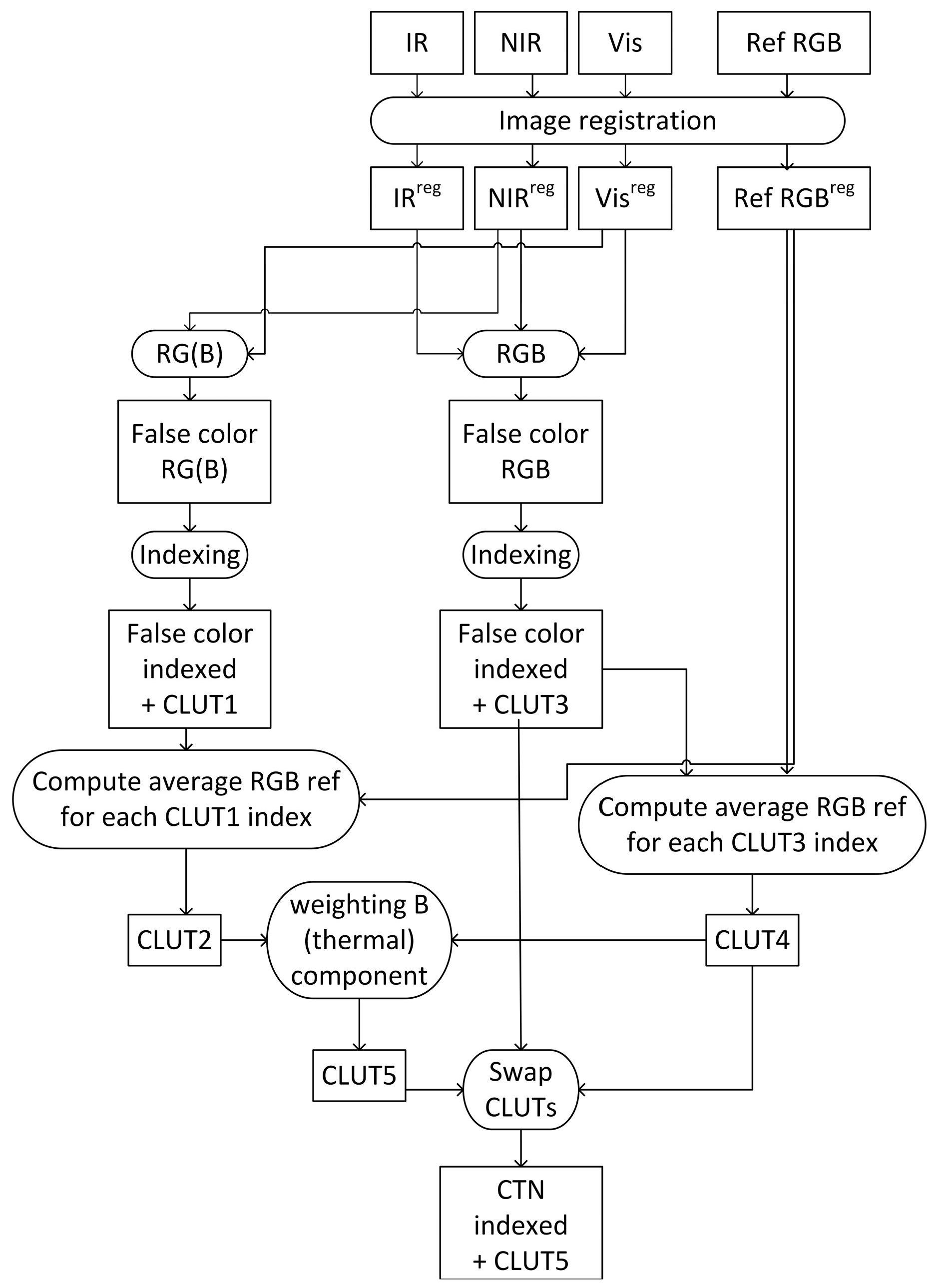
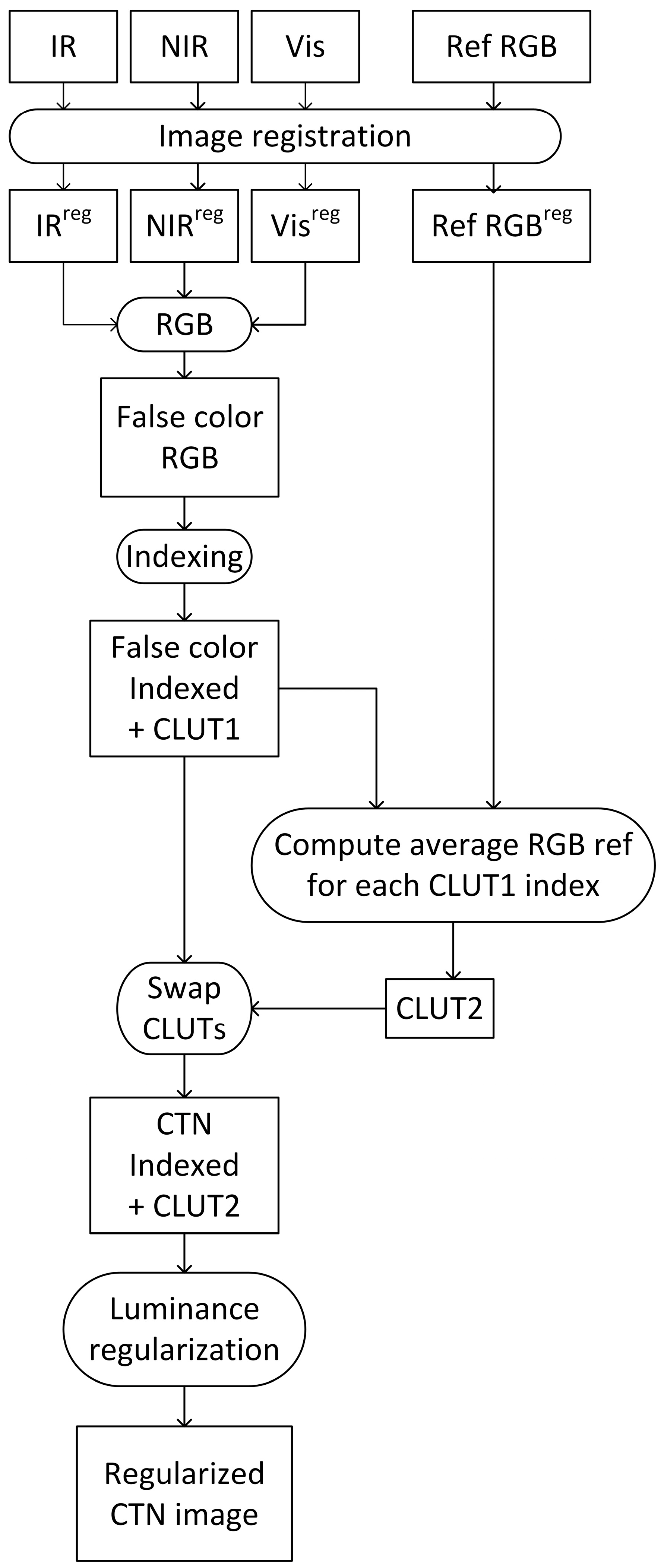
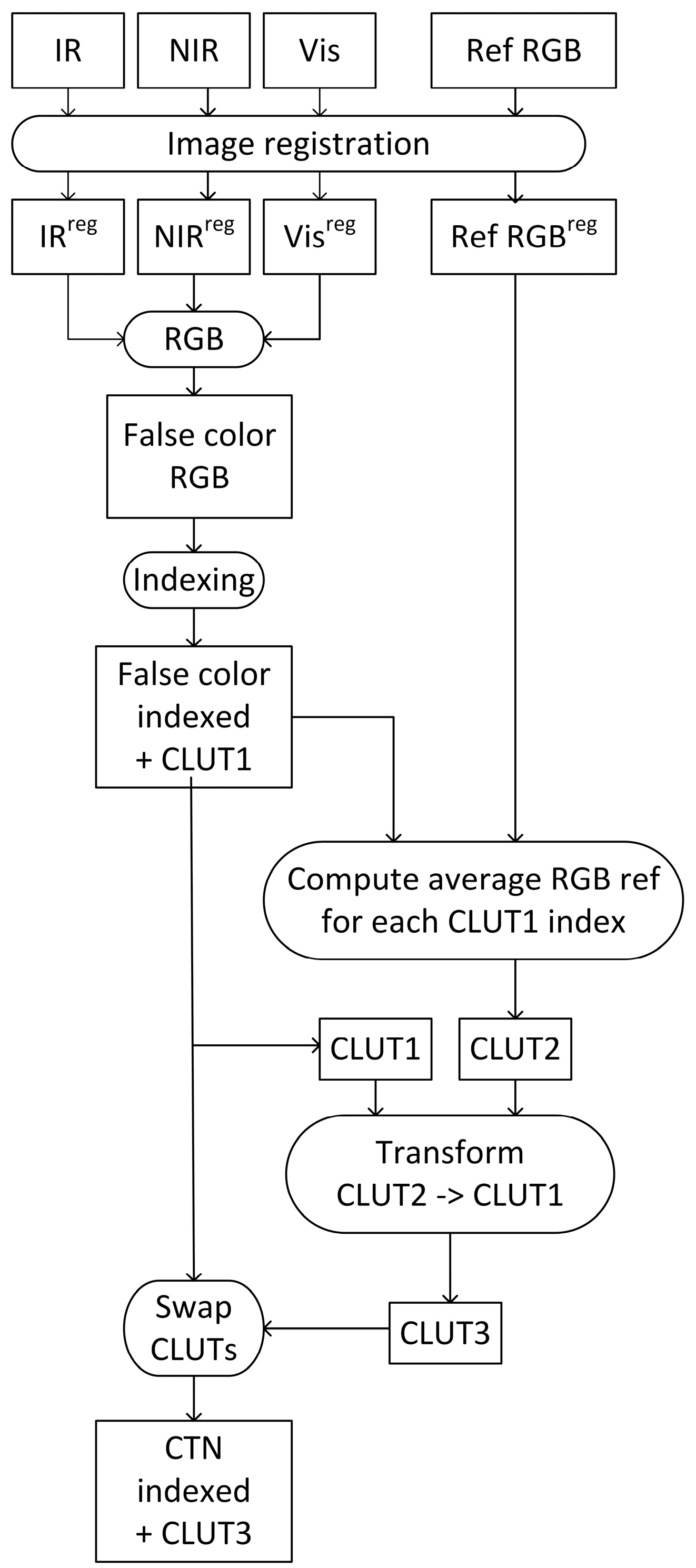
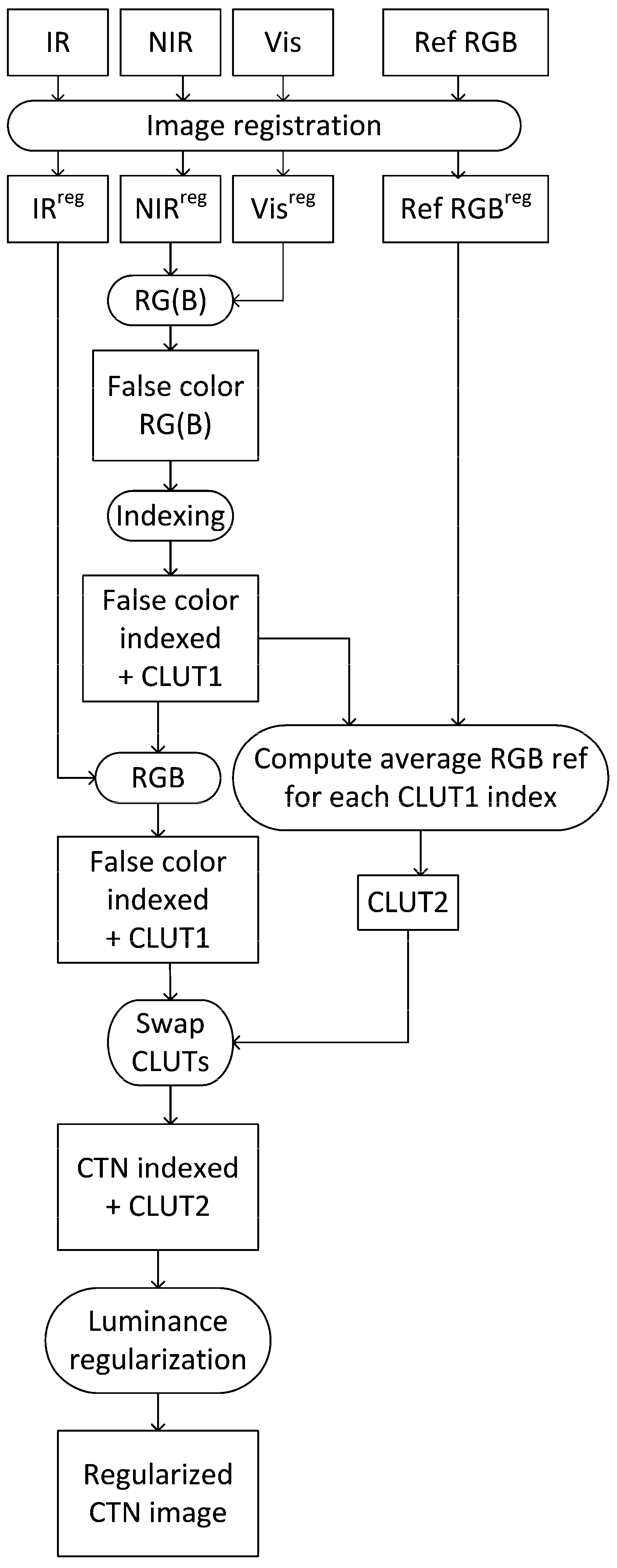
• The individual bands of the multiband sensor images and the daytime color reference image are spatially aligned.
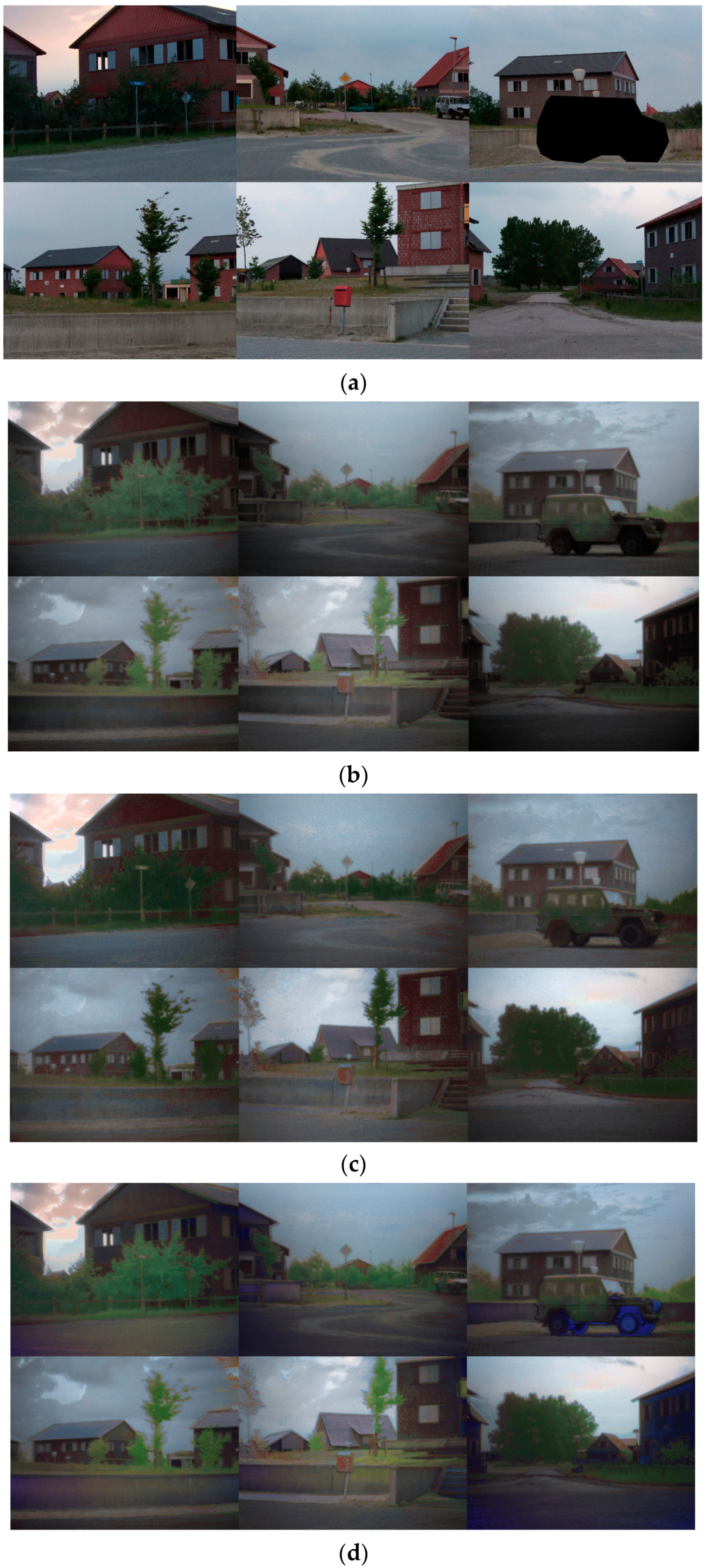
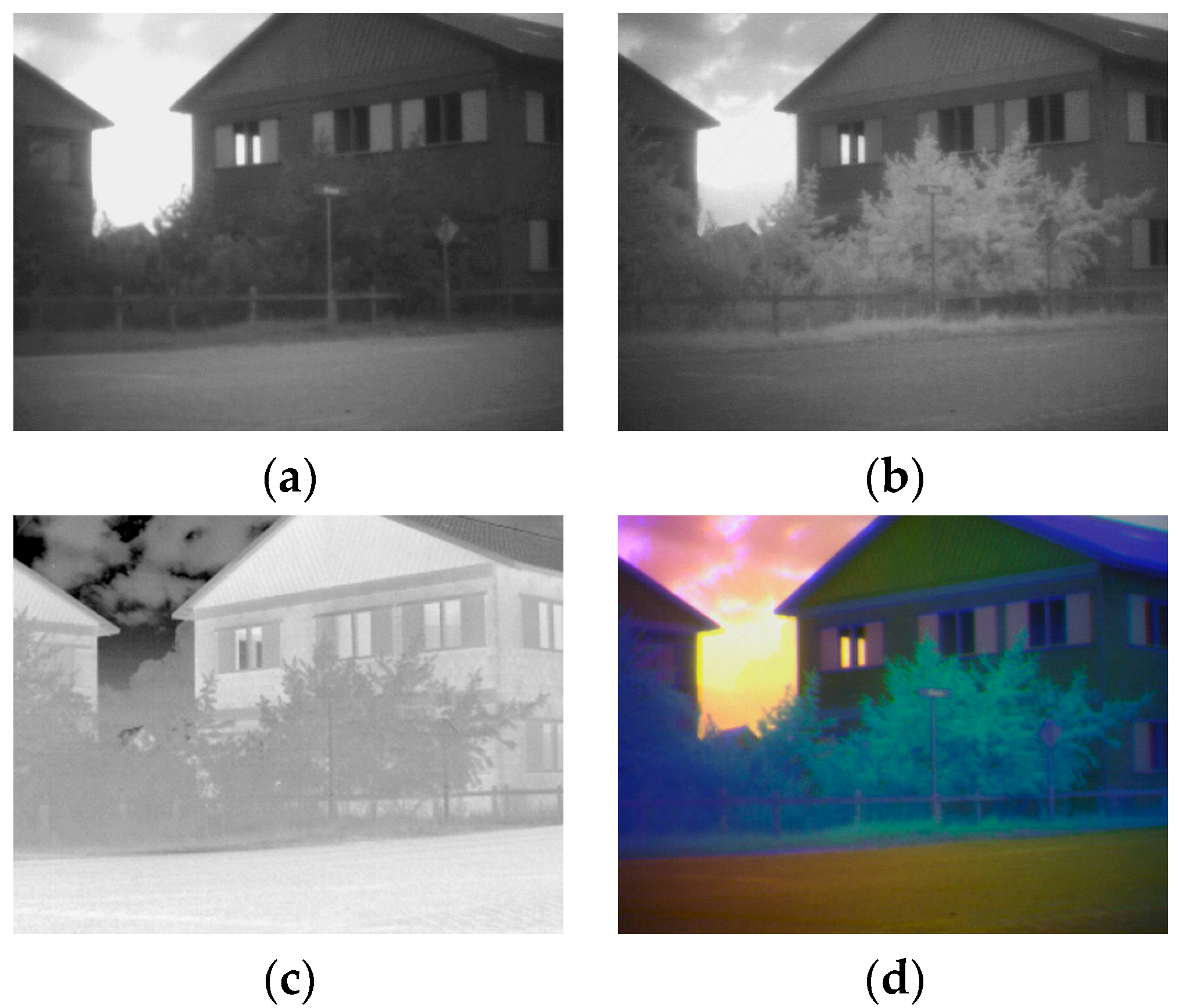
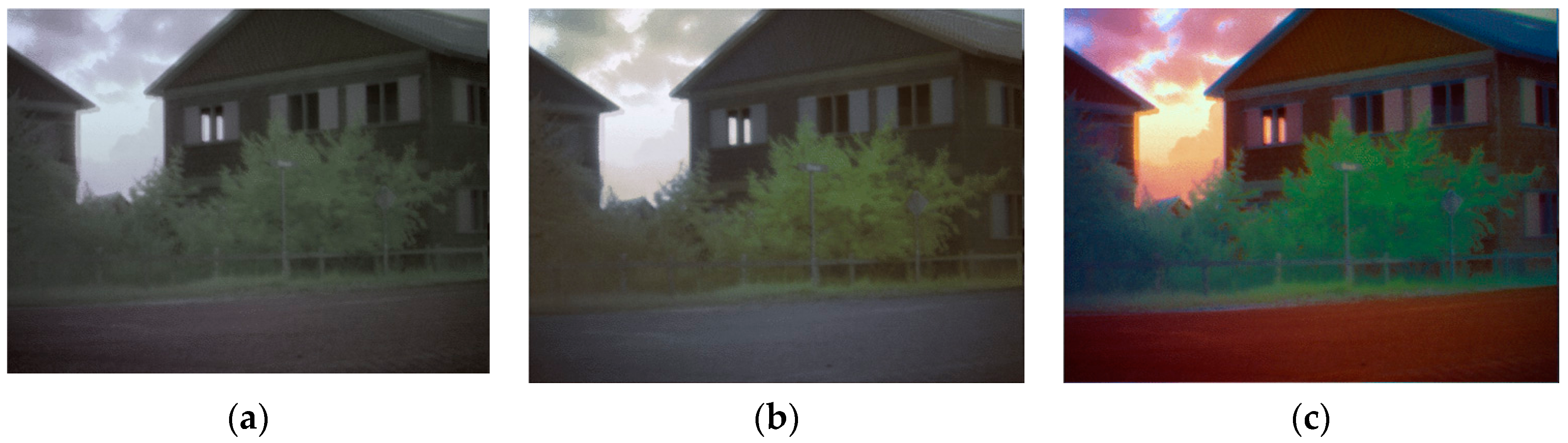
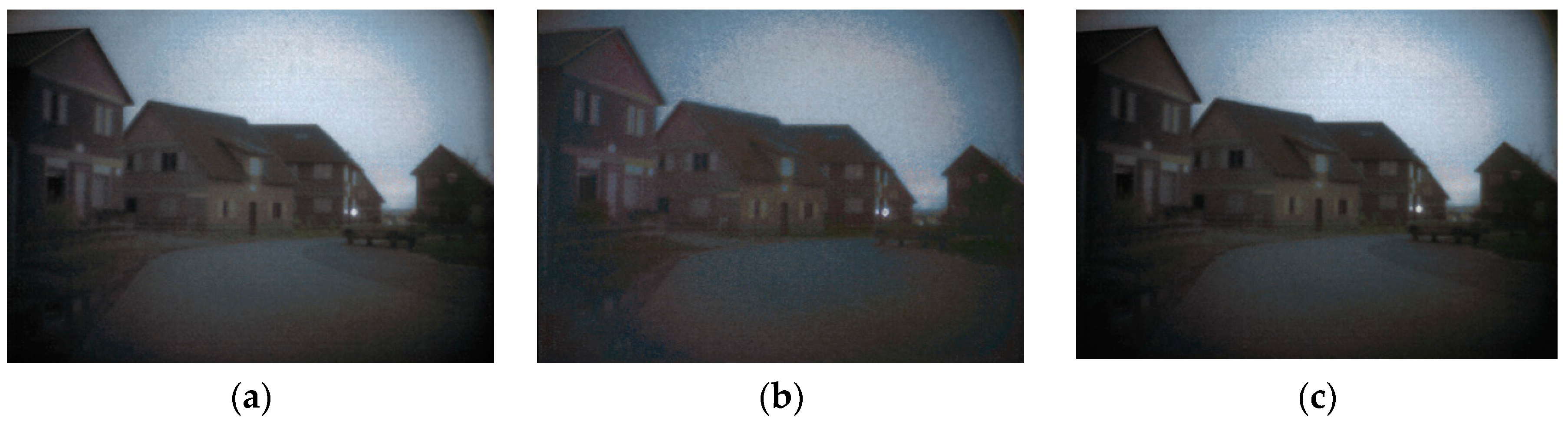
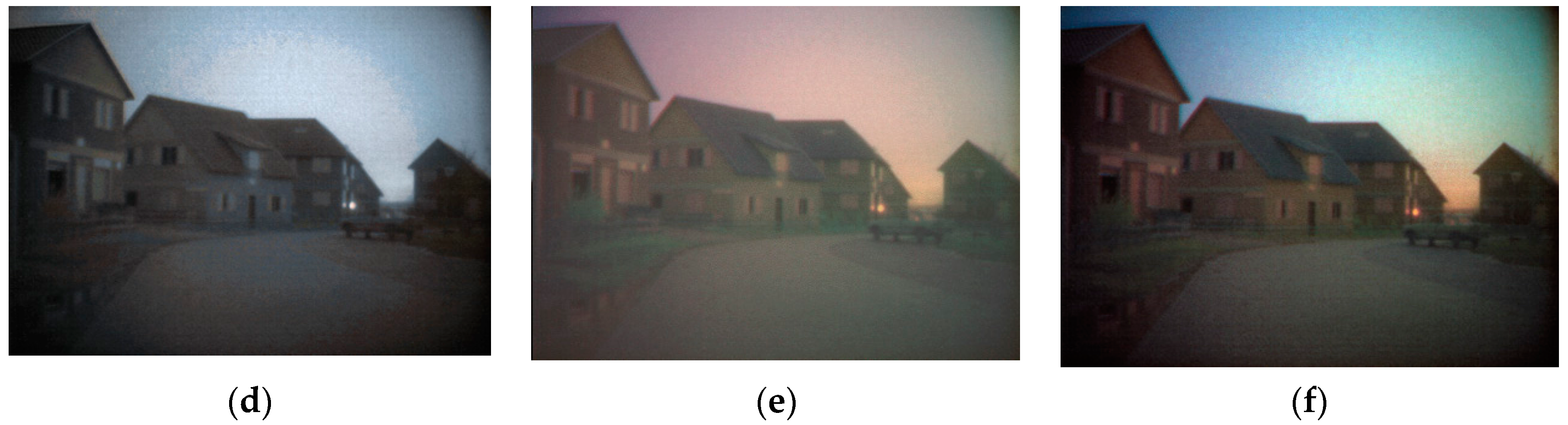
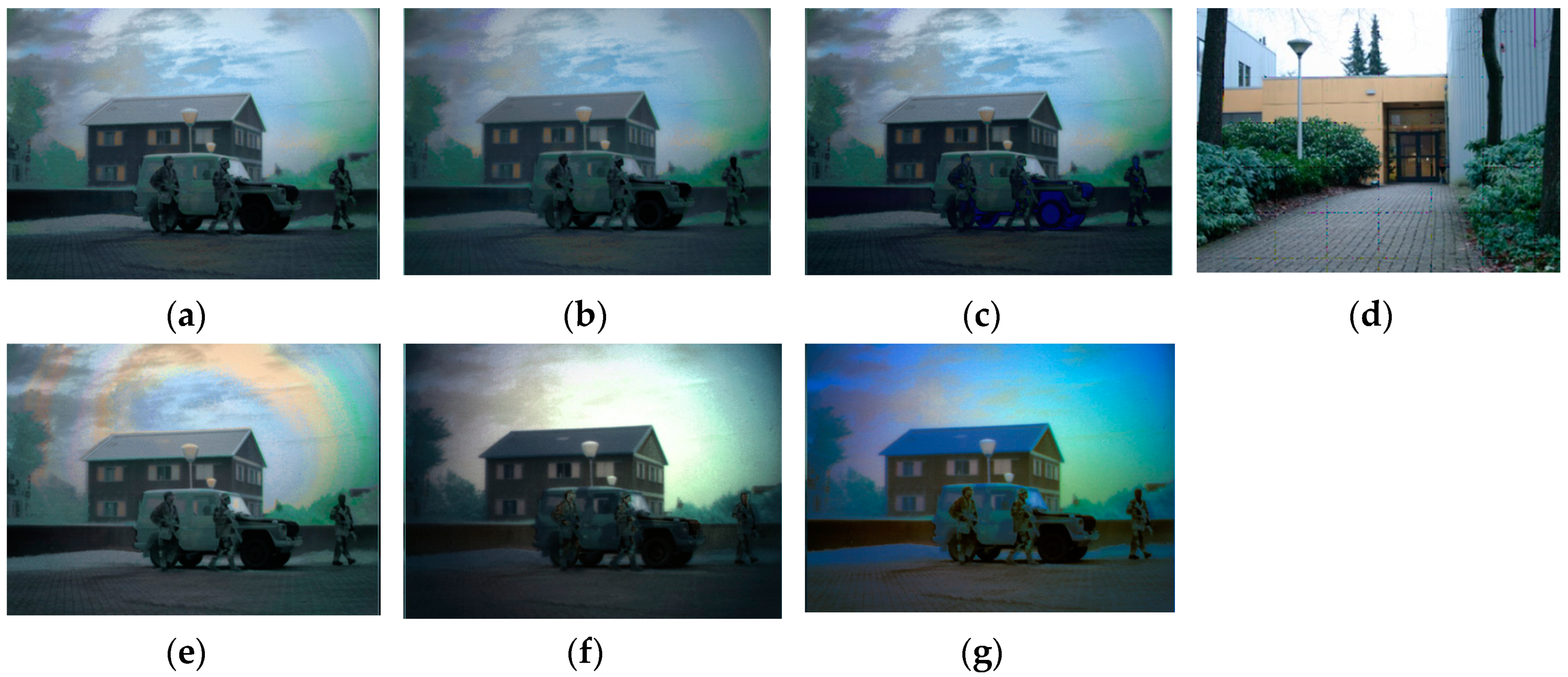
• The different sensor bands are fed into the R, G, B, channels (e.g., Figure 1d) to create an initial false-color fused representation of the multiband sensor image. In principle, it is not important which band feeds into which channel. This is merely a first presentation of the image and has no influence on the final outcome (the color fused multiband sensor image). To create an initial representation that is closest to the natural daytime image we adopted the ‘black-is-hot’ setting of the LWIR sensor.
• The false-color fused image is transformed to an indexed image with a corresponding CLUT₁ (color lookup table) that has a limited number of entries N. This comes down to a cluster analysis in 3-D sensor space, with a predefined number of clusters (e.g., the standard k-means clustering techniques may be used for implementation, thus generalizing to N-band multiband sensor imagery).
• A new CLUT₂ is computed as follows. For a given index d in CLUT₁ all pixels in the false-color fused image with index d are identified. Then, the median RGB color value is computed over the corresponding set of pixels in the daytime color reference image, and is assigned to index d. Repeating this step for each index in CLUT₁ results in a new CLUT₂ in which each entry represents the daytime color equivalent of the corresponding false color entry in CLUT₁. Thus, when $I=\{1,\dots ,N\}$ represents the set of indices used in the indexed image representation, and $d\in I$ represents a given index in I, then the support ${\mathrm{\Omega }}_d$ of d in the source (false-colored) image S is given by

  $${\mathrm{\Omega }}_d=\{\{i,j\}|\mathrm{Index}(S_{i,j})=d\}$$

  (2)

  and the new RGB color value $S_{i,j}^{\prime }$ for index d is computed as the median color value over the same support ${\mathrm{\Omega }}_d$ in the daytime color reference image R as follows:

  $$S_{i,j}^{\prime }=\mathrm{Median}\{\{R_{i,j}\}|\{i,j\}\in {\mathrm{\Omega }}_d\}$$

  (3)
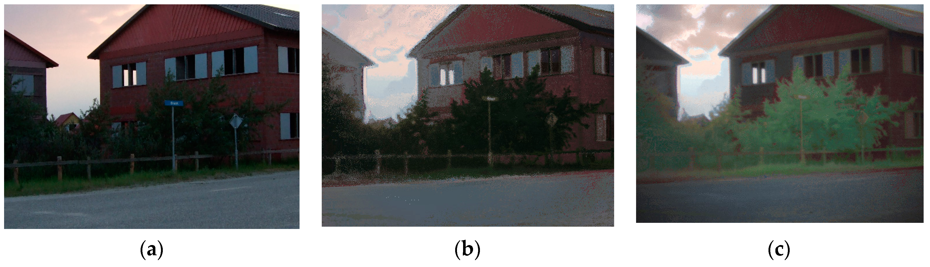
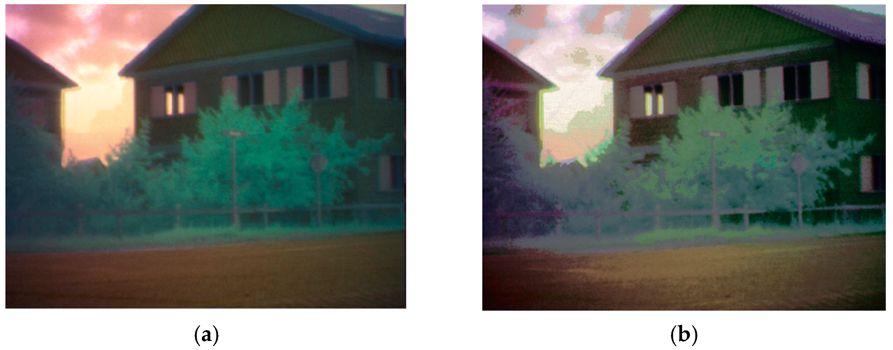
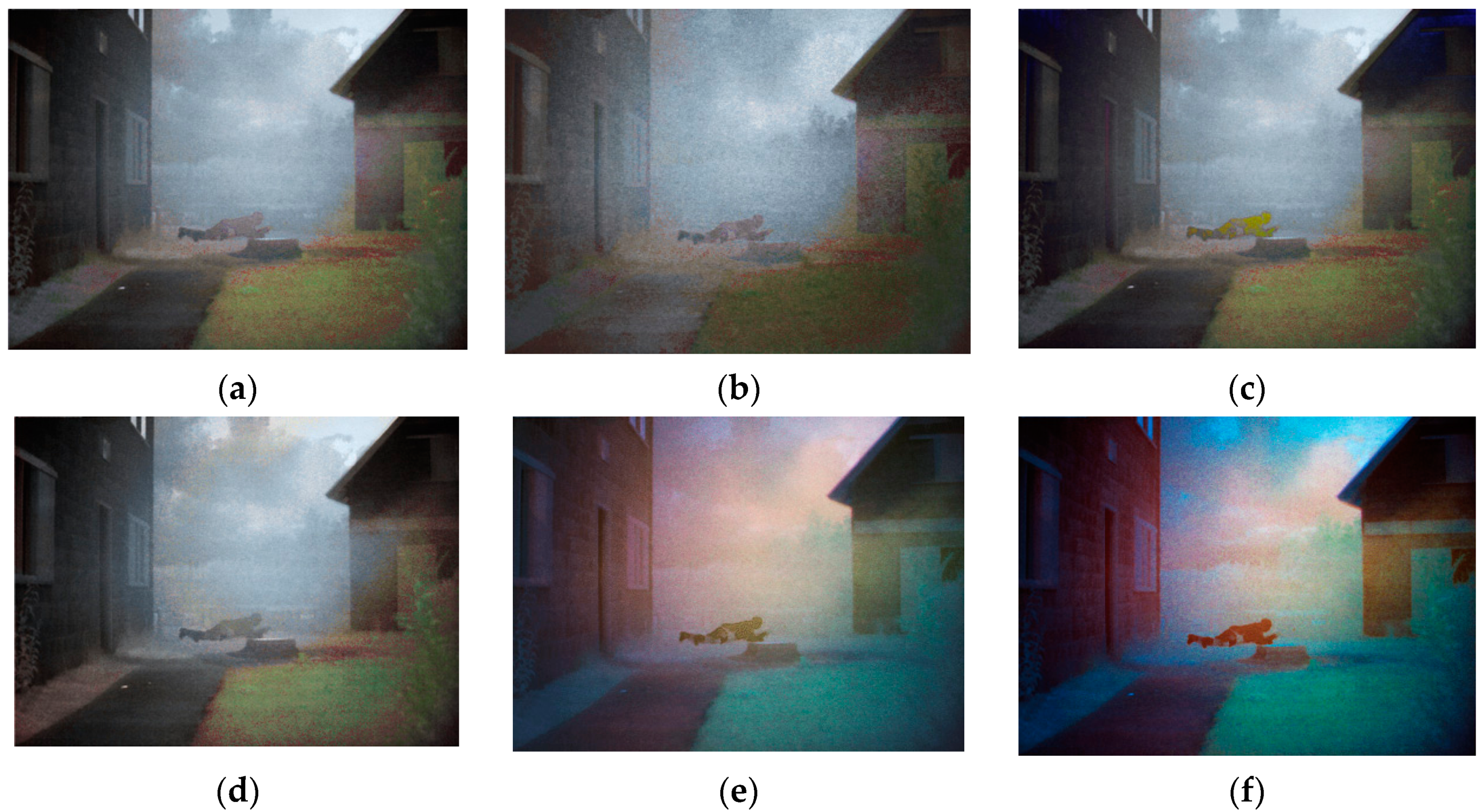
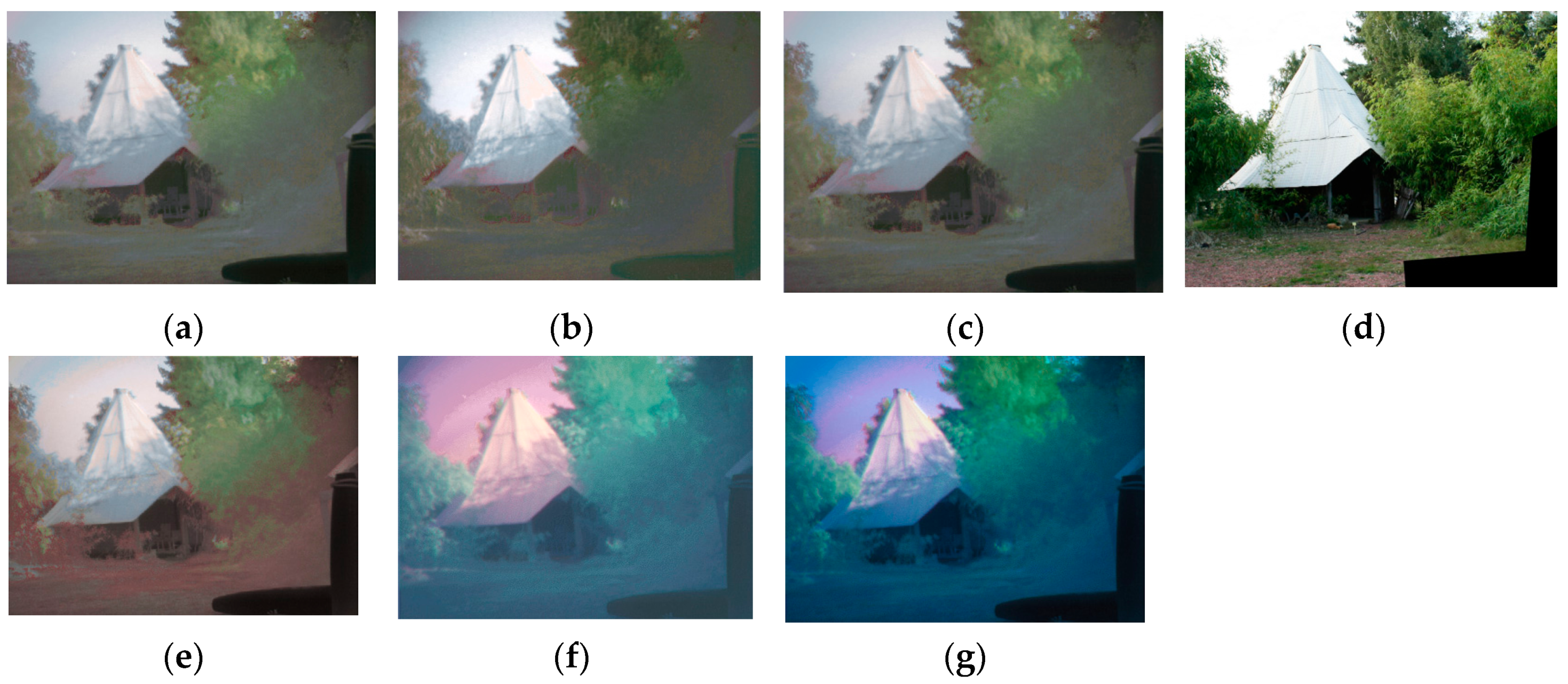
• The color fused image is created by swapping the CLUT₁ of the indexed sensor image to the new daytime reference CLUT₂. The result from this step may suffer from ‘solarizing effects’ when small changes in the input (i.e., the sensor values) lead to a large jump in the output luminance. This is undesirable, unnatural and leads to clutter (see Figure 2b).
• To eliminate these undesirable effects, a final step was included in which the luminance channel is adapted such that it varies monotonously with increasing input values. The luminance of the entry is thereto made proportional to the Euclidean distance in RGB space of the initial representation (the sensor values; see Figure 2c).

3.2. New Color Fusion Methods

3.2.1. Luminance-From-Fit

In the original CTN scheme, the luminance of the fused image was regularized using only on the input sensor values (see step 6, Section 3.1.2, and Figure 4). This regularization step was introduced to remove unwanted solarizing effects and to assure that the output luminance is a smooth function of the input sensor values. To make the appearance of the fused result more similar to the daytime reference image we derived a smooth luminance-from-fit (LFF) transformation between the input colors and the output luminance of the training samples. This step was implemented in the original CTN scheme as a transformation between two color lookup tables (the general processing scheme is shown Figure 5). Therefore, we converted the RGB data of the reference (daytime) image to HSV (hue, saturation, value) and derived a smooth transformation between input RGB colors and output value using a pseudo-inverse transform:

$$V=V_0+M\cdot x$$

(4)

where x’ = (r, g, b). We tried fitting higher polynomial functions as well as a simple linear relationship and found that the latter gave the best results (as judged by eye). The results of the LFF color fusion scheme derived from the standard training set and applied to this same set are depicted in Figure 6c. This figure shows that the LFF results show more resemblance with the daytime reference image (Figure 3a) than the result of the CTN method (Figure 6b). This is most apparent for the vegetation, which is darker in the LFF result than in the CTN fusion result, in line with the daytime luminance.

3.2.2. Salient-Hot-Targets

For situations in which it is especially important to detect hot targets, we derived a color scheme intended to make hot elements more salient while showing the environment in natural colors. This result was obtained by mixing the result from the CTN method (see Figure 7a) with the result from a two-band color transform (Figure 7b) using a weighted sum of the resulting CLUTs in which the weights depend on the temperature to the power 6 (see Figure 8 for the processing scheme of this transformation). This salient-hot-target (SHT) mapping results in colors that are the same as the CTN scheme except for hot elements, which are depicted in the color of the two-band system. We chose a mix with a color scheme that depends on the visible and NIR sensor values using the colors depicted in the inset of Figure 7b, with visible sensor values increasing from left to right, and NIR sensor values increasing from top to bottom. An alternative would be to depict hot elements in a color that does not depend on the sensor values of the visible and NIR bands. However, the proposed scheme also allows for discrimination between hot elements that differ in the values of the two other sensor bands.

3.2.3. Rigid 3D-Fit

In our quest for a smooth color transformation we first tried to fit an affine (linear) transformation to convert the input RGB triples $x$ into output RGB triples $y$:

$$y=M\cdot x+t$$

(5)

where $M$ is a linear transformation and t is a translation vector. However, although this resulted in a smooth transformation, it also gave images a rather grayish appearance (see Figure 9a). By introducing higher-order terms, the result was smoother (see Figure 9b) and approached the CTN result, but the range of colors that was used remained limited. This problem may be due to the fact that the range of colors in the training set (the reference daytime images) is also limited. As a result, only a limited part of the color space is used, which hinders the discrimination of different materials (and is undesirable). This problem may be solved by using a larger variety of training sets.

To prevent the transformation from leading to a collapse of the color space, we propose to use a 3D rigid transformation. We have fitted a rigid 3D transformation describing the mapping from the input values corresponding to the entries of the initial CLUT₁ to the values held in the output CLUT₂ (see step 4 in Section 3.1.2), by finding the rigid transformation (with rotation R and translation t) that best describes the relationship (with $\zeta$ a deviation term that is minimized) using the method described by Arun et al. [76]:

$${\mathrm{CLUT}}_2=t+R\cdot {\mathrm{CLUT}}_1+\zeta$$

(6)

Next, the fitted values of the new CLUT₃ were obtained by applying the rigid transformation to the input CLUT₁:

$${\mathrm{CLUT}}_3=t+R\cdot {\mathrm{CLUT}}_1$$

(7)

As in the LFF method, this step was implemented in the original CTN scheme as a transformation between two color lookup tables (the general processing scheme is shown in Figure 5). Figure 9c shows an example in which the rigid-3D-fit (R3DF) transformation has been applied. Figure 10b shows the results obtained by applying the fitted 3-D transformation derived from the standard training set to the test set, which are the same in this case. The result shows some resemblance with the result of the statistical method (Figure 10a). However, R3DF results in a broader range of colors, and therefore a better discriminability of different materials. The colors look somewhat less natural than those resulting from the CTN method (Figure 6b). An advantage of the R3DF method over the SCF statistical method is that the color transformation is derived from a direct correspondence between the multiband sensor values and the output colors of individual samples (pixels), and therefore does not depend on the distribution of colors depicted in the training scene.

4. Qualitative Comparison of Color Fusion Methods

First, we performed a qualitative comparison between the different color fusion schemes. In our evaluation we included the CTN method (Figure 6b), the SCF method (Figure 10a), and the three newly proposed schemes: (1) the LFF method (see Figure 6c); (2) the SHT method (Figure 6d); and (3) the R3DF method (Figure 10b). We also included the result of the CTN method using only two input bands: the visible and the NIR band (CTN2: for the processing scheme see Figure 11). This last condition was added to investigate whether the colors derived from this two-band system transfer better to untrained scenes than when the LWIR band is used as well. The idea behind this is that only bands close to the visible range can be expected to show some correlation with the visible daytime colors. However, the LWIR values are probably relatively independent of the daytime color and therefore may not help in inferring the daytime color (and may even lead to unnatural colors). Next, we present some examples of the various images that were evaluated.

Figure 6 and Figure 7 show the results of the various color methods that were derived from the standard training set (of six images) and were applied to multiband images of the same scenes (except for the two-band system). In line with our expectations, the LFF method (Figure 6c) leads to results that are more similar to the daytime reference image (Figure 6a), with for instance vegetation shown in dark green instead of in light green in the CTN scheme (Figure 6b). As intended, the SHT method (Figure 6d) leads to hot elements (the engine of the vehicle) depicted in bright blue, which makes them more salient and thus easier to detect. The elements are shown in blue because the sensor values in the visible and NIR bands are close to zero in this case. The result of the R3DF method are shown in Figure 10b. As mentioned before, in this case, the results show some resemblance with the statistical method. However, the colors are more outspoken, due to the fact that the range of colors is not reduced in the transformation. Therefore, the discriminability of materials is quite good. The downside is that the colors are somewhat less natural than the CTN result (Figure 6b), although they are still quite intuitive. Figure 12 shows an example in which the color transformations derived from the standard training set were applied to a new (untrained) scene taken in the same environment. As expected, the CTN scheme transfers well to the untrained scene. Again, the LFF result matches the daytime reference slightly better than the CTN scheme, and the R3DF result shows somewhat less natural colors, but still yields good discriminability of the different materials in the scene. Surprisingly, the two-band system (Figure 12e) does not lead to more naturalistic colors than the three-band (CTN) method (Figure 12a).

Figure 13 shows yet another example of applying the methods to an image that was taken in the same environment but not used in the training set. In this case, the light level was lower than the levels that occur in the training set, which also led to differences in the sensor settings. No daytime reference is available in this case. Most of the color fusion methods lead to colors that are less outspoken. Again, the colors in the R3DF result are the most vibrant and lead to the best discriminability of materials. Figure 14 shows an example in which the SHT method leads to a yellow hot target, due to the fact that the sensor values in the visible and NIR bands are both high (see the inset Figure 7b for the color scheme that was used). In this case this leads to lower target saliency, since the local background is white. This indicates that this method is not yet optimal for all situations.

Figure 15 shows an example in which the color transformations were applied to an image recorded in a totally different environment (and with different sensor settings). Again, the CTN method transfers quite well to this new environment, while the two-band method performs less well. Finally, Figure 16 shows the results of applying the different color mapping schemes to a multiband image recorded in the standard environment, after they were trained on scenes representing a different environment (see Figure 16d). In this case, the resulting color appearance is not so natural as when the mapping schemes were trained in the same environment (see e.g., Figure 7a,c). Also here, the R3DF method (Figure 16g) appears to transfer well to this untrained situation (environment and sensor settings).

5. Quantitative Evaluation of Color Fusion Methods

To quantitatively compare the performance of the different color fusion schemes discussed in this study we performed both a subjective ranking experiment and a computational image quality evaluation study. Both evaluation experiments were performed with the same set of 138 color fused multiband images. These images were obtained by fusing 23 three-band (visual, NIR, LWIR) TRICLOBS images (each representing a different scene, see [74]) with each of the six different color mappings investigated in this study (CTN, CTN-2 band, statistical, luminance-from-fit, salient-hot-targets, and rigid-3D-fit).

5.1. Subjective Ranking Experiment

5.1.1. Methods

Four observers (two males and two females, aged between 31 and 61) participated in a subjective evaluation experiment. The observers had (corrected to) normal vision and no known color deficiencies. They were comfortably seated at a distance of 50 cm in front of a Philips 231P4QU monitor that was placed in a dark room. The images were 620 × 450 pixels in size, and were presented on a black background with a size of 1920 × 1080 pixels in a screen area of 50.8 × 28.8 cm². For each scene, the observers ranked its six different fused color representations (resulting from the six different color fusion methods investigated in this study) in terms of three criteria: image naturalness (color realism, how natural the image appears), discriminability (the amount of different materials that can be distinguished in the image), and the saliency of hot targets (persons, cars, wheels, etc.) in the scene. The resulting rank order was converted to a set of scores, ranging from 1 (corresponding to the worst performing method) to 6 (denoting the best performing method). The entire experiment consisted of three blocks. In each block, the same ranking criterium was used (either naturalness, discriminability or saliency) and each scene was used only once. The presentation order of the 23 different scenes was randomized between participants and between blocks. On each trial, a different scene was shown and the participant was asked to rank order the six different color representations of that given scene from “best performing” (leftmost image) to “worst performing” (rightmost image). The images were displayed in pairs. The participant was instructed to imagine that the display represented a window showing two out of six images that were arranged on a horizontal row. By selecting the right (left) arrow on the keyboard the participant could slide this virtual window from left to right (vice versa) over the row of images, corresponding to higher (lower) ratings. By pressing the up-arrow the left-right order of the two images on the screen could be reversed. By repeatedly comparing successive image pairs and switching their left-right order the participant could rank order the entire row of six images. When the participant was satisfied with the result, he/she pressed the Q-key to proceed to the next trial.

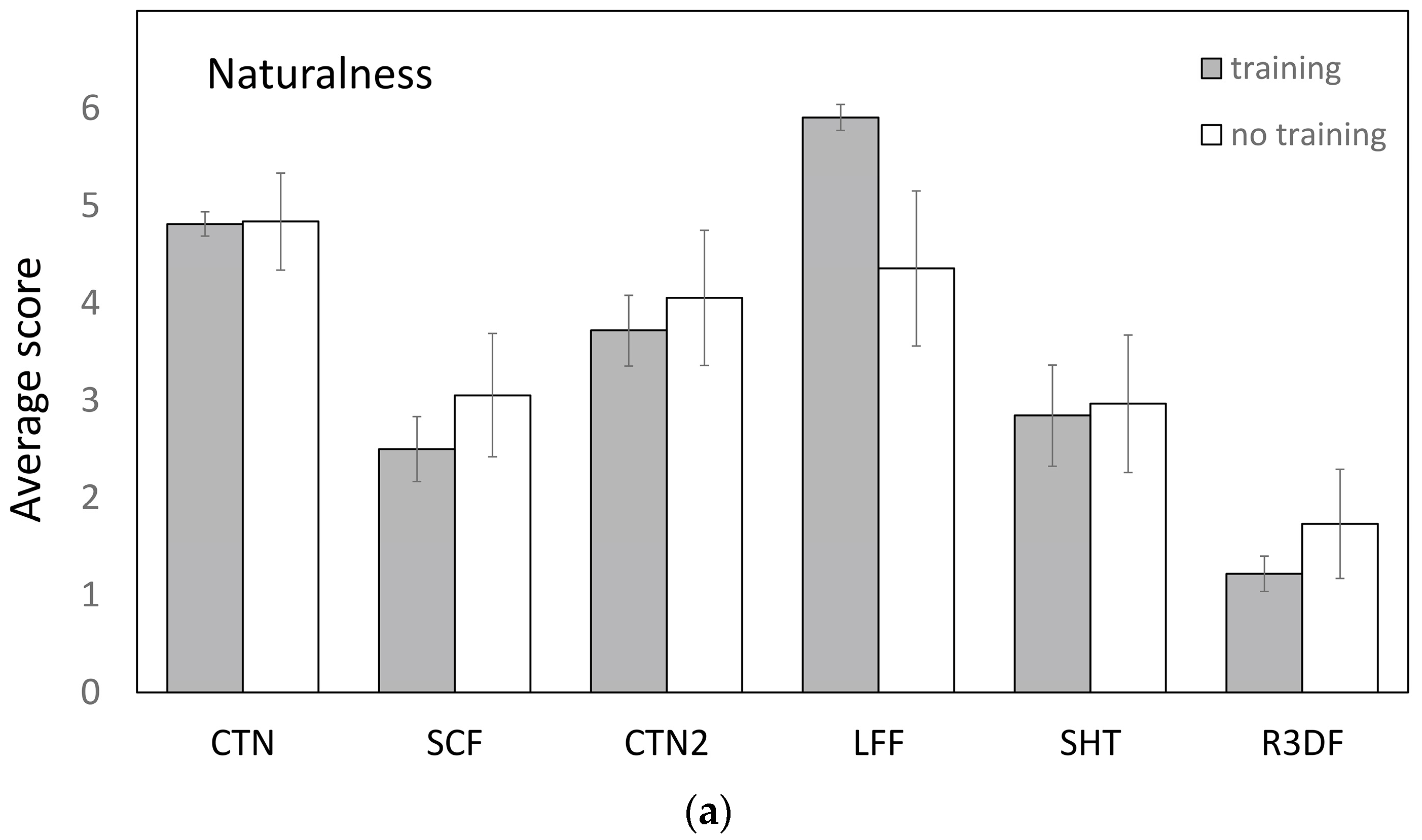
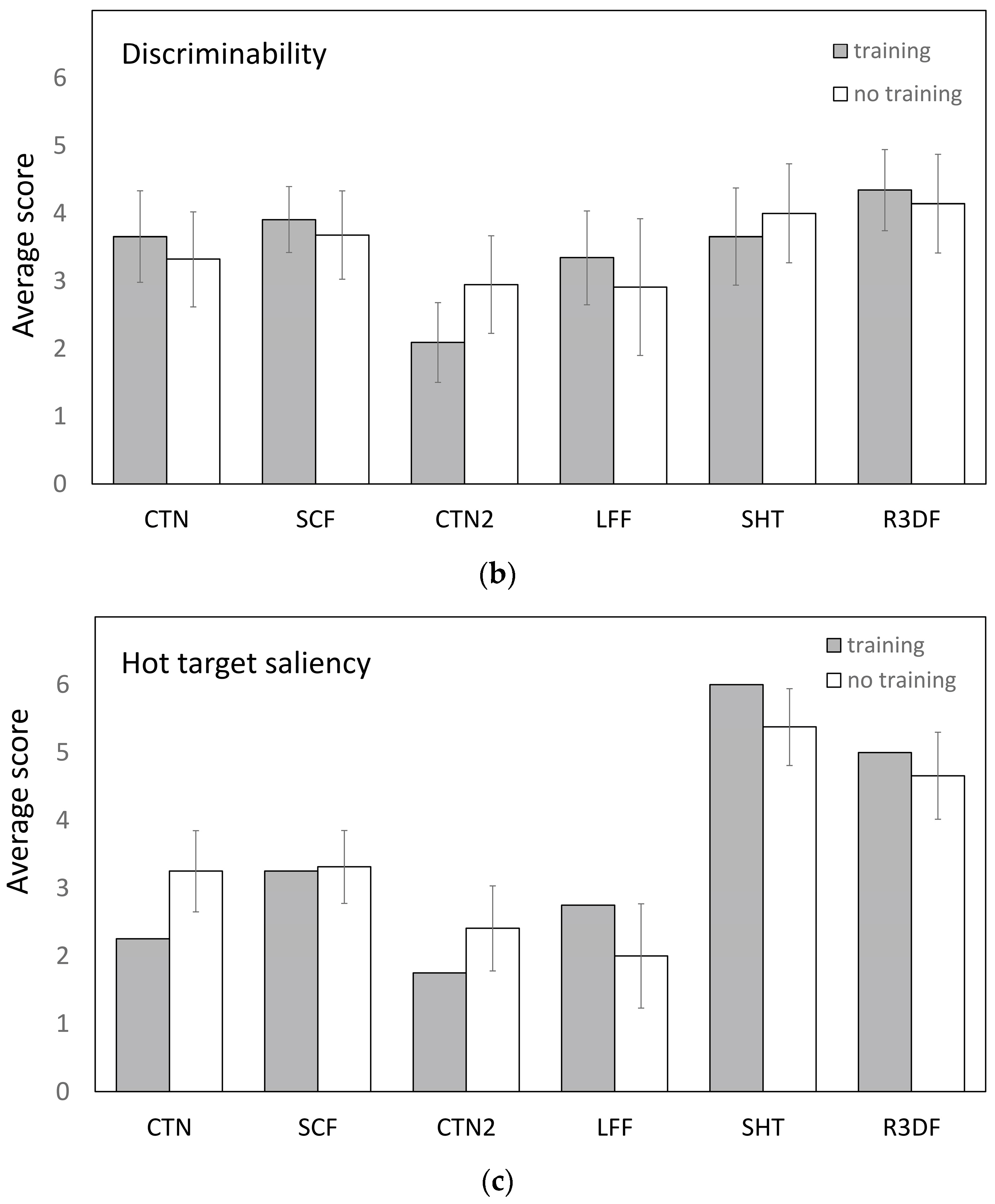
5.1.2. Results

Figure 17 shows the mean observer ranking scores for naturalness, discriminability, and hot target saliency for each of the six color fusion methods tested (CTN, SCF, CTN2, LFF, SHT, and R3DF). This figure shows the scores separately both for images that were included and excluded from the training sets.

To measure the inter-rater agreement (also called inter-rater reliability or IRR) between our observers we computed Krippendorff’s alpha, using the R package ‘irr’ [77]. The IRR analysis showed that the observers had a substantial agreement in their ratings on naturalness (α = 0.51), and a very high agreement in their ratings of the Saliency of hot targets in the scenes (α = 0.95). However, they did not agree in their ratings of the discriminability of different materials in the scene (α = 0.03).

Figure 17a shows that the CTN and LFF methods score relatively high on naturalness, while the results of the R3DF method were rated as least natural by the observers. This figure also shows that the LFF method yields more natural looking results especially for images that were included in the training set. For scenes that were not included in the training set the naturalness decreases, meaning that the relation between daytime reference colors and nighttime sensor values does not extrapolate very well to different scenes.

Figure 17b shows that the ratings on discriminability vary largely between observers, resulting in a low inter rater agreement. This may be a result of the fact that different observers used different details in the scene to make their judgments. In a debriefing, some observers remarked that they had paid more attention to the distinctness of vegetation, while others stated that they had fixated more on details of buildings. On average, the highest discriminability scores are given to the R3DF, SHT and SCF color fusion methods (in descending order).

Figure 17c shows that the SHT method, which was specifically designed to enhance the saliency of hot targets in a scene, appears to perform well in this respect. The R3DF method also appears to represent the hot targets at high contrast.

5.2. Objective Quality Metrics

5.2.1. Methods

We used three no-reference and three full-reference computational image quality metrics to objectively assess and compare the performance of the six different color fusion schemes discussed in this study.

The first no-reference metric is the global color image contrast metric (ICM) that measures the global image contrast [78]. The ICM computes a weighted estimate of the dynamic ranges of both the graylevel and color luminance (L* in CIELAB L*a*b* color space) histograms. The range of ICM is [0,1]. Larger ICM values correspond to higher perceived image contrast.

The second no-reference metric is the color colorfulness metric (CCM) that measures the color vividness of an image as a weighted combination of color saturation and color variety [78]. Larger CCM values correspond to more colorful images.

The third no-reference metric is the number of characteristic colors in an image (NC). We obtained this number by converting the RGB images to indexed images using minimum variance quantization [79] with an upper bound of 65,536 possible colors. NC is then the number of colors that are actually used for the indexed image representation.

The first full-reference metric is the color image feature similarity metric (FSIMc) that combines measures of local image structure (computed from phase congruency) and local image contrast (computed as the gradient magnitude) in YIQ color space to measure the degree of correspondence between a color fused image and a daylight reference color image [80]. The range of FSIMc is [0,1]. The larger the FSIMc value of a colorized image is, the more similar it is to the reference image. Extensive evaluation studies on several color image quality databases have shown that FSIMc predicts human visual quality scores for color images [80].

The second full-reference metric is the color natural metric (CNM: [78,81,82]). The CNM measures the similarity of the color distributions of a color fused image and a daylight reference color image in Lab color space using Ma’s [83] gray relational coefficients. The range of CNM is [0,1]. The larger the CNM value of a colorized image is, the more similar its color distribution is to that of the reference image.

The third full-reference metric is the objective evaluation index (OEI: [81,82]). The OEI measures the degree of correspondence between a color fused image and a daylight reference color image by effectively integrating four established image quality metrics in CIELAB L*a*b* color space: phase congruency (representing local image structure; [84]), gradient magnitude (measuring local image contrast or sharpness), image contrast (ICM), and color naturalness (CNM). The range of OEI is [0,1]. The larger the OEI value of a colorized image is, the more similar it is to the reference image.

5.2.2. Results

Table 1. Results of the computational image quality metrics (with their standard error) for each of the color fusion methods investigated in this study. Overall highest values are printed in bold.

Method	No-Reference Metric			Full-Reference Metric
	ICM	CCM	NC	FSIMc	CNM	OEI
CTN	0.382 (0.008)	4.6 (1.2)	815 (43)	0.78 (0.02)	0.82 (0.02)	0.73 (0.02)
SCF	0.370 (0.006)	3.6 (1.0)	1589 (117)	0.77 (0.02)	0.76 (0.02)	0.72 (0.02)
CTN2	0.380 (0.008)	4.4 (1.2)	938 (102)	0.78 (0.02)	0.82 (0.02)	0.73 (0.02)
LFF	0.358 (0.009)	4.5 (1.2)	860 (64)	0.80 (0.01)	0.82 (0.02)	0.74 (0.02)
SHT	0.349 (0.007)	4.4 (1.2)	1247 (241)	0.78 (0.01)	0.82 (0.02)	0.72 (0.02)
R3DF	0.341 (0.011)	4.1 (1.1)	2630 (170)	0.77 (0.01)	0.74 (0.02)	0.70 (0.03)

ICM = image contrast metric, CCM = color colorfulness metric, NC = number of colors, FSIMc = feature similarity metric, CNM = color natural metric, OEI = objective evaluation index.

shows the mean values (with their standard error) of the computational image metrics for each of the six color fusion methods investigated in this study. The full-reference FSIMc, CNM and OEI metrics all assign the largest values to the LFF method. This result agrees with our subjective observation that LFF produces color fused imagery with the most natural appearance (Section 5.1.2). The original CTN method also appears to perform well overall, with the highest mean image contrast (ICM), image colorfulness (CCM) and color naturalness (CNM) values. In addition, the sample-based CTN method outperforms the statistical SCF method (which is computationally more expensive and yields a less stable color representation) on all quality metrics. The low CNM value for the R3DF method confirms our subjective observation that the imagery produced by this method yields looks less natural. CTN and CTN2 both have the same CNM values, and do not differ much in their CCM values, supporting our qualitative and somewhat surprising observation that CTN2 does not lead to more naturalistic colors than the three band CTN color mapping.

To assess the overall agreement between the observer judgements and the computational metrics we computed Spearman’s rank correlation coefficient between all six computational image quality metrics and the observer scores for naturalness, discriminability and saliency of hot targets (

Table 2. Pearson’s correlation coefficient between the computational image quality metrics and the observer ratings for naturalness, discriminability and the saliency of hot targets. Overall highest values are printed in bold.

Method	No-Reference Metric			Full-Reference Metric
	ICM	CCM	NC	FSIMc	CNM	OEI
Naturalness	0.66	0.64	0.92	0.81	0.81	0.95
Discriminability	0.68	0.45	0.77	0.67	0.66	0.84
Saliency hot targets	0.68	0.16	0.58	0.65	0.32	0.77

). Most computational metrics show a significant correlation with the human observer ratings for naturalness. It appears that the OEI metric most strongly predicts the human observer ratings on all three criteria. This agrees with a previous finding in the literature that the OEI metric ranked different color fused images similar as human observers [81]. The correlation between the OEI and perceived naturalness is specially high (0.95).

6. Discussion and Conclusions

We have proposed three new methods that focus on improving performance in different military tasks. The luminance-fit (LFF) method was intended to give a result in which the luminance more closely matches the daytime situation (compared to the result of the CTN method). Both our qualitative and quantitative (observer experiments and computational image quality metrics) evaluations indicate that this is indeed the case. This method is especially suited for situations in which natural daytime colors are required (leading to good situational awareness, and fast and easy interpretation) and for systems that need to be operated by untrained users. The disadvantage of this method over the CTN-scheme is that it leads to a somewhat lower discriminability of different materials. Again, the choice between the two fusion schemes has to be based on the application (i.e., adapted to the task and situation).

Secondly, we proposed a salient-hot-targets (SHT) fusion scheme, intended to render hot targets as more salient by painting the hot elements in more vibrant colors. The results of the quantitative evaluation tests show that this method does indeed represent hot elements as more salient in the fused image in most situations. However, in some cases a decrease in saliency may result. This suggests that this fusion scheme may be improved, e.g., by adapting the luminance of the hot elements to that of their local background (i.e., by enhancing local luminance contrast), or by using a different mixing scheme (e.g., by replacing the scheme depicted in the inset of Figure 10b by a different one).

Our third proposal was to create a color fusion method (rigid-3D-fit or R3DF method) that combines the advantages of the sample-based method (the fact that the direct correspondence between sensor values and output colors is used to create a result that closely matches the daytime image) along with the advantages of the statistical method (the fact that this method leads to a smooth transformation in which a fuller range of colors is used, leading to better discriminability of materials). A rigid-3D-fit was used to transform the input (sensor values) and output (daytime colors) (by mapping their CLUTs) to assure that the color space did not collapse under the transformation. The results of this fusion scheme look somewhat similar to that of the statistical method, although the colors are somewhat less naturalistic (but still intuitive). However, this method results in better discriminability of materials and has good generalization properties (i.e., it transfers well to untrained scenes). This is probably due to the fact that the transformation is constrained by the direct correspondence between input and output (and not only by the widths of the distributions). This fusion method is especially suited for applications in which the discriminability of different materials is important while the exact color is somewhat less important. Still, the colors that are generated are quite intuitive. Another advantage of this method is that the transformation may be derived from a very limited number of image samples (e.g., N = 4), and does not rely on a large training set spanning the complete set of possible multiband sensor values. The transformation can be made to yield predefined colors for elements of interest in the scene (e.g., vegetation, certain targets).

The results from both our qualitative and quantitative evaluation studies show that the original CTN method works quite well and that it shows good transfer to untrained imagery taken in the same environment and with similar sensor settings. Even in cases in which the environment or sensor settings are different, it still applies reasonably well.

Surprisingly, the CTN2 two-band mapping does not performs as well as expected, even when applied to untrained scenes. This suggests that there may be a relationship between the daytime colors and the LWIR sensor values which the fusion method utilizes and that this also applies to the untrained situations. It may be the case that there are different types of environments in which this relationship differs and that we happen to have recorded (and evaluated) environments in which this relationship was quite similar. Given the limited dataset we used (and which is freely available for research purposes: [74]) this may not be surprising. It suggests that the system should be trained with scenes representing different types of environments in which LWIR can be used to infer the daytime color.

One of the reasons why the learned color transformation does not always transfer well to untrained situations is probably that, in a new situation, the sensor settings can differ considerably. When, for instance, the light level changes, the (auto)gain settings may change, and one may end up in a very different location in 3D sensor/color space, which may ultimately result in very different output colors (for the same object). This can be only be prevented by using the sensor settings to recalculate (recalibrate) the values to those that would have been obtained if sensor settings had been used that corresponded to the training situation.

The set of images that is available for testing is still rather limited. Therefore, we intend to extend our dataset to include more variation in backgrounds, environmental conditions (weather, light conditions, etc.), which can serve as a benchmark set for improving and testing new color fusion schemes in the future.

References

- Li, S.; Kang, X.; Fang, L.; Hu, J.; Yin, H. Pixel-level image fusion: A survey of the state of the art. Inf. Fusion 2017, 33, 100–112. [Google Scholar] [CrossRef]
- Mahmood, S.; Khan, Y.D.; Khalid Mahmood, M. A treatise to vision enhancement and color fusion techniques in night vision devices. Multimed. Tools Appl. 2017, 76, 1–49. [Google Scholar] [CrossRef]
- Zheng, Y. An Overview of Night Vision Colorization Techniques Using Multispectral Images: From Color Fusion to Color Mapping. In Proceedings of the IEEE International Conference on Audio, Language and Image Processing (ICALIP), Shanghai, China, 16–18 July 2012; pp. 134–143. [Google Scholar]
- Toet, A.; Hogervorst, M.A. Progress in color night vision. Opt. Eng. 2012, 51, 010901. [Google Scholar] [CrossRef]
- Zheng, Y. An exploration of color fusion with multispectral images for night vision enhancement. In Image Fusion and Its Applications; Zheng, Y., Ed.; InTech Open: Rijeka, Croatia, 2011; pp. 35–54. [Google Scholar]
- Wichmann, F.A.; Sharpe, L.T.; Gegenfurtner, K.R. The contributions of color to recognition memory for natural scenes. J. Exp. Psychol. Learn. Mem. Cognit. 2002, 28, 509–520. [Google Scholar] [CrossRef]
- Bramão, I.; Reis, A.; Petersson, K.M.; Faísca, L. The role of color information on object recognition: A review and meta-analysis. Acta Psychol. 2011, 138, 244–253. [Google Scholar] [CrossRef] [PubMed]
- Sampson, M.T. An Assessment of the Impact of Fused Monochrome and Fused Color Night Vision Displays on Reaction Time and Accuracy in Target Detection; Report AD-A321226; Naval Postgraduate School: Monterey, CA, USA, 1996. [Google Scholar]
- Gegenfurtner, K.R.; Rieger, J. Sensory and cognitive contributions of color to the recognition of natural scenes. Curr. Biol. 2000, 10, 805–808. [Google Scholar] [CrossRef]
- Tanaka, J.W.; Presnell, L.M. Color diagnosticity in object recognition. Percept. Psychophys. 1999, 61, 1140–1153. [Google Scholar] [CrossRef] [PubMed]
- Castelhano, M.S.; Henderson, J.M. The influence of color on the perception of scene gist. J. Exp. Psychol. Hum. Percept. Perform. 2008, 34, 660–675. [Google Scholar] [CrossRef] [PubMed]
- Rousselet, G.A.; Joubert, O.R.; Fabre-Thorpe, M. How long to get the “gist” of real-world natural scenes? Vis. Cognit. 2005, 12, 852–877. [Google Scholar] [CrossRef]
- Goffaux, V.; Jacques, C.; Mouraux, A.; Oliva, A.; Schyns, P.; Rossion, B. Diagnostic colours contribute to the early stages of scene categorization: Behavioural and neurophysiological evidence. Vis. Cognit. 2005, 12, 878–892. [Google Scholar] [CrossRef]
- Oliva, A.; Schyns, P.G. Diagnostic colors mediate scene recognition. Cognit. Psychol. 2000, 41, 176–210. [Google Scholar] [CrossRef] [PubMed]
- Frey, H.-P.; Honey, C.; König, P. What’s color got to do with it? The influence of color on visual attention in different categories. J. Vis. 2008, 8, 6. [Google Scholar] [CrossRef] [PubMed]
- Bramão, I.; Inácio, F.; Faísca, L.; Reis, A.; Petersson, K.M. The influence of color information on the recognition of color diagnostic and noncolor diagnostic objects. J. Gen. Psychol. 2011, 138, 49–65. [Google Scholar] [CrossRef] [PubMed]
- Spence, I.; Wong, P.; Rusan, M.; Rastegar, N. How color enhances visual memory for natural scenes. Psychol. Sci. 2006, 17, 1–6. [Google Scholar] [CrossRef] [PubMed]
- Ansorge, U.; Horstmann, G.; Carbone, E. Top-down contingent capture by color: Evidence from RT distribution analyses in a manual choice reaction task. Acta Psychol. 2005, 120, 243–266. [Google Scholar] [CrossRef] [PubMed]
- Green, B.F.; Anderson, L.K. Colour coding in a visual search task. J. Exp. Psychol. 1956, 51, 19–24. [Google Scholar] [CrossRef] [PubMed]
- Folk, C.L.; Remington, R. Selectivity in distraction by irrelevant featural singletons: Evidence for two forms of attentional capture. J. Exp. Psychol. Hum. Percept. Perform. 1998, 24, 847–858. [Google Scholar] [CrossRef] [PubMed]
- Driggers, R.G.; Krapels, K.A.; Vollmerhausen, R.H.; Warren, P.R.; Scribner, D.A.; Howard, J.G.; Tsou, B.H.; Krebs, W.K. Target detection threshold in noisy color imagery. In Infrared Imaging Systems: Design, Analysis, Modeling, and Testing XII; Holst, G.C., Ed.; The International Society for Optical Engineering: Bellingham, WA, USA, 2001; Volume 4372, pp. 162–169. [Google Scholar]
- Horn, S.; Campbell, J.; O’Neill, J.; Driggers, R.G.; Reago, D.; Waterman, J.; Scribner, D.; Warren, P.; Omaggio, J. Monolithic multispectral FPA. In International Military Sensing Symposium; NATO RTO: Paris, France, 2002; pp. 1–18. [Google Scholar]
- Lanir, J.; Maltz, M.; Rotman, S.R. Comparing multispectral image fusion methods for a target detection task. Opt. Eng. 2007, 46, 1–8. [Google Scholar] [CrossRef]
- Martinsen, G.L.; Hosket, J.S.; Pinkus, A.R. Correlating military operators’ visual demands with multi-spectral image fusion. In Signal Processing, Sensor Fusion, and Target Recognition XVII; Kadar, I., Ed.; The International Society for Optical Engineering: Bellingham, WA, USA, 2008; Volume 6968, pp. 1–7. [Google Scholar]
- Jacobson, N.P.; Gupta, M.R. Design goals and solutions for display of hyperspectral images. IEEE Trans. Geosci. Remote Sens. 2005, 43, 2684–2692. [Google Scholar] [CrossRef]
- Joseph, J.E.; Proffitt, D.R. Semantic versus perceptual influences of color in object recognition. J. Exp. Psychol. Learn. Mem. Cognit. 1996, 22, 407–429. [Google Scholar] [CrossRef]
- Fredembach, C.; Süsstrunk, S. Colouring the near-infrared. In IS&T/SID 16th Color Imaging Conference; The Society for Imaging Science and Technology: Springfield, VA, USA, 2008; pp. 176–182. [Google Scholar]
- Krebs, W.K.; Sinai, M.J. Psychophysical assessments of image-sensor fused imagery. Hum. Factors 2002, 44, 257–271. [Google Scholar] [CrossRef] [PubMed]
- McCarley, J.S.; Krebs, W.K. Visibility of road hazards in thermal, visible, and sensor-fused night-time imagery. Appl. Ergon. 2000, 31, 523–530. [Google Scholar] [CrossRef]
- Toet, A.; IJspeert, J.K. Perceptual evaluation of different image fusion schemes. In Signal Processing, Sensor Fusion, and Target Recognition X; Kadar, I., Ed.; The International Society for Optical Engineering: Bellingham, WA, USA, 2001; Volume 4380, pp. 436–441. [Google Scholar]
- Toet, A.; IJspeert, J.K.; Waxman, A.M.; Aguilar, M. Fusion of visible and thermal imagery improves situational awareness. In Enhanced and Synthetic Vision 1997; Verly, J.G., Ed.; International Society for Optical Engineering: Bellingham, WA, USA, 1997; Volume 3088, pp. 177–188. [Google Scholar]
- Essock, E.A.; Sinai, M.J.; McCarley, J.S.; Krebs, W.K.; DeFord, J.K. Perceptual ability with real-world nighttime scenes: Image-intensified, infrared, and fused-color imagery. Hum. Factors 1999, 41, 438–452. [Google Scholar] [CrossRef] [PubMed]
- Essock, E.A.; Sinai, M.J.; DeFord, J.K.; Hansen, B.C.; Srinivasan, N. Human perceptual performance with nonliteral imagery: Region recognition and texture-based segmentation. J. Exp. Psychol. Appl. 2004, 10, 97–110. [Google Scholar] [CrossRef] [PubMed]
- Gu, X.; Sun, S.; Fang, J. Coloring night vision imagery for depth perception. Chin. Opt. Lett. 2009, 7, 396–399. [Google Scholar]
- Vargo, J.T. Evaluation of Operator Performance Using True Color and Artificial Color in Natural Scene Perception; Report AD-A363036; Naval Postgraduate School: Monterey, CA, USA, 1999. [Google Scholar]
- Krebs, W.K.; Scribner, D.A.; Miller, G.M.; Ogawa, J.S.; Schuler, J. Beyond third generation: A sensor-fusion targeting FLIR pod for the F/A-18. In Sensor Fusion: Architectures, Algorithms, and Applications II; Dasarathy, B.V., Ed.; International Society for Optical Engineering: Bellingham, WA, USA, 1998; Volume 3376, pp. 129–140. [Google Scholar]
- Scribner, D.; Warren, P.; Schuler, J. Extending Color Vision Methods to Bands Beyond the Visible. In Proceedings of the IEEE Workshop on Computer Vision Beyond the Visible Spectrum: Methods and Applications, Fort Collins, CO, USA, 22 June 1999; pp. 33–40. [Google Scholar]
- Sun, S.; Jing, Z.; Li, Z.; Liu, G. Color fusion of SAR and FLIR images using a natural color transfer technique. Chin. Opt. Lett. 2005, 3, 202–204. [Google Scholar]
- Tsagaris, V.; Anastassopoulos, V. Fusion of visible and infrared imagery for night color vision. Displays 2005, 26, 191–196. [Google Scholar] [CrossRef]
- Zheng, Y.; Hansen, B.C.; Haun, A.M.; Essock, E.A. Coloring night-vision imagery with statistical properties of natural colors by using image segmentation and histogram matching. In Color Imaging X: Processing, Hardcopy and Applications; Eschbach, R., Marcu, G.G., Eds.; The International Society for Optical Engineering: Bellingham, WA, USA, 2005; Volume 5667, pp. 107–117. [Google Scholar]
- Toet, A. Natural colour mapping for multiband nightvision imagery. Inf. Fusion 2003, 4, 155–166. [Google Scholar] [CrossRef]
- Wang, L.; Jin, W.; Gao, Z.; Liu, G. Color fusion schemes for low-light CCD and infrared images of different properties. In Electronic Imaging and Multimedia Technology III; Zhou, L., Li, C.-S., Suzuki, Y., Eds.; The International Society for Optical Engineering: Bellingham, WA, USA, 2002; Volume 4925, pp. 459–466. [Google Scholar]
- Li, J.; Pan, Q.; Yang, T.; Cheng, Y.-M. Color Based Grayscale-Fused Image Enhancement Algorithm for Video Surveillance. In Proceedings of the IEEE Third International Conference on Image and Graphics (ICIG’04), Hong Kong, China, 18–20 December 2004; pp. 47–50. [Google Scholar]
- Howard, J.G.; Warren, P.; Klien, R.; Schuler, J.; Satyshur, M.; Scribner, D.; Kruer, M.R. Real-time color fusion of E/O sensors with PC-based COTS hardware. In Targets and Backgrounds VI: Characterization, Visualization, and the Detection Process; Watkins, W.R., Clement, D., Reynolds, W.R., Eds.; The International Society for Optical Engineering: Bellingham, WA, USA, 2000; Volume 4029, pp. 41–48. [Google Scholar]
- Scribner, D.; Schuler, J.M.; Warren, P.; Klein, R.; Howard, J.G. Sensor and Image Fusion; Driggers, R.G., Ed.; Marcel Dekker Inc.: New York, NY, USA; pp. 2577–2582.
- Schuler, J.; Howard, J.G.; Warren, P.; Scribner, D.A.; Klien, R.; Satyshur, M.; Kruer, M.R. Multiband E/O color fusion with consideration of noise and registration. In Targets and Backgrounds VI: Characterization, Visualization, and the Detection Process; Watkins, W.R., Clement, D., Reynolds, W.R., Eds.; The International Society for Optical Engineering: Bellingham, WA, USA, 2000; Volume 4029, pp. 32–40. [Google Scholar]
- Waxman, A.M.; Gove, A.N.; Fay, D.A.; Racamoto, J.P.; Carrick, J.E.; Seibert, M.C.; Savoye, E.D. Color night vision: Opponent processing in the fusion of visible and IR imagery. Neural Netw. 1997, 10, 1–6. [Google Scholar] [CrossRef]
- Waxman, A.M.; Fay, D.A.; Gove, A.N.; Seibert, M.C.; Racamato, J.P.; Carrick, J.E.; Savoye, E.D. Color night vision: Fusion of intensified visible and thermal IR imagery. In Synthetic Vision for Vehicle Guidance and Control; Verly, J.G., Ed.; The International Society for Optical Engineering: Bellingham, WA, USA, 1995; Volume 2463, pp. 58–68. [Google Scholar]
- Warren, P.; Howard, J.G.; Waterman, J.; Scribner, D.A.; Schuler, J. Real-Time, PC-Based Color Fusion Displays; Report A073093; Naval Research Lab: Washington, DC, USA, 1999. [Google Scholar]
- Fay, D.A.; Waxman, A.M.; Aguilar, M.; Ireland, D.B.; Racamato, J.P.; Ross, W.D.; Streilein, W.; Braun, M.I. Fusion of multi-sensor imagery for night vision: Color visualization, target learning and search. In Third International Conference on Information Fusion, Vol. I-TuD3; IEEE Press: Piscataway, NJ, USA, 2000; pp. 3–10. [Google Scholar]
- Aguilar, M.; Fay, D.A.; Ross, W.D.; Waxman, A.M.; Ireland, D.B.; Racamoto, J.P. Real-time fusion of low-light CCD and uncooled IR imagery for color night vision. In Enhanced and Synthetic Vision 1998; Verly, J.G., Ed.; The International Society for Optical Engineering: Bellinggam, WA, USA, 1998; Volume 3364, pp. 124–135. [Google Scholar]
- Waxman, A.M.; Aguilar, M.; Baxter, R.A.; Fay, D.A.; Ireland, D.B.; Racamoto, J.P.; Ross, W.D. Opponent-Color Fusion of Multi-Sensor Imagery: Visible, IR and SAR. Available online: http://www.dtic.mil/docs/citations/ADA400557 (accessed on 28 August 2017).
- Aguilar, M.; Fay, D.A.; Ireland, D.B.; Racamoto, J.P.; Ross, W.D.; Waxman, A.M. Field evaluations of dual-band fusion for color night vision. In Enhanced and Synthetic Vision 1999; Verly, J.G., Ed.; The International Society for Optical Engineering: Bellingham, WA, USA, 1999; Volume 3691, pp. 168–175. [Google Scholar]
- Fay, D.A.; Waxman, A.M.; Aguilar, M.; Ireland, D.B.; Racamato, J.P.; Ross, W.D.; Streilein, W.; Braun, M.I. Fusion of 2-/3-/4-sensor imagery for visualization, target learning, and search. In Enhanced and Synthetic Vision 2000; Verly, J.G., Ed.; SPIE—The International Society for Optical Engineering: Bellingham, WA, USA, 2000; Volume 4023, pp. 106–115. [Google Scholar]
- Huang, G.; Ni, G.; Zhang, B. Visual and infrared dual-band false color image fusion method motivated by Land’s experiment. Opt. Eng. 2007, 46, 1–10. [Google Scholar] [CrossRef]
- Li, G. Image fusion based on color transfer technique. In Image Fusion and Its Applications; Zheng, Y., Ed.; InTech Open: Rijeka, Croatia, 2011; pp. 55–72. [Google Scholar]
- Zaveri, T.; Zaveri, M.; Makwana, I.; Mehta, H. An Optimized Region-Based Color Transfer Method for Night Vision Application. In Proceedings of the 3rd IEEE International Conference on Signal and Image Processing (ICSIP 2010), Chennai, India, 15–17 December 2010; pp. 96–101. [Google Scholar]
- Zhang, J.; Han, Y.; Chang, B.; Yuan, Y. Region-based fusion for infrared and LLL images. In Image Fusion; Ukimura, O., Ed.; INTECH: Rijeka, Croatia, 2011; pp. 285–302. [Google Scholar]
- Qian, X.; Han, L.; Wang, Y.; Wang, B. Color contrast enhancement for color night vision based on color mapping. Infrared Phys. Technol. 2013, 57, 36–41. [Google Scholar] [CrossRef]
- Li, G.; Xu, S.; Zhao, X. Fast Color-Transfer-Based Image Fusion Method for Merging Infrared and Visible Images; Braun, J.J., Ed.; The International Society for Optical Engineering: Bellingham, WA, USA, 2010; Volume 77100S, pp. 1–12. [Google Scholar]
- Li, G.; Xu, S.; Zhao, X. An efficient color transfer algorithm for recoloring multiband night vision imagery. In Enhanced and Synthetic Vision 2010; Güell, J.J., Bernier, K.L., Eds.; The International Society for Optical Engineering: Bellingham, WA, USA, 2010; Volume 7689, pp. 1–12. [Google Scholar]
- Li, G.; Wang, K. Applying daytime colors to nighttime imagery with an efficient color transfer method. In Enhanced and Synthetic Vision 2007; Verly, J.G., Guell, J.J., Eds.; The International Society for Optical Engineering: Bellingham, WA, USA, 2007; Volume 6559, pp. 1–12. [Google Scholar]
- Shen, H.; Zhou, P. Near natural color polarization imagery fusion approach. In Third International Congress on Image and Signal Processing (CISP 2010); IEEE Press: Piscataway, NJ, USA, 2010; Volume 6, pp. 2802–2805. [Google Scholar]
- Yin, S.; Cao, L.; Ling, Y.; Jin, G. One color contrast enhanced infrared and visible image fusion method. Infrared Phys. Technol. 2010, 53, 146–150. [Google Scholar] [CrossRef]
- Ali, E.A.; Qadir, H.; Kozaitis, S.P. Color night vision system for ground vehicle navigation. In Infrared Technology and Applications XL; Andresen, B.F., Fulop, G.F., Hanson, C.M., Norton, P.R., Eds.; SPIE: Bellingham, WA, USA, 2014; Volume 9070, pp. 1–5. [Google Scholar]
- Jiang, M.; Jin, W.; Zhou, L.; Liu, G. Multiple reference images based on lookup-table color image fusion algorithm. In International Symposium on Computers & Informatics (ISCI 2015); Atlantis Press: Amsterdam, The Netherlands, 2015; pp. 1031–1038. [Google Scholar]
- Sun, S.; Zhao, H. Natural color mapping for FLIR images. In 1st International Congress on Image and Signal Processing CISP 2008; IEEE Press: Piscataway, NJ, USA, 2008; pp. 44–48. [Google Scholar]
- Li, Z.; Jing, Z.; Yang, X. Color transfer based remote sensing image fusion using non-separable wavelet frame transform. Pattern Recognit. Lett. 2005, 26, 2006–2014. [Google Scholar] [CrossRef]
- Hogervorst, M.A.; Toet, A. Fast natural color mapping for night-time imagery. Inf. Fusion 2010, 11, 69–77. [Google Scholar] [CrossRef]
- Hogervorst, M.A.; Toet, A. Presenting Nighttime Imagery in Daytime Colours. In Proceedings of the IEEE 11th International Conference on Information Fusion, Cologne, Germany, 30 June–3 July 2008; pp. 706–713. [Google Scholar]
- Hogervorst, M.A.; Toet, A. Method for applying daytime colors to nighttime imagery in realtime. In Multisensor, Multisource Information Fusion: Architectures, Algorithms, and Applications 2008; Dasarathy, B.V., Ed.; The International Society for Optical Engineering: Bellingham, WA, USA, 2008; pp. 1–9. [Google Scholar]
- Toet, A.; de Jong, M.J.; Hogervorst, M.A.; Hooge, I.T.C. Perceptual evaluation of color transformed multispectral imagery. Opt. Eng. 2014, 53, 043101. [Google Scholar] [CrossRef]
- Toet, A.; Hogervorst, M.A. TRICLOBS portable triband lowlight color observation system. In Multisensor, Multisource Information Fusion: Architectures, Algorithms, and Applications 2009; Dasarathy, B.V., Ed.; The International Society for Optical Engineering: Bellingham, WA, USA, 2009; pp. 1–11. [Google Scholar]
- Toet, A.; Hogervorst, M.A.; Pinkus, A.R. The TRICLOBS Dynamic Multi-Band Image Data Set for the development and evaluation of image fusion methods. PLoS ONE 2016, 11, e0165016. [Google Scholar] [CrossRef] [PubMed]
- Pitié, F.; Kokaram, A.C.; Dahyot, R. Automated colour grading using colour distribution transfer. Comput. Vis. Image Underst. 2007, 107, 123–137. [Google Scholar] [CrossRef]
- Arun, K.S.; Huang, T.S.; Blostein, S.D. Least-squares fitting of two 3-D point sets. IEEE Trans. Pattern Anal. Mach. Intell. 1987, 5, 698–700. [Google Scholar] [CrossRef]
- Gamer, M.; Lemon, J.; Fellows, I.; Sing, P. Package ‘irr’: Various Coefficients of Interrater Reliability and Agreement (Version 0.84). 2015. Available online: http://CRAN.R-project.org/package=irr (accessed on 25 August 2017).
- Yuan, Y.; Zhang, J.; Chang, B.; Han, Y. Objective quality evaluation of visible and infrared color fusion image. Opt. Eng. 2011, 50, 1–11. [Google Scholar] [CrossRef]
- Heckbert, P. Color image quantization for frame buffer display. Comput. Gr. 1982, 16, 297–307. [Google Scholar] [CrossRef]
- Zhang, L.; Zhang, L.; Mou, X.; Zhang, D. FSIM: A feature similarity index for image quality assessment. IEEE Trans. Image Process. 2011, 20, 2378–2386. [Google Scholar] [CrossRef] [PubMed]
- Zheng, Y.; Dong, W.; Chen, G.; Blasch, E.P. The Objective Evaluation Index (OEI) for Evaluation of Night Vision Colorization Techniques; Miao, Q., Ed.; New Advances in Image Fusion; InTech Open: Rijeka, Croatia, 2013; pp. 79–102. [Google Scholar]
- Zheng, Y.; Dong, W.; Blasch, E.P. Qualitative and quantitative comparisons of multispectral night vision colorization techniques. Opt. Eng. 2012, 51, 087004. [Google Scholar] [CrossRef]
- Ma, M.; Tian, H.; Hao, C. New method to quality evaluation for image fusion using gray relational analysis. Opt. Eng. 2005, 44, 1–5. [Google Scholar]
- Kovesi, P. Image features from phase congruency. Videre J. Comput. Vis. Res. 1999, 1, 2–26. [Google Scholar]