1. Introduction
Projectors are used in scientific visualizations, virtual and augmented reality systems, structured light techniques and other visually intensive applications. In the last few years, a number of approaches have been proposed in order to calibrate projectors. As pointed out in Brown et al. [
1], calibration of a projector can be achieved by two different strategies: (1) through mechanical and electronic alignment; (2) by using one or more cameras that observe one or a set of projected images. While the first strategy may be more accurate and easier for the non-expert user, it brings several drawbacks, e.g., the requirement of a special infrastructure and/or resources that can considerably increase the system’s costs. The calibration hardware is no longer needed when the system is calibrated and can be a hindrance. On the contrary, the second approach is less flashy and less time-consuming, although it requires a solid software background. Due to that, several vision-based techniques have been recently proposed to calibrate projectors, some of them being introduced in the following lines.
Many works on projector or multi-projector displays are based on planar surfaces [
2,
3,
4,
5,
6,
7,
8], for which automated geometric correction and alignment is simplified through the use of planar homographies between the planar screen, the projector frame buffers, and the images of one or more cameras observing the screen. Many of these developments use chessboards-based planar references alone or with a combination of other planar surfaces to automatically measure 2D points (i.e., image points) and establish point correspondences [
8,
9,
10,
11,
12,
13,
14]. Other authors use augmented reality markers to establish such correspondences or other kind of self-designed planar markers [
15,
16,
17,
18]. In these developments, usually a physical pattern exists onto where another pattern is projected. The physical pattern is used to compute camera calibration, while the projected pattern is used to compute projector calibration. Some authors use a more complex mathematical background, as the one given in Knyaz [
18], which uses bundle adjustment to derive all unknowns in a single step. As these implementations are based on planar homographies, several views from the reference pattern are needed.
On the other hand, fewer works can be found where non-planar surfaces are used to achieve calibration. In Raskar et al. [
19], projective geometry is used to fully calibrate a camera pair, where a 3D calibration pattern with spatially-known control points (CPs) is used. These points are used to establish 2D-3D correspondences with the related camera image points, and thus compute the projection matrix for each camera. Once both cameras are calibrated, they use the projector to project a grid, on a point-by-point basis. Applying stereo-pair triangulation from the images captured by the 2-camera stereoscopic system, the spatial coordinates of those points are computed, and therefore the projection screen is geometrically defined. Finally, they establish 2D-3D correspondences to fully calibrate the projector in the same way as the cameras.
Other authors make use of structured light techniques. For instance, in Tardif et al. [
20] an approach is presented that allows one or more projectors to display an undistorted image on a surface of unknown geometry. Structured light patterns are used to compute the relative geometries between camera and projector, and thus no explicit calibration is used. In Harville et al. [
21], a method is proposed to project imagery without distortion onto a developable surface—e.g., flat walls, piecewise-planar shapes, cylindrical and conical sections—in such a way that the images to be displayed appear like a wallpaper on the display surface. Camera-projector correspondences are obtained by using a structured light approach that is based on projecting a sequence of bar images (8 to 12 images) of increasingly fine spatial frequency to temporally encode the projector coordinates corresponding to various camera pixels. Since they demonstrate that it is not necessary to obtain the 3D shape of the projection screen, it is only applied to reproduce a wallpaper effect. An improved approach is presented in Sun et al. [
22] by combining the advantages of global surface fitting and homographies to generate high accuracy geometric corrections that are independent of the calibration camera’s location and viewing angle.
A different approach is introduced in Sajadi and Majumder [
23], where spatial geometric relationships are established to derive the exterior orientation of a camera and the interior and exterior orientation of a projector. They use some assumptions, as known interior camera orientation parameters, known shape of the projection screen—which is a vertically extruded cylinder surface—and known aspect ratio of the rectangle formed by the four corners of the screen. A more generic approach is presented in Sajadi and Majumder [
24] for any kind of extruded surfaces.
More recently, Zhao et al. [
25] introduced a two-step approach based on Bézier patches to calibrate projectors on cylindrical surfaces. In the first step, a rough calibration is performed by projecting a total of eight encoded images per projector onto the surface. In a second step, an accurate calibration is performed to correct the errors in the overlap region of adjacent projectors by using the Bézier surface to slightly distort the projected images. In Chen et al. [
26], a method to calibrate a multi-projector light field is presented that consists of transferring the calibration of a 3D scene into the calibration of a 2D image on a diffuser interface, a curved screen. Their setup includes a set of printed and projected points and a precise rotary table where a CCD camera is fixed.
The aim of our research work is to design and deploy a multi-projector calibration method that is not time-consuming and easy-to-use, while relaying on any kind of analytically defined surfaces which can be found in virtual reality simulators. In the scope of the paper, the implemented method is tested and validated with a Formula 1 (F1) virtual reality simulator that has a cylindrical screen and where the image is formed with the conjunction of three projectors. The mathematical background of our approach is based on a combination of surveying, photogrammetry and image processing approaches, and has been designed by considering the geometric restrictions of virtual reality simulators, where the available space is limited and no special infrastructure can be added to calibrate the projectors. Our method combines the simplicity of acquiring in-situ data with inexpensive devices with the simplicity of its mathematical formulation, and thus the procedure can be carried out by non-experienced users.
2. Materials and Methods
2.1. Hardware Components
As introduced above, the designed method has been tested and validated with a F1 virtual reality simulator, whose construction details and characteristics are here explained.
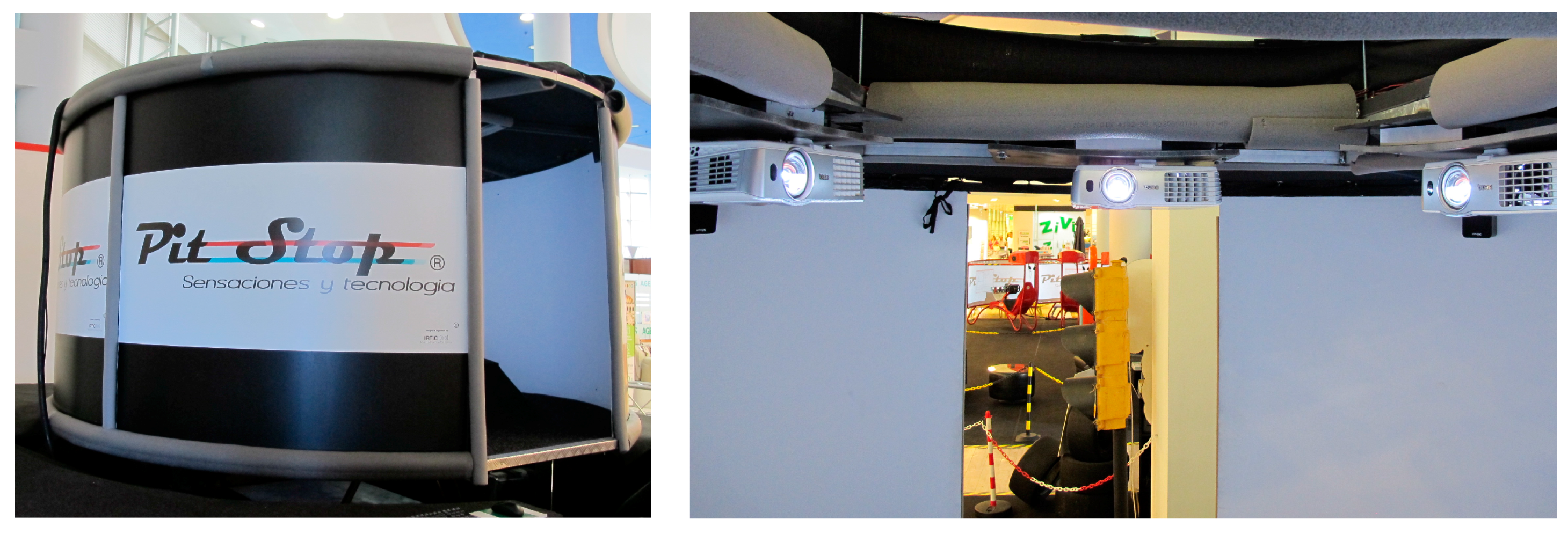
The simulator has been designed and constructed at the Institute of Robotics and Information and Communication Technologies (IRTIC) of the Universitat de València with off-the-shell components (
Figure 1, left). It consists of a motion platform with 6 DoF (Degrees of Freedom), a replica of a F1 pilot seat and a cylindrical surface where virtual contents are projected. The motion platform is able to reproduce accelerations up to 0.8 G with rotational limits of 35° and longitudinal displacements of ±150 mm. It uses the classical washout algorithm [
27], the parameters of which are tuned by a genetic algorithm [
28] to provide a standard setup, valid for most users. The system provides 330° of horizontal FoV (Field of View)—although the current configuration is set-up for 280° and 55° of vertical FoV, where the virtual contents are displayed by the projection of three projectors (
Figure 1, right). Projectors are placed upside-down and they have Full HD resolution each. The total pixel resolution of the system is, thus, 5760 × 1080 pixels.
2.2. Multi-Projector Calibration Method with Analytically Defined Screens
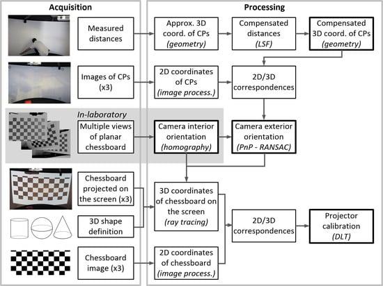
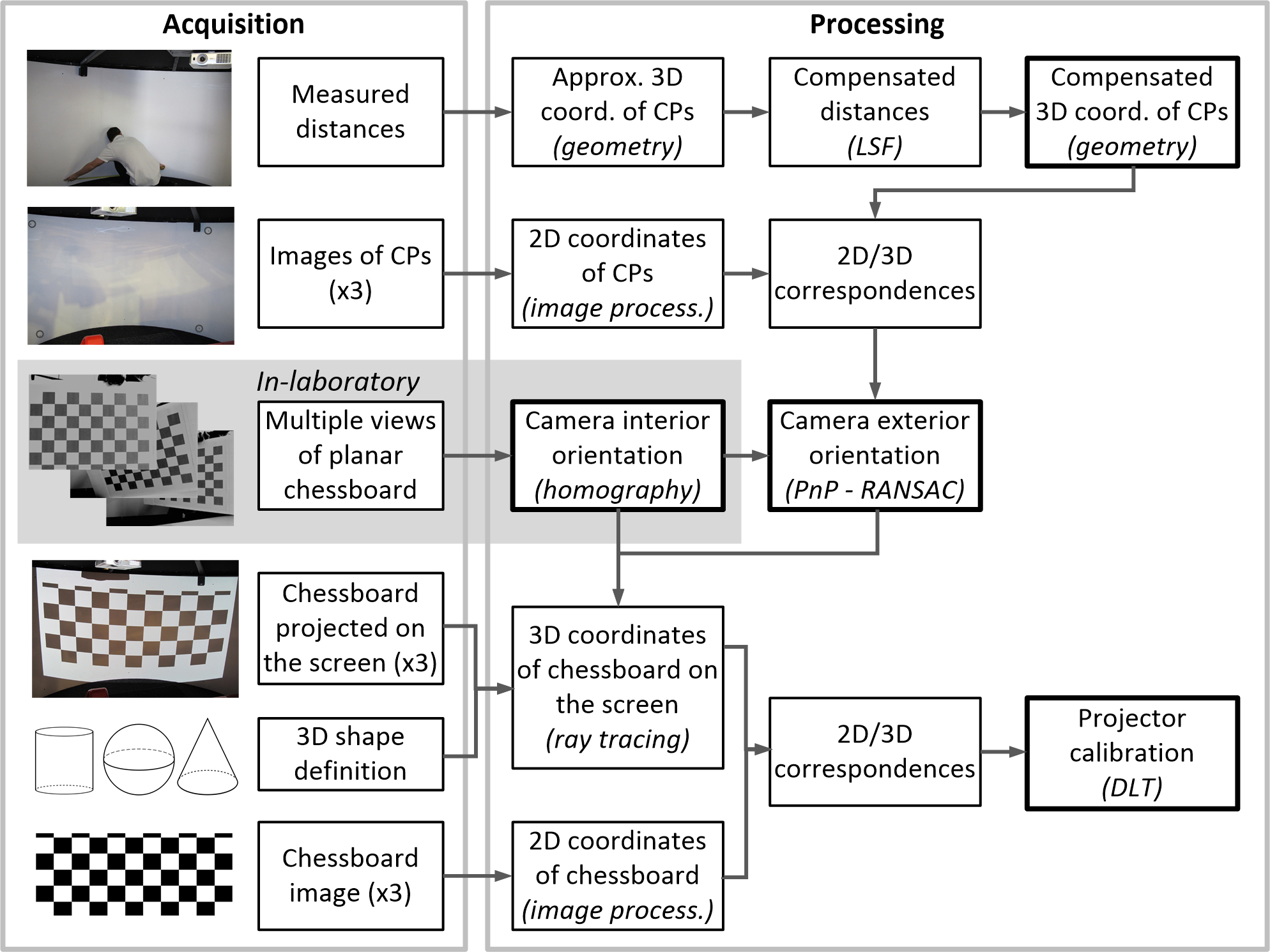
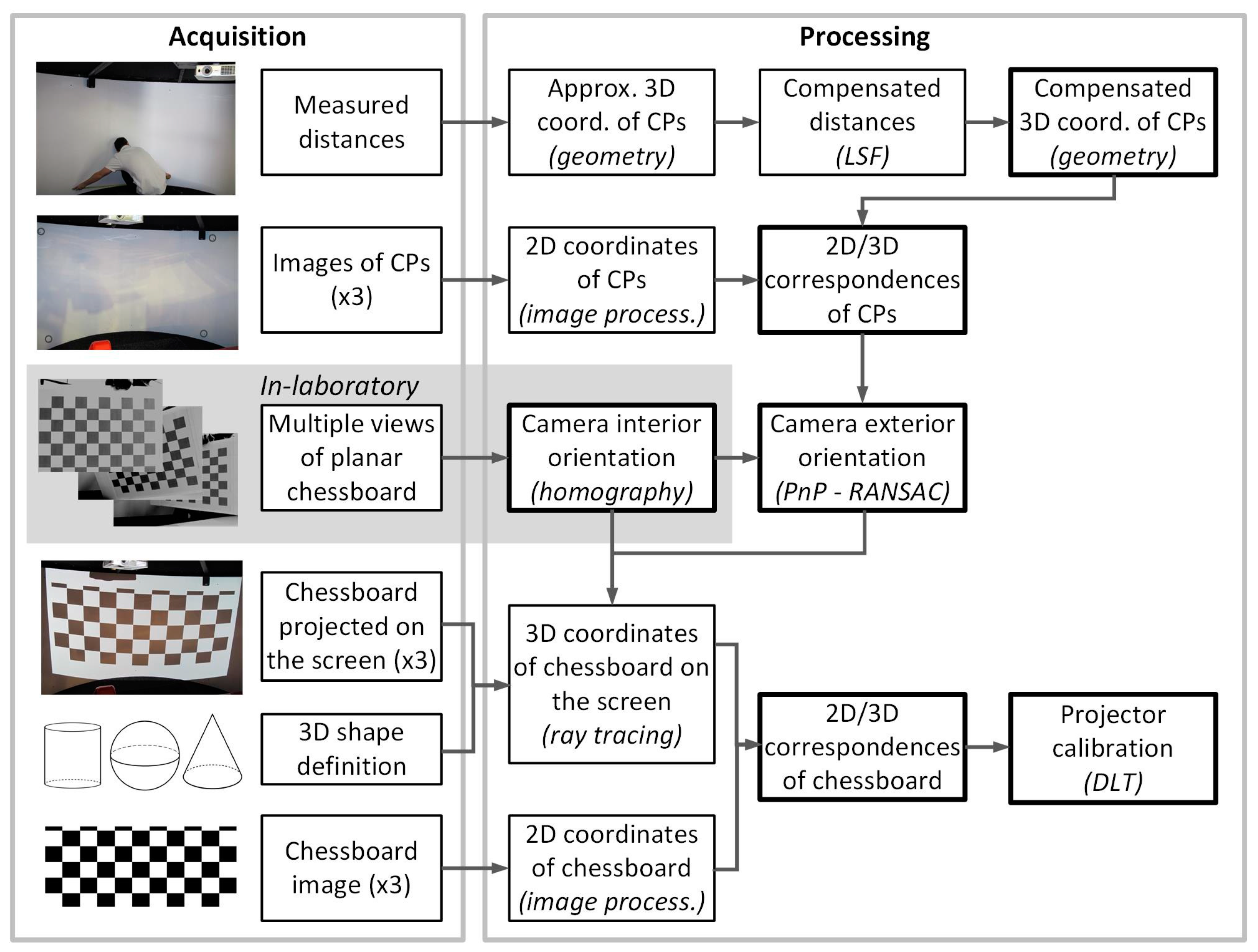
The multi-projector calibration method here proposed involves approaches from surveying, photogrammetry and image processing. A flowchart of the complete methodology is depicted in
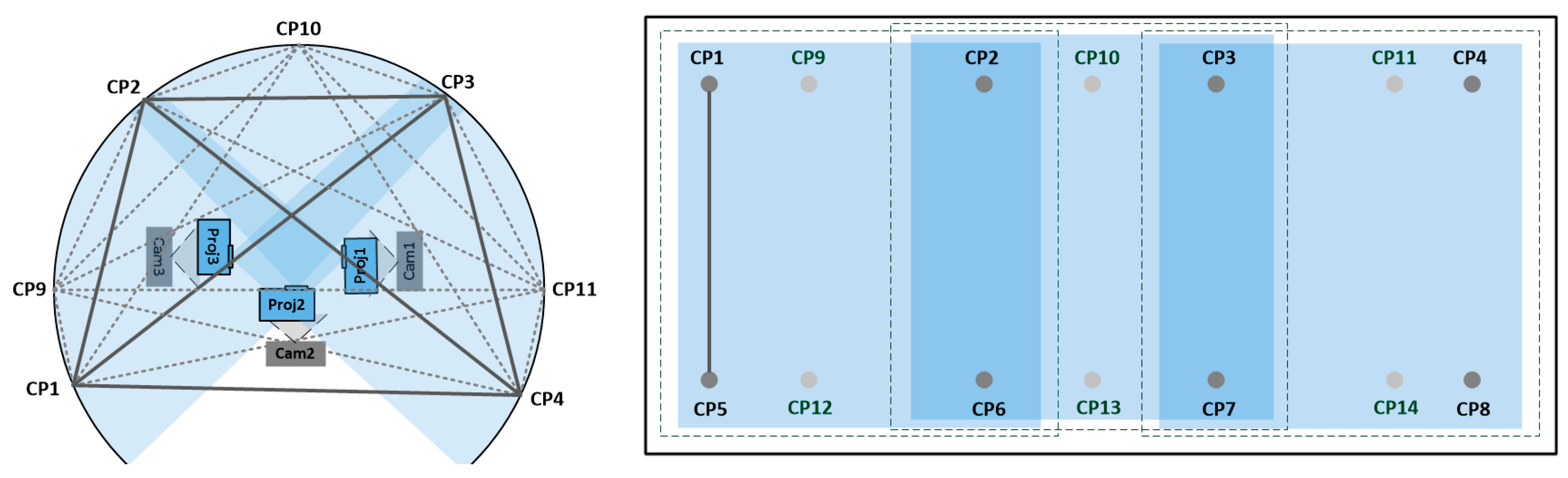
Figure 2, where the main procedures that are explained in the following sub-sections are highlighted. Overall, a single camera is used in order to calibrate the three projectors (Proj1, Proj2 and Proj3 in
Figure 3), which is placed in three different positions (Cam1, Cam2 and Cam3 in
Figure 3). In a first step, the camera interior and exterior orientation parameters have to be calculated, as they are needed to calibrate the projectors. For the external camera calibration, 2D/3D correspondences of a set of Control Points (CPs) are needed, whose object coordinates can be computed from measured distances in the object space. To calibrate the projector, the Direct Linear Transformation (DLT) equations are followed, from which interior and exterior orientation parameters can be derived.
2.2.1. Compensated 3D Coordinates of CPs
Each CP consists of a physical point on the screen. For the sake of simplifying the measuring procedure, the CPs are placed in two rows of vertically aligned pairs, as depicted in
Figure 3 right, for the case of a cylindrical screen, where CPs from 1 to 8 are the minimum number of required CPs (four per camera), while CPs from 9 to 14 are optional but recommendable, with the purpose of having redundancies. A set of distances are measured with a measuring tape to calculate the 3D coordinates of the CPs, from each one of the CPs to the rest in a single row; distances of the second row are considered equal, as CPs are vertically aligned. These distances are depicted in
Figure 3, where continuous lines represent distances from required CPs, and dotted lines represent distances from additional CPs. Additionally, the height between the two rows of vertical CPs, which is constant, is required. This procedure can be done at the laboratory as the cylindrical screen remains with a constant shape. In such a case, the calibration procedure in situ is considerably faster.
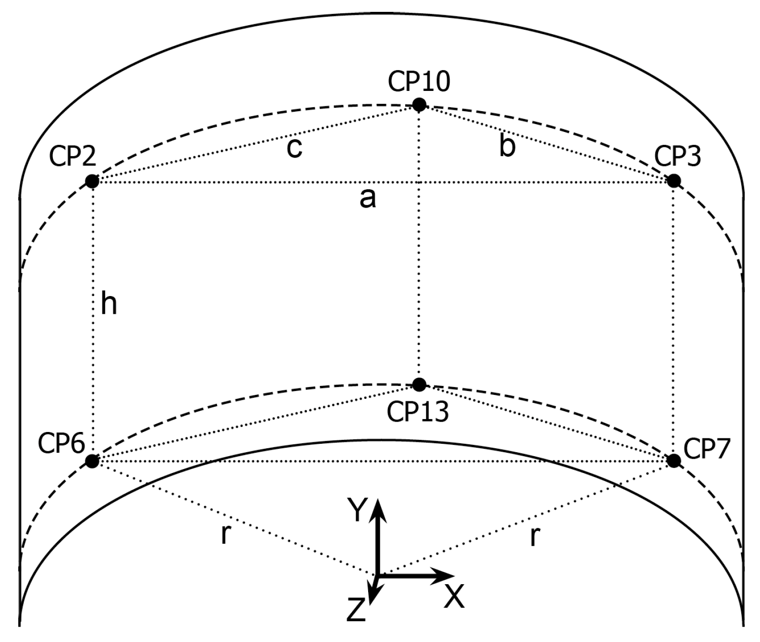
Once we have the measured distances, the 3D coordinates of CPs can be calculated, which will be approximate as the measured distances have not yet been compensated for. In order to derive the 3D coordinates, we establish a coordinate system whose origin is located in the intersection of the horizontal plane defined by the bottom CPs (CP5, CP12, etc.) and the central axes of the cylinder. The coordinate system is vertically aligned in its
Y-axis. The
X-axis is parallel to the direction CP6-CP7, the
Z-axis is perpendicular to the plane defined by the
X-axis and the
Y-axis, and the three axes define a right-handed coordinate system, as depicted in
Figure 4. In such a coordinate system, the 3D approximate coordinates of control points can be derived by applying simple geometrical rules, as indicated in
Table 1, where
,
,
. The radius of the cylinder is also calculated applying simple geometrical rules, from the triangle defined by the distances
a,
b and
c.
Redundant measurements are considered with the purpose of reducing errors in the calculation of CPs after applying a compensation with a Least Squares Fitting (LSF). In that way, errors due to both the limited accuracies of the measuring device (measuring tape) and to the local mechanical distortions introduced during the construction of the cylindrical screen, can be reduced. The mathematical model of LSF is depicted in Equation (1) in the form of indirect observations [
29]. In this equation,
A is the design matrix,
X is the vector of the unknowns,
R is the vector of the residuals and
K is the vector holding the independent factors. The design matrix
A is constructed from the equation shown in (2), which represents the mathematical form of an observed distance. In this equation,
is the approximated calculated value of the distance between
i and
j,
is the differential value of
,
is the approximated calculated azimuth of the distance
and
dzj,
dzi,
dxj and
dxi are the unknowns, which are the corrections to the coordinates
X and
Z of points
j and
i (any pair of CPs). The equation of the azimuth is given in (3). The solution of the unknowns (
dzj,
dzi,
dxj and
dxi) is depicted in Equation (4), which is known as the normal equations. Finally, the
X and
Z compensated coordinates of CPs are calculated as shown in (5) and (6). Note that the
Y coordinates are not compensated in this procedure, as the height
h is directly measured on the screen surface, and thus is acquired with more accuracy.
As an alternative to the measuring process here explained, the CPs could be directly derived with other surveying methods. For instance, a total station could be used instead, that directly derives 3D object coordinates. However, this would require the use of an expensive device and the need of an experienced user to properly collect data. This is precisely one of the issues that we would like to avoid and that motivates the development of our method. Additionally, due to the spatial limitations of most virtual reality simulators, measurements with these devices may not be feasible.
2.2.2. 2D/3D Correspondences of CPs
CPs image coordinates (or 2D coordinates) and the assignment of correspondences is done in a semi-automated manner. In the first place, CPs are automatically extracted from the images acquired by the cameras by detecting black points on the white surface. To that end, the OpenCV library [
30] has been used. The computation of the 2D coordinates with sub-pixel resolution is straightforward with pattern-based image processing techniques available in OpenCV. In order to assign the 2D/3D correspondences, the user has to interactively select the corresponding CP identifiers at each image.
2.2.3. Camera Interior Orientation
To determine the interior orientation camera parameters, an algorithm has been implemented that makes use of the OpenCV library. In this approach the interior orientation procedure is based on the Zhang method [
31] to solve for the focal length and principal point offsets (
c,
x0 and
y0). On the other hand, the tangential and radial distortion coefficients are computed following the method described in [
32]. The equations used in OpenCV for correcting radial distortion are shown in Equations (7) and (8), where
k1,
k2 and
k3 are the computed radial distortion coefficients. The tangential distortion is corrected via Equations (9) and (10), where
p1 and
p2 are the computed tangential distortion coefficients. The radius
r is the distance from the distorted image point under consideration to the distortion center.
To achieve the intrinsic (interior orientation) parameters, multiple 2D-to-2D correspondences of a chessboard planar object viewed from different angles are needed, where a minimum of 10 views is recommended. This procedure needs to be done only once, and can be previously performed offline at the laboratory, as the interior orientation of the camera remains constant.
2.2.4. Camera Exterior Orientation
The exterior camera orientation parameters are computed with the PnP (Perspective-n-Point) algorithm, which is implemented in the OpenCV library and makes use of RANSAC (RANdom SAmple Consensus). The method needs the input of a set of CPs whose image (2D) and object (3D) coordinates are known. The information of the camera interior orientation is also required, which has been calculated in the previous point.
While positioning the camera in the scenario to calibrate the three projectors, it has to be taken into account that the FoV of each camera position has to include the FoV of each projector, as this will be required when calibrating the projector. As there exists overlapping between the camera in positions 1 and 2, and between the camera in positions 2 and 3, a minimum of 8 CPs are required to calibrate the exterior orientation of the camera at the three positions (CPs from 1 to 8 in
Figure 3).
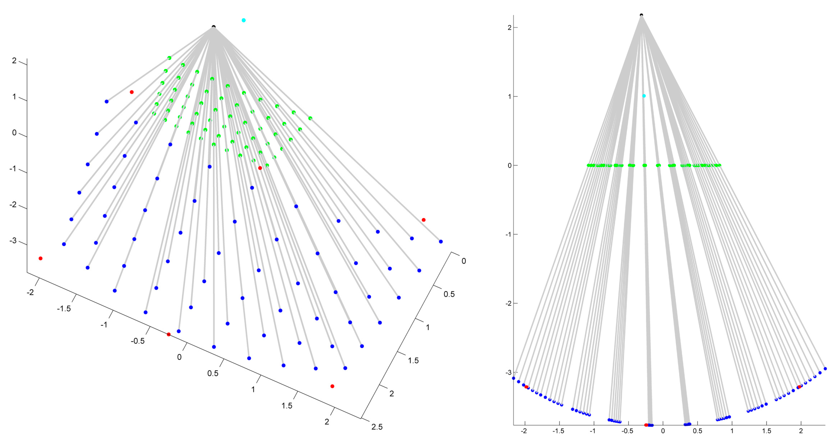
2.2.5. 2D/3D Correspondences of Chessboard
The 2D-3D correspondences required to calibrate the projectors are calculated from the set of points derived from a projected chessboard. Therefore, for the purpose of calibrating the projectors, an image of the projected chessboard on the cylinder is needed for each projector, meaning a total of three images, from which 3D coordinates will be computed by applying ray tracing: departing from the known interior and exterior camera calibration, rays are traced from the camera optical center (black dot in
Figure 5) and through each of the chessboard points at the camera image plane (green dots in
Figure 5). The intersection of each spatial ray with the vertical cylinder, which is analytically defined, results in the 3D coordinates of that point (blue dots in
Figure 5).
On the other hand, the projected image for each projector is also needed to compute 2D image coordinates of each chessboard point. The computation of the 2D coordinates with sub-pixel resolution is straightforward with pattern-based image processing techniques available in OpenCV.
2.2.6. Projector Calibration
The calibration of the projectors relies on the Direct Linear Transformation (DLT) equations. The basic model equations of the DLT are depicted in Equations (11) and (12), where
x,
y are the observable image coordinates of a point,
X,
Y,
Z are the spatial coordinates of that object point and
ai,
bi,
ci are the 11 DLT parameters of a particular image. As one observed point provides 2 equations, a minimum of 6 points are needed to solve the 11 unknowns. It is known that the DLT parameters can be directly related to the six elements of the exterior orientation parameters of an image (
X0,
Y0,
Z0, and orientation angles: camera direction
α, nadir distance
ν and swing
κ) and to five elements of the interior orientation (principal point coordinates
x0,
y0, focal length
c, relative
y-scale
λ and shear
d) [
33,
34]. Therefore, solving these equations for a minimum of 6 observed points (points with 2D-3D correspondences) leads to the computation of the interior and exterior sensor orientation. If more points are available, the system can be solved with a LSF. Finally, it is worth mentioning that the DLT fails if all CPs lie in one plane. This situation cannot occur here, as CPs lie on a curved surface, the vertical cylinder.
3. Results
3.1. Validation
The system was installed in one of the main shopping malls in València and calibrated by non-experts in-situ. The camera used in the procedure was a Canon G12 acquiring images of 2816 × 1880 resolution, which was previously calibrated at the laboratory. A total of 14 CPs were previously placed on the cylindrical surface, as indicated in
Figure 3. The measured distances are depicted in
Table 2, where the condition that all points lie on a circle has been considered by introducing the so-called fictitious observations, that in this case are distances from the center of the circle O to all CPs with the known value of the radius (as given by the manufacturer). After a LSF procedure, the compensated distances were derived (
Table 3), from which the computation of the compensated 3D coordinates of CPs is straightforward. The computed mean value of the compensated radius was 1.569 m, which is the value used in the computation of the projector calibration.
The computed interior orientation parameters of the camera and the distortion coefficients are depicted in
Table 4, which have been derived as explained in
Section 2.2.3. The exterior orientation parameters of the camera at the three positions are depicted in
Table 5, which have been derived as explained in
Section 2.2.4.
The computed interior orientation parameters of the three projectors are depicted in
Table 6, whereas the exterior orientation parameters are depicted in
Table 7. These values have been derived from the DLT parameters, as explained in
Section 2.2.6.
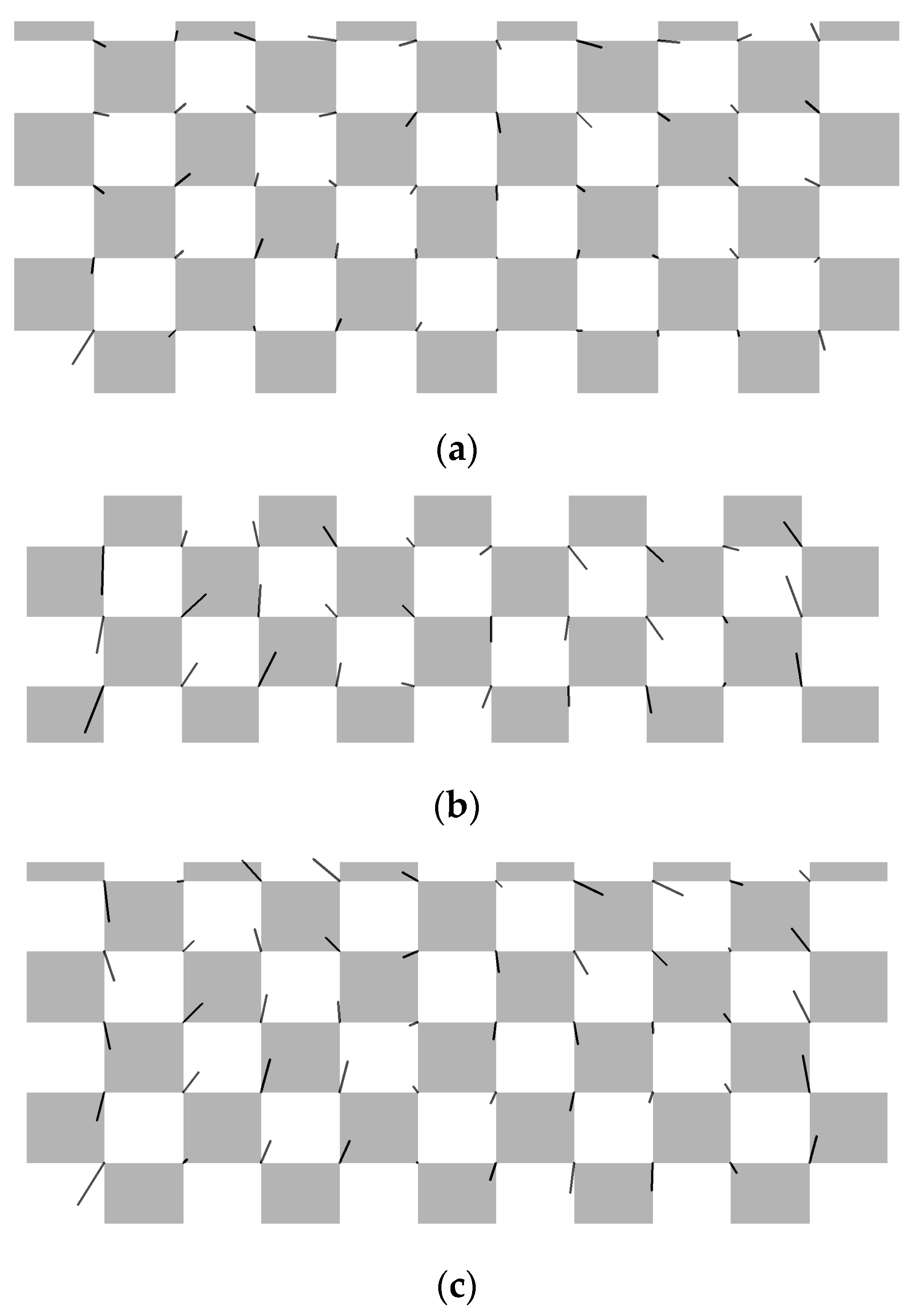
The computed average value of image discrepancies for the three projectors were 0.533 pixels, 1.056 pixels and 0.896 pixels, respectively. Individual discrepancies are depicted in
Figure 6, where a scale factor of ×50 has been applied in order to visualize the direction of the errors. As it can be noticed, there is not a predominant direction, meaning that systematic errors are not present. It can also be observed that errors at the image borders are greater than at the center of the images, but still represent low values that can be neglected.
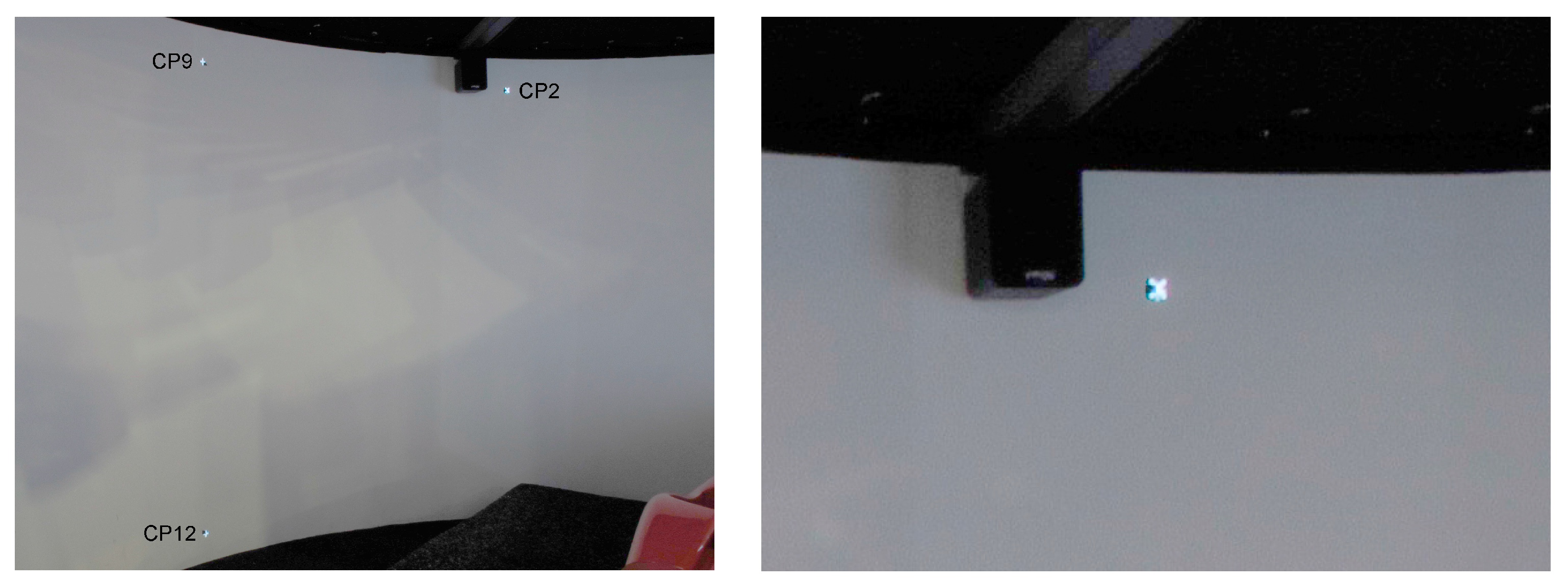
Once the projector orientation parameters have been obtained, it is possible to project onto the cylindrical surface (whose geometry is known) any point in a known 3D position. In order to further check the accuracies in object space, the computed CPs were projected on top of the physical CPs. Small discrepancies (less than 0.5 mm) were observed in object space for all cases. In
Figure 7, an image with different CPs and another detail image of CP2 are depicted, where “+” was used for Proj1 and Proj3 and “×” was used for Proj2.
3.2. Image Warping
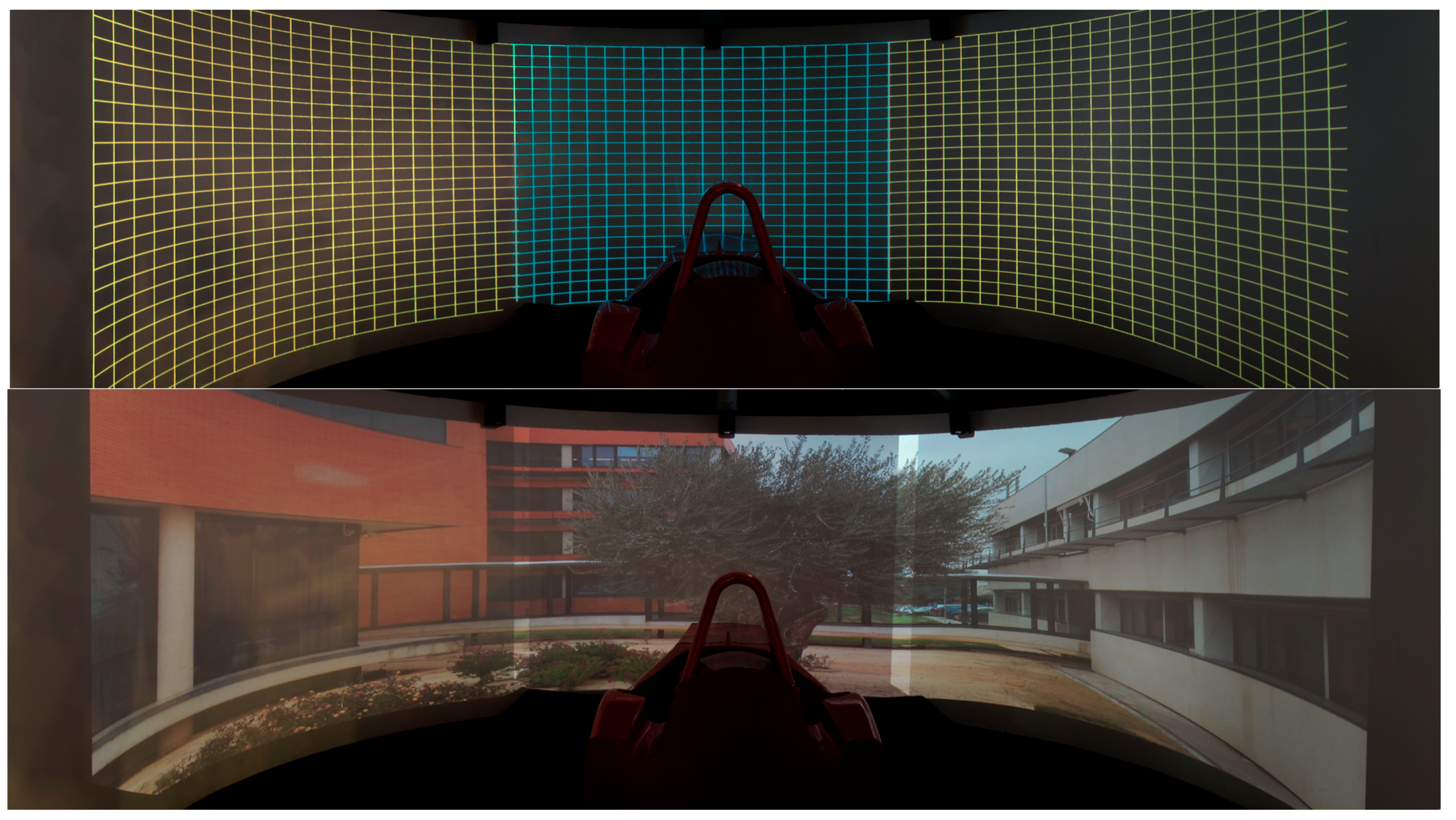
Some images were warped to the cylindrical surface with a wallpaper-like mapping, which are depicted in
Figure 8. This mapping is so called because it produces the same effect as if the image was printed on a paper and attached to the cylindrical surface following its curvature. In our implementation, the user can choose the height of the projection on the cylindrical surface and the horizontal FoV. In
Figure 8 (top) a grid is shown, where the image of the central projector is in cyan and those of the lateral projectors are in yellow. In
Figure 8 (bottom), an urban space is shown, where the overlapping between each pair of projectors is shown as it is, without applying any kind of blending in order to depict the common areas.
Although it is not part of the aim of this paper, it has to be mentioned that the overlapping areas of the projected images have to be blended. Due to the nature of most of the virtual reality simulators, the optic flow generated by the images on the screen is expected to be significantly variable (it can vary from very fast to very small). This means that the blending zone needs to be very accurate so that the mid-peripheral vision seems right to the user.
The blending process implies both a refined geometrical matching (in the overlapping areas) and a smooth photometric blending. The matching of the warping meshes obtained from the calibration is quite accurate in the overlapping areas, yet there could be room for an ultra-fine tuning. Regarding the photometric blending, a shader-based application was used to perform a linear luminance interpolation and to map the corrected wallpaper from the driving simulation output. This software reads the data obtained from the calibration process and allows also to perform small geometrical corrections to the warping mesh.
3.3. Testing the Simulator with Users
The overall system was installed in one of the main shopping malls in Valencia and tested by twenty local non-professional drivers. Each driver was prompted to use the simulator for 5 min, to avoid long runs that sometimes lead to simulator sickness. For the virtual content, we used both rFactor 2 and F1 2012, using a simulated Formula 1 car and the Reid-Nahon classical washout algorithm for the motion cueing generation.
The projection system and the screen are welded structures. The projectors and the motion platform are tightly attached to the projection structure by a series of large bolts and nuts, so the motion of the projectors with respect to the screen and the motion base is negligible. In the performed tests, none of the drivers complained about the visual perception and the matching of the images displayed by the projectors. Minor complaints were reported from some users about the lack of brightness of the image and about the vibrations of the motion cueing generation. Neither of these issues are related with the calibration process.
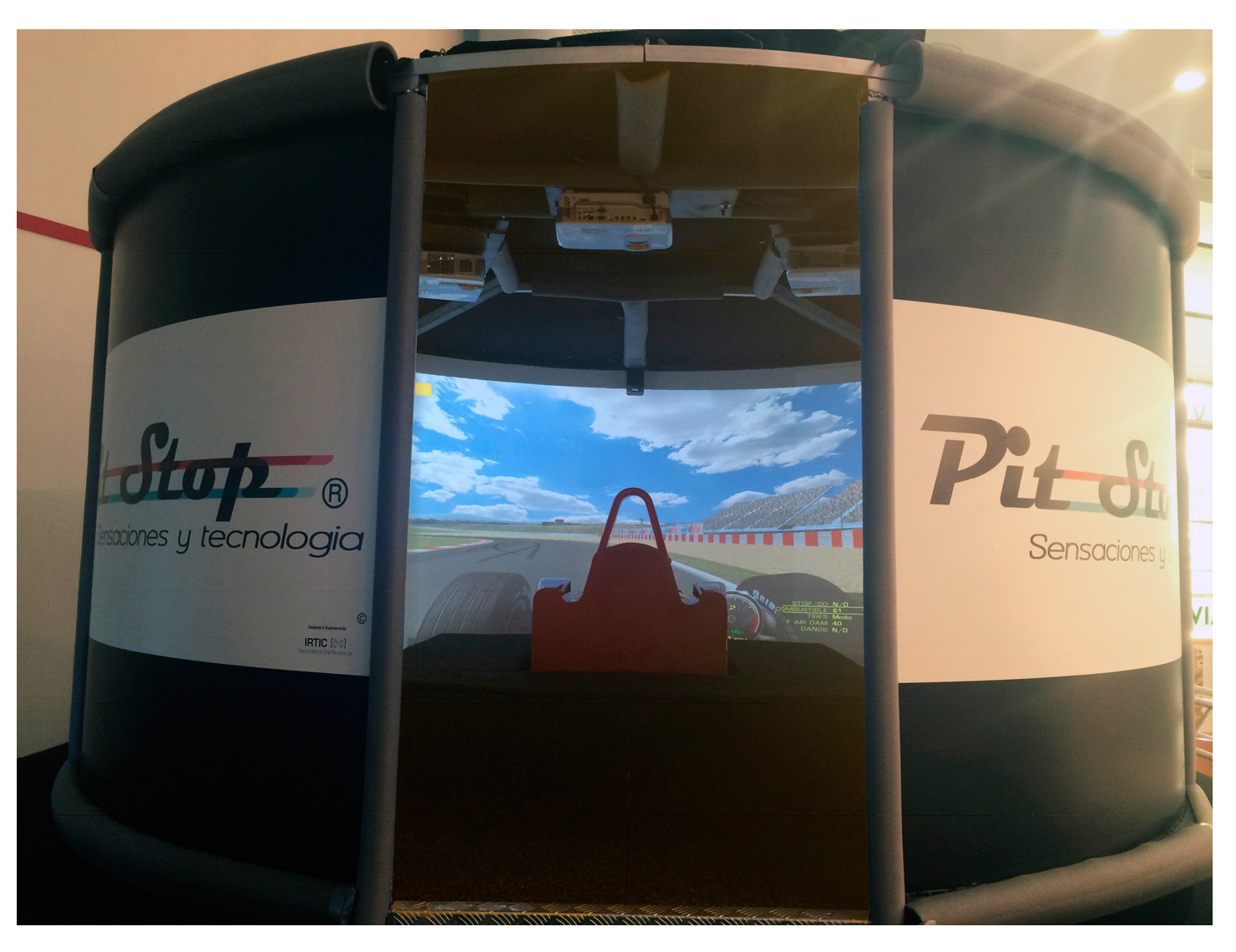
Figure 9 shows the final aspect of the system.
4. Discussion
The proposed method is a waterfall algorithm, meaning that errors of a step would not be corrected in the later process. For this reason, it is important to achieve accurate values in all the intermediate steps. For instance, if 3D coordinates of control points are not accurately achieved, the accuracy of the result might drastically worsen. In case that 3D coordinates of control points can be achieved with a total station, the errors introduced in this step can be neglected. However, if the 3D coordinates are geometrically computed after measuring distances with a measuring tape, as the sample shown here, we consider it mandatory to observe redundant distances in order to perform the LSF. In order to show the discrepancies in the computed projector orientation if LSF is not applied, we have simulated our method making use of the 3D approximate coordinates of CPs, instead of the compensated ones. The obtained discrepancies are depicted in
Table 8 and
Table 9. As it can be seen, results differ in a significant way. For instance, in case of Proj. 1 and Proj. 2, there is a discrepancy of 15 cm in the coordinate
X0, while differences in angular values arrive to 10 degrees in some cases.
It is also relevant to mention that the reason why we used three camera positions is because of the spatial restrictions imposed by the F1 simulator. However, this method could be used to calibrate multiple projectors with a single camera position, provided that the FOV of the camera captures the whole screen at once. In such a case, only one input image and a minimum of 4 CPs would be needed to calibrate the camera. Once the camera is calibrated, the rest of the method can be applied as here explained.
Finally, we would also like to mention that, although the method here presented works for any kind of analytically defined screens, it could be easily adapted to any kind of screens, even irregular surfaces. In this case, instead of mathematically defining the surfaces, the surfaces can be given as a cloud of points. Thus, in order to achieve the 3D chessboard object coordinated of CPs, ray tracing can be applied as here proposed, but by intersecting the cloud of points. This is easily solved by just finding the closest point to the 3D ray. We propose this as future work.
5. Conclusions
Multi-projector setups are used in many different applications, such as virtual reality visualizations, projected augmented reality or 3D reconstruction, among others. This paper presents a fast and easy-to-use method to calibrate a multi-projector system for analytically defined screens.
We have developed and presented the equations for a cylindrical screen, and tested the process in a real case where multi-project calibration is needed: a real-time Formula 1 simulator.
The contribution of our work lies in the simplicity of the process from the point of view of the person in charge of performing the calibration process. We also perform the calibration on the actual screen being calibrated, without the need to move it or use auxiliary surfaces. The measuring process is easy and requires neither dedicated infrastructures nor complex tools. In contrast to other calibration methods, our calibration process can be performed by any person capable of using a measuring tape. The most complicated step may be the camera calibration, although this is done only once and can be performed offline at the laboratory.
Moreover, the time needed to obtain the calibration parameters is also kept small, although electromechanical calibration methods are usually faster (but much more expensive). Both the measuring and the computation process require little time to complete. In fact, the mathematical methods needed to complete the process are computable in a few seconds by a modern computer, so the more time-consuming task of our calibration method could be the manual measuring of the distances between the CPs.
While being simple, the method is accurate enough for most of the applications where calibration is needed. Image discrepancies are around or less than one pixel, and systematic errors are not present. Our aim is entertainment and virtual reality, areas where the amount of accuracy we obtained are sufficient. Other scientific areas, such as metrology, may require higher accuracy. However, accuracy comes at a cost.
In addition, although we presented here the evaluation for a cylindrical screen, the method could be applied to other analytical shapes, such as spheres or conical surfaces. Our method cannot be applied to planar screens (at least in the current form presented here), as DLT equations fail on co-planar points. However, we are not interested in this type of screens, because the majority of screens used in immersive virtual reality applications are either cylindrical or spherical. This is even truer in real-time simulators, like the one we used for our tests. The method can also be applied to non-analytical surfaces by making use of cloud point ray tracing, but these kinds of surfaces are unusual in virtual reality or entertainment applications.


