Glidar: An OpenGL-based, Real-Time, and Open Source 3D Sensor Simulator for Testing Computer Vision Algorithms

Abstract

3D sensors such as lidars, stereo cameras, time-of-flight cameras, and the Microsoft Kinect are increasingly found in a wide range of applications, including gaming, personal robotics, and space exploration. In some cases, pattern recognition algorithms for processing depth images can be tested using actual sensors observing real-world objects. In many situations, however, it is common to test new algorithms using computer-generated synthetic images, as such simulations tend to be faster, more flexible, and less expensive than hardware tests. Computer generation of images is especially useful for Monte Carlo-type analyses or for situations where obtaining real sensor data for preliminary testing is difficult (e.g., space applications). We present Glidar, an OpenGL and GL Shading Language-based sensor simulator, capable of imaging nearly any static three-dimensional model. Glidar allows basic object manipulations, or may be connected to a physics simulator for more advanced behaviors. It permits publishing to a tcp socket at high frame-rates or can save to pcd (point cloud data) files. The software is written in C++, and is released under the open source bsd license.

1. Introduction

Sensors that produce three-dimensional (3D) point clouds of an observed scene are widely available and routinely used in a variety of applications, such as self-driving cars [1], precision agricultural [2], personal robotics [3], gaming [4], and space exploration [5,6]. This widespread use is a direct result of a series of advancements in 3D imaging technologies over the last few decades that has both increased performance and reduced cost.

There are a variety of different types of 3D sensors, each using a different operating principle to generate the 3D point clouds or depth maps. Early systems were primarily based stereovision (comparing images from two cameras separated by a known baseline) [7], but have recently given way to active sensors. Of particular note are time-of-flight cameras [8,9], lidars [6], and structured light sensors (as exemplified by the Microsoft Kinect) [4,9].

Falling prices and the increased availability of these 3D imaging technologies have motivated development of such resources as the Point Cloud Library (pcl) [10] as well as new 3D-specific algorithms in the OpenCV library [11,12].

With the proliferation of 3D sensors and the associated pattern recognition algorithms has come a need for easy ways of testing new approaches and techniques. The most straightforward way of obtaining the required test data would be to collect imagery of a real-world object using the specific sensor of choice. This approach comes with a variety of challenges. First, although many 3D sensors are now quite affordable, some of these sensors (e.g., lidars) are still too expensive for many research groups to easily purchase. Second, analyzing the performance of algorithms with data from an actual sensor often requires precise knowledge of the sensor–object pose as well as a detailed 3D model of the observed object. Obtaining such information can be tedious, time consuming, and can significantly impede rapid testing early in the design process. Third, images produced by real sensors have noise and a variety of artifacts associated with their unique operating principles. While the handling of such idiosyncrasies is important for mature algorithms that will be used in practical settings, we frequently want to control the introduction of such effects during algorithm development and testing. Fourth, hardware-based tests are ill-suited for supporting large statistical analyses of algorithm performance, such as in Monte Carlo analyses [13]. Fifth, and finally, some scenarios are extremely difficult to test in the laboratory environment—especially those involving space applications where the scale, lighting, dynamics, and scene surroundings are challenging (and expensive) to accurately emulate on Earth [14,15,16].

For these reasons it is often preferable to test new algorithms via simulation, only moving to hardware tests when algorithms are more mature. Compared to the hardware-based testing described above, depth images created through computer simulation are cheaper, more flexible, and much faster. Thus, a simulation-based approach is ideal for algorithm development, performance analysis, incremental introduction of error sources, and large Monte Carlo-type analyses in which an algorithm may need to be run tens of thousands of times with randomly varying inputs.

Yet, to our knowledge, no software has been made freely available to the general public for the emulation of a generic 3D sensor—that is, for the easy and rapid generation of simulated depth images from 3D models. While there are good open-source tools for processing and editing point clouds (e.g., MeshLab [17]), these are typically more suited for handling existing point clouds rather than generating the point clouds (or depth maps) that would be created by a 3D sensor. It is also not desirable to generate a measured point cloud directly from the observed model vertices, since we desire the point cloud to describe where the sensor would actually sample the surface rather than simply where the model happens to have mesh vertices. As a result, various research groups are left to independently redevelop such a capability, leading to much duplication of effort and lack of a common tool. We address this problem by presenting Glidar (a portmanteau of OpenGL and lidar), which is capable of loading 3D models in a variety of formats, re-orienting them, and saving depth images of the visible surfaces (Figure 1). Glidar is written in C++ and makes use of the graphics rendering pipeline included in most modern personal computers via the GL Shading Language (glsl), which confers sufficient speed that it may be used as an input for nearly any algorithm which processes point cloud data.

Glidar does not simulate any specific piece of hardware. It can, however, be used in lieu of nearly any 3D sensor and can generate synthetic point clouds of whatever model object the user chooses to load (a few illustrative examples are shown in Figure 2). Glidar permits point clouds to be saved as files, visualized, or published to a Transmission Control Protocol (tcp) socket. Additionally, this software—if more complicated dynamics than constant rotation are desired—may optionally subscribe (via tcp) to a physics simulation.

While other groups have utilized graphics hardware to produce radar and lidar sensor simulators in the past [18,19,20], Glidar appears to be the only piece of software available for free public download. Thus, the purpose of this short note is to introduce the imaging community to Glidar and to document key aspects of its present implementation. It is our hope that our software — released under an open source license — will be of use to others, and that users might submit patches and improvements.

Figure 1. Glidar uses the green and blue channels to store depth information (top left) and outputs a point cloud sampled from the visible surfaces of the object (displayed from a variety of angles and ranges on the right). Shown at bottom left is a normal 3D rendering of the original model, the Stanford Bunny, which is available from the Stanford 3D Scanning Repository [21].

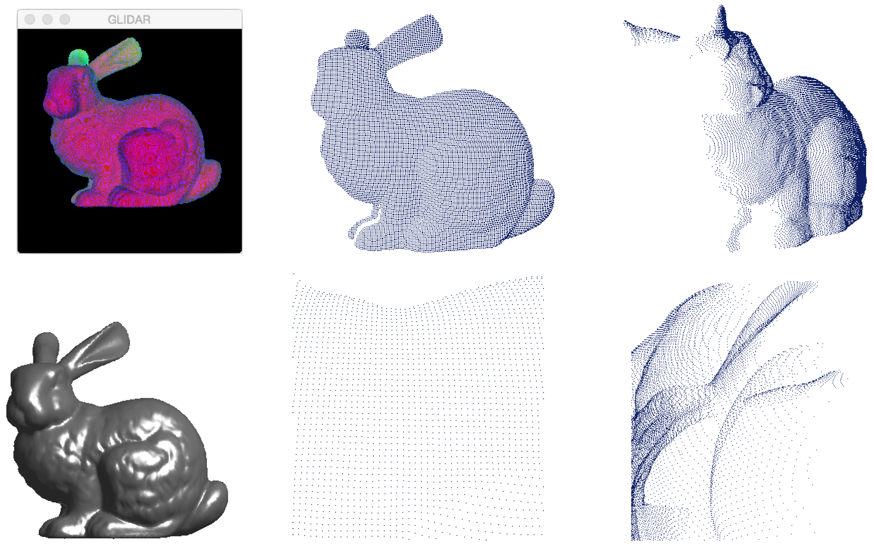
Figure 1. Glidar uses the green and blue channels to store depth information (top left) and outputs a point cloud sampled from the visible surfaces of the object (displayed from a variety of angles and ranges on the right). Shown at bottom left is a normal 3D rendering of the original model, the Stanford Bunny, which is available from the Stanford 3D Scanning Repository [21].

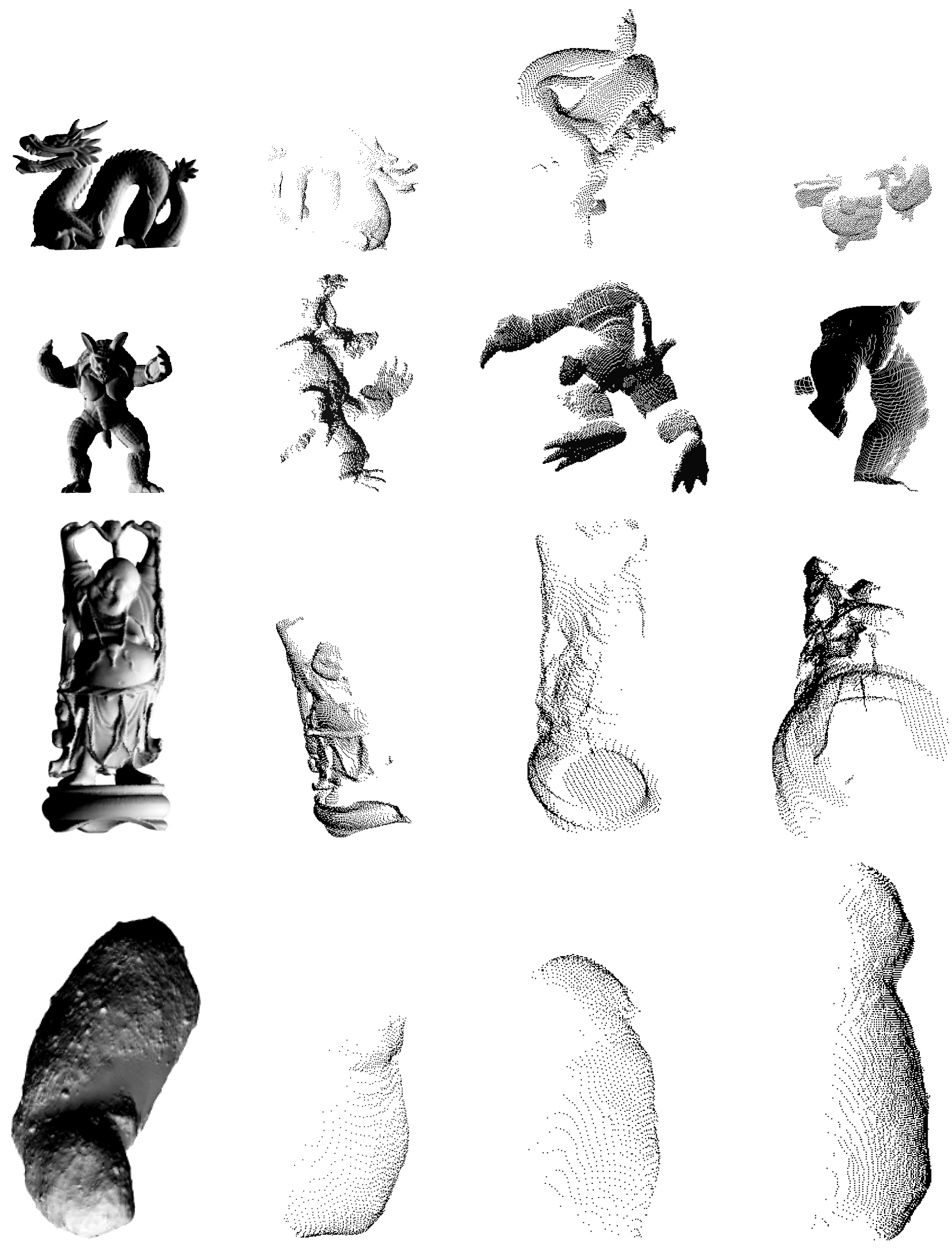
Figure 2. Glidar can quickly produce depth images of objects from different orientations, with differently shaped and sized fields of view, and at a variety of ranges. The left-most column consists of four models which we used to produce the point clouds in the other columns. The first three models (Dragon, Armadillo, and Happy Buddha) are from the Stanford 3D Scanning Repository [21]. The fourth is the asteroid 25143 Itokawa, and was obtained from then the NASA Planetary Data System [22] and glued together and exported into ply format using Blender [23].

Figure 2. Glidar can quickly produce depth images of objects from different orientations, with differently shaped and sized fields of view, and at a variety of ranges. The left-most column consists of four models which we used to produce the point clouds in the other columns. The first three models (Dragon, Armadillo, and Happy Buddha) are from the Stanford 3D Scanning Repository [21]. The fourth is the asteroid 25143 Itokawa, and was obtained from then the NASA Planetary Data System [22] and glued together and exported into ply format using Blender [23].

2. Algorithms

Glidar’s design is based on a fairly standard pattern for OpenGL applications (which will not be explored in great detail here). In general, the current design does away with color information, utilizing the red channel for intensity and the green and blue channels to store the z depth (the camera frame convention used here assumes that the +z direction is out of the camera and along the camera boresight direction).

We elected not to use the standard depth buffer to store depth information, as this portion of the pipeline was not easily customizable within the graphics architecture on which we developed Glidar (a 2011 MacBook Air). The default behavior for the OpenGL depth buffer is to provide the most precision near the camera, and less further away; but we wanted the precision to be equal for points near and far away, and using the color buffer allowed us to directly specify the precision distribution.

Two key modifications to the standard pipeline were necessary: we turned off antialiasing to avoid modifying the depth information stored in the green and blue channels, and enabled double-buffering (it could, perhaps, be disabled if we wished to crudely simulate a scanning lidar). This section focuses on the less conventional aspects of the rendering pipeline, namely the glsl shaders and “unprojection” of the depth information.

2.1. The Programmable Rendering Pipeline

The vertex and fragment shaders, first proposed by [24], are standard parts of the modern rendering pipeline—but are nevertheless worth explaining for the purposes of the discussions that follow.

Primitive objects (points, lines, and polygons) are specified in terms of vertices, but the graphics hardware must provide per-pixel output. Rendering is split into multiple passes, with the least frequent operations (e.g., primitive group) occurring first; the per-primitive group outputs are then processed by the vertex shader in parallel across each vertex. The vertex shader outputs are assembled into primitives for rasterization. Finally, the vertex shader’s outputs are interpolated on a per-pixel basis in the fragment shader, where they may be used to compute color, texture, and depth information for each pixel (fragment).

For the purposes of this discussion and for notational convenience, we present the per-vertex operations as if they were global, and per-fragment operations with a subscript i—since the per-fragment computations are performed on interpolated values from the vertex shader. However, it is worth noting that graphics processing units compute each vertex in parallel, and then each fragment in parallel.

In the standard shading models, some basic compromises are made to model the amount of light reflected toward the viewer. For example, [25] shading uses $\overrightarrow{r}·\overrightarrow{v}$, which must be recalculated for each fragment. In Blinn–Phong shading [26], the expression is $\overrightarrow{n}·\overrightarrow{h}$, where $\overrightarrow{n}$ is the surface normal, and

$$\overrightarrow{h}=\frac{\overrightarrow{l}+\overrightarrow{v}}{\parallel \overrightarrow{l}+\overrightarrow{v}\parallel }$$

(1)

is termed the halfway vector, or simply the half-vector; here, the vector to the viewer is $\overrightarrow{v}$, and the light source vector is $\overrightarrow{l}$. (The notation $\parallel \overrightarrow{x}\parallel$ indicates the 2-norm length of vector $\overrightarrow{x}$).

However, when the light source is approximately co-located with the viewer, as in many 3D sensors, we can use the equivalent computation

$$\overrightarrow{h}=\frac{\overrightarrow{l}}{\parallel \overrightarrow{l}\parallel }$$

(2)

simply the normalized light vector, for each vertex—a value that is next interpolated into ${\overrightarrow{h}}_i$ for each fragment i.

2.2. Fragment Shader

A typical fragment shader calculates the color and alpha (transparency) of each pixel, or fragment, in an image based on values from the vertex shader. Such a fragment shader would output four values for each fragment: normalized intensities for each of red, green, and blue, and an alpha.

In contrast, the Glidar fragment shader outputs only the red value, and uses the green and blue channels to provide the z depth (the length of $\overrightarrow{l}$ projected onto boresight direction) interpolated at each fragment; alpha is currently unused (Figure 1).

Attenuation a is calculated for each fragment i using the standard OpenGL lighting model,

$$a_i={\left(a_{\mathrm{C}}+a_{\text{L}}{d}_i+a_{\mathrm{Q}}{d}_i^2\right)}^{-1}$$

(3)

where $d_i=\parallel {\overrightarrow{l}}_i\parallel$ is the fragment–sensor (or fragment–light) distance, and $a_{\text{C}}$, $a_{\text{L}}$, and $a_{\text{Q}}$ are respectively the constant, linear, and quadratic attenuation values for the light source.

Per-fragment red intensity

$$r_i=a_i{c}_i$$

(4)

is then the product of attenuation and color,

$$c_i=\left(c_{\text{A}}+c_{\text{D}}max({\overrightarrow{n}}_i·{\overrightarrow{h}}_i,0)+c_{\text{S}}max{({\overrightarrow{n}}_i·{\overrightarrow{h}}_i,0)}^s\right)$$

(5)

with ${\overrightarrow{n}}_i$ as the surface normal at the fragment being sampled (interpolated from the vertex normals in the vertex shader), and $c_{\text{D}}$, $c_{\text{A}}$, and $c_{\text{S}}$ representing the diffuse, ambient, and specular color information (which depend on both the light source and the object’s textures and materials), respectively. The material’s shininess (a term specific to graphics pipeline specifications) is described by s and is used to adjust the relative influence of the specular component in Equation (5). OpenGL allows values of s in the range $[0,128]$.

We used the green channel to store the most significant bits and the blue to store the remainder. In other words, the green and blue intensities for each fragment i—with each able to hold one byte, and in the range $[0,1]$—are

$$\begin{array}{ccc}\hfill g_i& =& \frac{⌊\frac{D_i}{256}⌋}{256}\hfill \end{array}$$

(6)

$$\begin{array}{ccc}\hfill b_i& =& \frac{D_{i}mod256}{256}\hfill \end{array}$$

(7)

where $D_i$ is the distance ratio for the fragment; we define

$$D_i=65536\frac{{\omega }_i{d}_i-n}{f-n}$$

(8)

where ${\omega }_i$ is the projection of the light vector direction for the i-th fragment onto the camera boresight direction $\overrightarrow{s}$ and is computed according to

$${\omega }_i=\frac{\overrightarrow{s}}{\parallel \overrightarrow{s}\parallel }·\frac{{\overrightarrow{l}}_i}{\parallel {\overrightarrow{l}}_i\parallel }$$

(9)

Thus, the term ${\omega }_i{d}_i$ finds the z depth (or the z-axis coordinate) of the i-th fragment as expressed in the camera frame. Again recall that the camera boresight is defined to be along the camera frame’s positive z-axis direction. The values n and f in Equation (8) represent the near and far plane z depths, respectively, in the camera frame. We see, therefore, that our equation for $D_i$ automatically scales the depth value stored for each fragment such that we obtain the best possible resolution given our 16-bit expression of depth (8 bits from the green channel and 8 bits from the blue channel).

2.3. Strategies for Improving Depth Accuracy

In a standard OpenGL depth buffer, greater precision is afforded to points in a scene which are closer to the camera. This default behavior, while useful for 2d rendering, produces point clouds with noticeable depth banding—that is, the depths in a 3D image appear to be quantized when the scene is rendered (see Figure 3). Quantization is reduced, but not eliminated, in two ways:

• use of both the green and blue channels (as described above) to store depth information, and
• adjusting the near and far plane locations to hug the object-of-interest as tightly as possible.

As such, the current release of Glidar is capable of rendering only one object at a time. Adaptations for rendering entire scenes would require major revisions to our approach for (2).

Figure 3. Depth quantization, in the form of banding, occurs without significant customizations to the storage of depth information. This point cloud is sampled from a fake rock model, using only the blue channel for depth, and without the other adjustments we made for improving the depth accuracy.

Figure 3. Depth quantization, in the form of banding, occurs without significant customizations to the storage of depth information. This point cloud is sampled from a fake rock model, using only the blue channel for depth, and without the other adjustments we made for improving the depth accuracy.

3. Discussion

Glidar has been tested on several Ubuntu Linux machines as well as on Mac OS X (both Mavericks and Yosemite). It requires a graphics card with support for glsl 1.2 or higher.

The software also makes use of a number of open source libraries, and requires cmake, Opengl Mathematics (glm) and Eigen, glew, glfw, ømq, assimp, ImageMagick/Magick++, and pcl. Some of these requirements, such as Eigen (which is used for matrix and vector operations), are deprecated by our use of glm, and will be removed in a future release. Additionally, pcl is mainly used for parsing command line arguments (and was used for convenience as part of our own pipeline), but may be dispensed with easily.

Perhaps the most important of the software requirements is the Open Asset Import Library (assimp) [27], which is responsible for loading 3D models in an array of formats—thus, Glidar works with most models assimp is able to load. Additionally, our software makes use of Magick++ for loading textures (Figure 4), particularly bump textures, which greatly improve the fidelity of the rendered 3D images by providing normal information for the object models.

In future versions, we hope to develop a texture-based noise model for simulating sensor noise; for a proof of concept generated using Glidar, see Figure 5. Two simple noise models are included in the current version, but both are currently disabled in the fragment shader, and neither has been tested extensively.

Figure 4. Glidar can apply model texture information to affect the intensity and normals of a model when producing depth images. In this illustration, the solar panel textures from the International Space Station’s Functional Cargo Block module are visible as differing intensities in the point cloud. The texture map used in this example is meant to be illustrative of Glidar’s capability to consider texture, rather than to represent the actual appearance of such an object; accurate representation of structures in the near-infrared would likely require generation of custom textures. This particular model is a component of Nasa’s high-resolution iss scene in Lightwave format, obtained from [28].

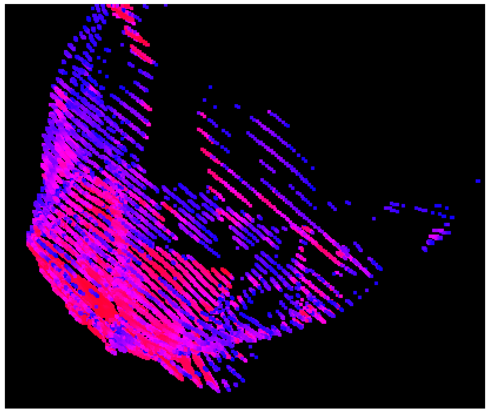
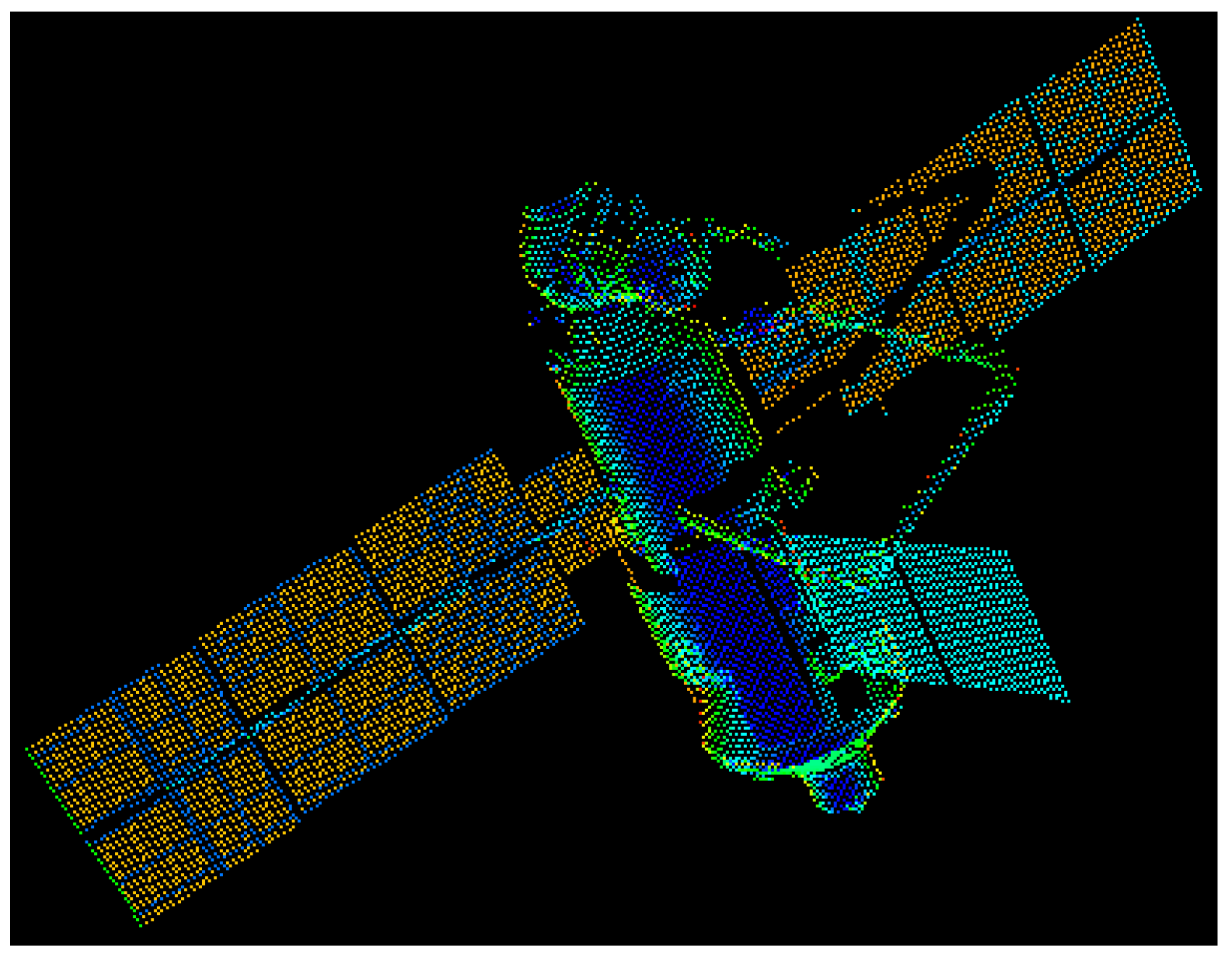
Figure 4. Glidar can apply model texture information to affect the intensity and normals of a model when producing depth images. In this illustration, the solar panel textures from the International Space Station’s Functional Cargo Block module are visible as differing intensities in the point cloud. The texture map used in this example is meant to be illustrative of Glidar’s capability to consider texture, rather than to represent the actual appearance of such an object; accurate representation of structures in the near-infrared would likely require generation of custom textures. This particular model is a component of Nasa’s high-resolution iss scene in Lightwave format, obtained from [28].

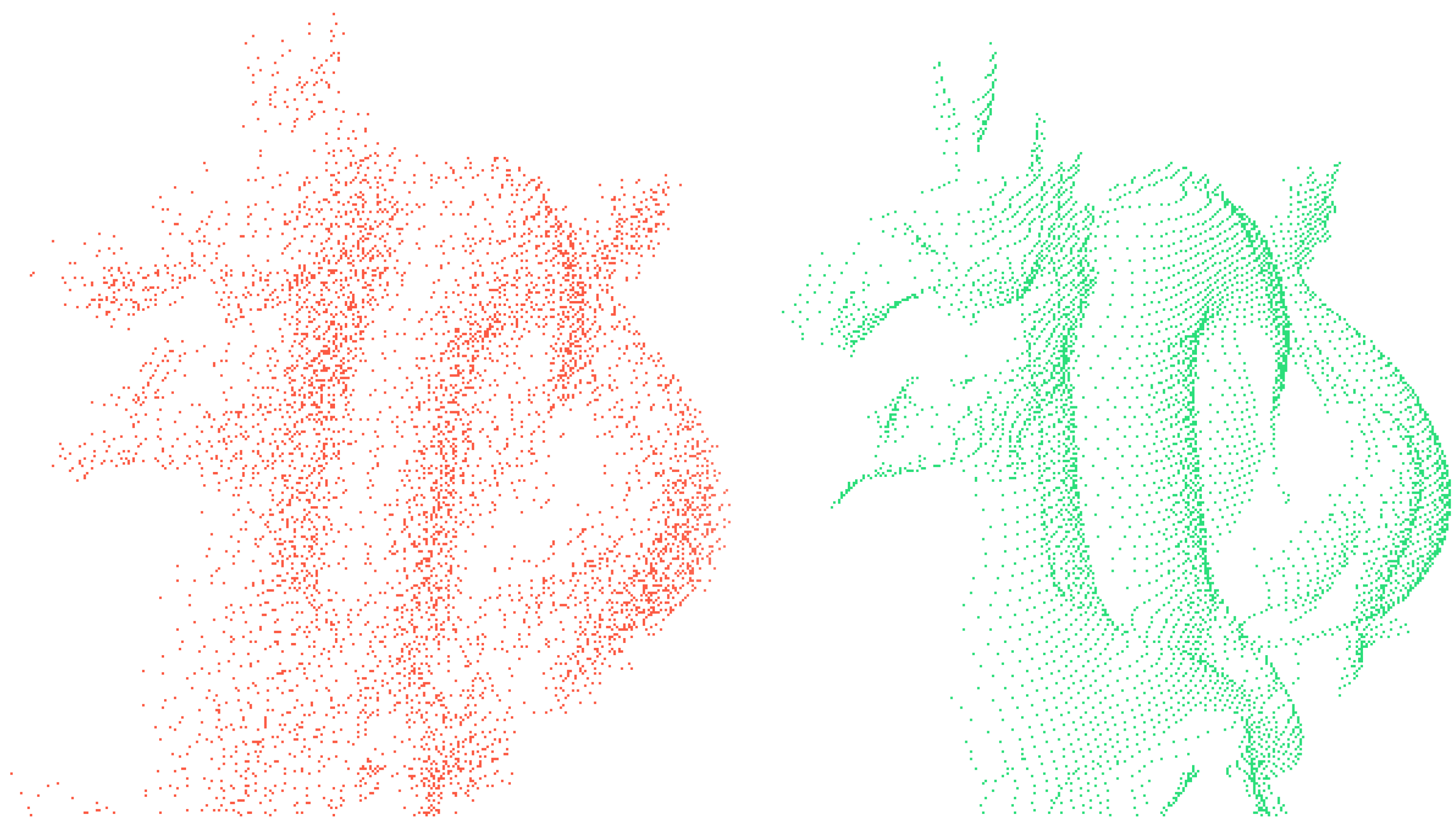
Figure 5. An additive noise model may be included in the fragment shader to apply device-specific range errors. Shown above are point clouds sampled from the Stanford dragon, with additive noise (left) and without any noise (right). We hope to include texture-based noise in the future.

Figure 5. An additive noise model may be included in the fragment shader to apply device-specific range errors. Shown above are point clouds sampled from the Stanford dragon, with additive noise (left) and without any noise (right). We hope to include texture-based noise in the future.

Another area where Glidar is not particularly useful is in dealing with deformable models, such as plants, animals, and faces, which are outside the scope of our research team’s present needs. However, we encourage others to submit improvements.

Although Glidar is not designed to simulate any specific sensor, we find it to be a useful asset for testing and characterizing algorithms that work on point clouds (e.g., iterative closest point, [29]). We hope that future work will further increase the utility of this new software, which may be downloaded from Github at http://github.com/wvu-asel/glidar.