Parameter Optimization for Local Polynomial Approximation based Intersection Confidence Interval Filter Using Genetic Algorithm: An Application for Brain MRI Image De-Noising

Abstract

Magnetic resonance imaging (MRI) is extensively exploited for more accurate pathological changes as well as diagnosis. Conversely, MRI suffers from various shortcomings such as ambient noise from the environment, acquisition noise from the equipment, the presence of background tissue, breathing motion, body fat, etc. Consequently, noise reduction is critical as diverse types of the generated noise limit the efficiency of the medical image diagnosis. Local polynomial approximation based intersection confidence interval (LPA-ICI) filter is one of the effective de-noising filters. This filter requires an adjustment of the ICI parameters for efficient window size selection. From the wide range of ICI parametric values, finding out the best set of tunes values is itself an optimization problem. The present study proposed a novel technique for parameter optimization of LPA-ICI filter using genetic algorithm (GA) for brain MR images de-noising. The experimental results proved that the proposed method outperforms the LPA-ICI method for de-noising in terms of various performance metrics for different noise variance levels. Obtained results reports that the ICI parameter values depend on the noise variance and the concerned under test image.

1. Introduction

Brain MR Image analysis is a common clinical activity which is used to diagnose many neurological diseases such as Alzheimer’s disease, multiple sclerosis, brain tumor, etc. A computer-aided system helps automating this clinical activity in order to obtain faster and reliable analysis. Recently, an imperative research is focused on the medical image processing in various fields such as [1,2,3,4].

Generally, Magnetic resonance imaging (MRI) is one of the most noninvasive medical imaging powerful modalities endow with highly detailed images of organs and tissues in the human body. It produces detailed images of organs, bone, soft tissues, brain, and all other internal body structures. MRI facilitates the discovery of abnormalities which might be obscured by bone with other imaging methods. However, these MRI images are undergoing numerous noise sources, such as a transmission medium, recording medium (digital sensor, film) and measurement/ quantization errors [5], ambient noise from the environment, acquisition noise from the equipment, breathing motion, body fat, RF coil, RF pulses, the presence of background tissue, field strength, receiver bandwidth, etc.

Consequently, the MRI acquired directly from the instruments is commonly inadequate for medical analysis, especially in brain and cardiac [6] because of the existence of high levels of Rician noise [7,8] that degrade the image quality. As a corollary, to achieve consistent analysis, removing MRI image noises is compulsory before conducting any supplementary image processing such as registration, segmentation, classification, and visualization.

Noise modeling is significantly influenced by the capturing instruments. Diverse algorithms are employed based on the noise model. For supplementary analysis, pre-processing and appropriate diagnosis necessitates the development of de-noising methods to refine the image quality and increase the Signal-to-Noise Ratio (SNR).

Recently, removing the noise from images to restore the original image is considered as a serious challenge that has a sturdy research [9,10]. Enormous techniques using variety algorithms used for MRI medical images de-noising, some of them are as follows.

Wavelet methodology has enormous uses in diverse areas as presented in [11,12], as well as it proved its efficiency in de-noising of MRI images as follows. Healy and Weaver [13], dealt with soft-thresholding based on wavelet techniques for de-noising MR images. While, Nowak [14], studied that the square magnitude MRI image, contains a Rician noise model in the threshold-based wavelet de-noising approach to correct the bias produced by the noise.

Through the year 2003 [15], the authors suggested MRI image de-noising technique using adaptive wavelet thresholding. To amplify the significant features, this method multiplied the adjacent wavelet sub bands, and then applied threshold to the multi-scale products to differentiate edge structures in an improved approach from noise. Results of MRI images proved that this method achieved high mean-to-standard-deviation ratio (MSR) and contrast to noise ratio (CNR). During the same year, Jiang et al. [16] was presented a background-noise modeling using a Rician distribution. Then, the authors employed the parameter estimation via a Maximum-Likelihood method. Both simulated and real MRI image results proved that the proposed method outperformed other de-noising approaches. Based on spectral subtraction for noise removal in functional magnetic resonance imaging (fMRI) data in [17], the author presented an adaptive signal-preserving technique. The introduced technique had estimated a parametric model for the power spectrum of the random noise from the obtained data derived from the characteristics of the Rician statistical model. The results demonstrated the potential of the suggested method in noise suppression. Meanwhile, a de-noising algorithm for medical images had been proposed in [18], based on a combination of both the wavelet and the total variation minimization methods. In real noisy medical images, results showed that the proposed algorithm offers effective noise removal. As a supplement, this algorithm permitted the implementation of an effective automatic stopping time criterion extensively.

Manjon et al. [19] employed spatial averaging for similar pixels. The authors utilized information from all available image components to perform the de-noising process. Later, Rajeesh et al. [20] used wave atom shrinkage for MRI images de-noising. The authors established that curvelet shrinkages were better than the wavelet method, as the proposed approach had achieved better SNR. Furthermore, the effectiveness of the proposed method was accentuated with large dataset of real-time normal and pathological MR images.

A review of the noise reduction algorithms for brain MRI images was presented in [21]. The anisotropic diffusion filtering reduces the noise as well as erased the small feature due to its edge enhancement. Another filter type using the spectral subtraction method was performed after acquiring signals from each RF coil separately with less acquisition time [22]. The results showed enhanced signal to noise ratio (SNR) up to 40% in the MRI reconstructed signal.

Meanwhile, the authors in [23] implemented a de-noising algorithm on MR brain images. The proposed de-noising algorithm was concerned with the poor quality images manipulation as well as to improve the deteriorated SNR. The noise was removed from the MRI images using the median filter, the weighted median and the adaptive filter. Lastly, the evaluation performance of these filters showed that using the weighted median filter was outperforming the other filters with peak signal to noise ratio PSNR = 0.924.

Iftikhar et al. [24] proposed a novel improved adaptive nonlocal means (IANLM) algorithm. The authors employed a window adaptation test based on robust threshold criterion that used to select the appropriate pixels for the restoration process. The experimental results were performed at various noise levels of simulated real brain MR images. It is established that the proposed algorithm was better for de-noising jointly with its efficient computation due to proposed modifications. In the year 2014 [25], the authors suggested an enhanced non-local means (ENLM) algorithm as an extension for the previously mentioned IANLM algorithm for brain MRI images with Rician noise. Results proved the superiority of the ENLM compared to other de-noising methods. By adapting the IANLM method [26], an extended nonlocal means (XNLM) algorithm was used to Rician noise in MR images. Furthermore, a wavelet coefficient mixing process was used in the XNLM to mix the wavelet sub-bands of two IANLM-filtered images. Lastly, the XNLM consists of new parameter-free pixel pre-selection method which improved the algorithm computational efficiency.

Most of these algorithms used low-pass filtering and averaging to achieve de-noising, where high frequency coefficients can be removed by filtering. At the same time, since edges also have high frequency components, thus during removing the noise, high frequency components of the edges are also removed. Therefore, using weighted median filters conserved edges while removed noise as proved. Consequently, Klepaczko in 2013 [27], proposed a novel scheme based on the local polynomial approximation (LPA) filter for de-noising to design GPU hardware. Relevance of LPA to high-resolution 3D MR images occurs inefficient. Thus, the author proposed parallelized GPU-accelerated implementation of LPA to remove the noise from the MR data effectively and efficiently. The author concluded that the emphasized designed GPU-based performance of the LPA algorithm was achieved very powerfully. Accomplished within a time frame reduced to milliseconds, generation of LPA masks, no longer entails any significant computational load to Shape-Adaptive Discrete Cosine Transform (SADCT) based noise removal method.

As a consequence, the LPA is efficient for MRI brain images de-noising as it is a non-parametric algorithm. It was implemented in various image processing applications [28,29].The key parameter of the LPA is the choice of its window size (scale), where a signal is convolved with a kernel function of a known form to estimate the values in the locality of a given data point. For adjusting the window size to be adapted to the local image contents, an intersection of confidence intervals (ICI) rule can be used. This LPA-ICI algorithm for image de-noising has various parameters to be adjusted to determine the optimal window size. One of these parameters is Gamma Γ, which has an infinite range. Besides, other parameters are known to be adjusted. Thus, the key idea of the proposed work is to employ an optimization procedure that can be used to adjust the LPA-ICI parameters for each MRI brain images.

Recently, a variety of optimization algorithms have been used in the medical imaging area such as in [30,31,32,33,34,35]. Consequently, Misra et al. proposed a method where the noise-reduction filtering is realized by Genetic Algorithm [36]. The genetic operator combines the crossover and adaptive mutation to improve the convergence rate as well as the solution quality of the GA. The suggested technique successfully diminishes the standard deviation and considerably lowers the rectified noise. Meanwhile, by the year 2014, Liu et al. conducted a medical image de-noising method using GA based on wavelet threshold [37]. To obtain the optimal threshold, the authors used a GA combined with clustering histogram of the image information. Experimental results proved the improved visual effect of medical image after de-noising and the improved peak signal to noise ratio when using the ordinary wavelet threshold demising method.

Consequently, this work will merge both the Genetic Algorithm optimization technique to support LPA-ICI de-noising filter (LPA-ICI-GA) by selecting the optimized ICI parameters for Rician noise removal. Where, genetic procedures including reproduction, crossover, and mutation are applied to increase the signal-to-noise ratio and minimize the overall computational complexity through using the mean square error (MSE) as the cost function. The main advantage of the GA compared to other optimization algorithms is its robustness. Jointly with, it requires less number of iterations for convergence [38]. Therefore, the contribution of this work is the optimization based GA that used to select the optimal parameters of the LPA-ICI filter. In addition, the supposed benefit of this research is to obtain better PSNR and system performance compared to the LPA-ICI itself.

The remaining sections are organized as follows. Section 2 introduces the Rician distributed noise model and the MR signals de-noising. Then, Section 3 presents the methodology that includes the image de-noising using LPA-ICI and the genetic algorithm for optimization. Section 4 presented the proposed system. Consequently, the simulation results and discussion are conducted through Section 5. Finally, the conclusion and future work are offered in Section 6.

2. Rician Distributed Noise and MR Signals De-Noising

MR images are commonly corrupted with Rician noise [39,40]. This type of noise typically produces hazards in low signal-to-noise ratio (SNR) regions, high resolution [41], which enforces a trade-off between SNR and image resolution [42]. Consequently, post-processing noise reduction is employed to achieve the desired MRI image quality. The foremost MRI image noise source is the thermal noise in the patient [43].

Commonly, the MRI image is reformed by computing the inverse discrete Fourier transform of the raw data [44]. The signal component that exists in both real and imaginary orthogonal are affected by additive white Gaussian noise. The noise in the reconstructed complex-valued data is complex white Gaussian noise. Generally, the reconstructed MRI image magnitude is used for automatic computer analysis and visual inspection. Since, the magnitude of the MRI signal is the square root of the sum of the squares of two independent Gaussian variables; it follows a Rician distribution [45]. In low intensity (dark) regions of the magnitude image, the Rician distribution tends to a Rayleigh distribution [46] and in high intensity (bright) regions it tends to a Gaussian distribution. This leads to reduced image contrast where noise increases the mean value of the pixel intensities in dark image regions.

2.1. Rician Noise Mathematical Model

Brain MRI is the procedure of detecting most brain disorders. It affords clear images of the posterior brain and brainstem, which are complex to view on a CT scan. The probability density function (PDF) of the noisy signal that corrupts the brain images has a Rice Distribution. Rician noise in the magnitude MRI occurs from complex Gaussian noise in the original frequency domain measurements.

Assume an original signal z is known to be corrupted with Rician distributed noise, so the resulting corrupted noisy image intensity N follows a Rician probability distribution, which is given by [47]:

$$P\left(z,N,\sigma \right)=\frac{N}{{\sigma }^2}e\left(-\frac{z^2+N^2}{2{\sigma }^2}\right)I_0\left(\frac{zN}{{\sigma }^2}\right)$$

(1)

where z, N, σ > 0, σ is denoted the noise standard deviation and $I_o$ is indicating the modified Bessel function of order zero. Additionally, $\frac{z}{\sigma }$ expressed the SNR, where for high SNR, the Rician distribution approaches a Gaussian, while as the SNR approaches 0 (low), the Rician distribution befalls the Rayleigh distributed. The Rician noise engenders random variation as well as sets up a signal-dependent bias to the data which leads to decreasing the image contrast. Rician noise is not additive as it is dependent on the data itself. Consequently, to add Rician noise to the data, it is essential to construct the data as Rician distributed.

2.2. MR Images De-noising

Generally, image processing adapts images to improve them for feature extraction and to change their structure [48,49]. The effort of image de-noising is to improve an image that is cleaner than its noisy observation [50]. Filtering is considered as the most elementary operation in many biomedical image processing applications, where it reduces the noise level and improves the image quality. In general, the selection of a suitable de-noising algorithm is dependent on the specific targeted application. De-noising algorithms can be classified into two basic classes, namely spatial filtering methods (linear and nonlinear), and transform domain filtering methods. The latter category can be subdivided along with the basic function selection to adaptive/ data non-adaptive approaches. Wavelet filtering is considered as non-data adaptive approach. In the last two decades, the wavelet transform filtering [51] has an increasing esteem in various wavelet-domain de-noising algorithms, especially with MRI images [52,53,54]. In addition, diverse approaches to identify the threshold values of wavelet coefficients were conducted. Dissimilar the wavelet-domain filtering, a spatial adaptive filter whose filter support size can be selected by the relative intersection of confidence intervals is the local polynomial approximation filter [55,56]. Consequently, much consideration in wavelet domain filtering was given to other numerous de-noising approaches such as anisotropic diffusion [57], nonnegative sparse coding [58], hidden Markov models [59], Wave atom transform [60], Local polynomial approximation filter, etc.

3. Methodology

The local polynomial approximation (LPA) filter received extensive attention, as it is an efficient and flexible spatial adaptation and simple implementation. Through LPA, each sample is modeled in the MR image as a local polynomial with a window size (kernel) having a certain bandwidth matrix rather than filtering the whole image. Then, resolve a series of local least-squares (LS) estimation problem through neighboring samples from the images. Since, images may vary significantly; it is very decisive to select a proper local window size to accomplish the best bias-variance tradeoff in estimating the LPA coefficients. Typically, the optimal local window must be selected to minimize the mean squared error (MSE).

Consequently, in this paper, an innovative MR brain image de-noising method using the LPA-ICI filter based on genetic algorithm is proposed. Where, the genetic algorithm is used to obtain the optimal parameters used for the window size (scale) of the LPA-ICI according to the brain MRI image under concern.

3.1. Image De-Noising using LPA-ICI

The Local polynomial approximation approach is utilized for nonparametric estimation by polynomial data fit in a sliding window with fixed size [61]. Lately, Katkovnik et al. [62] proposed an intersection confidence intervals (ICI) rule to support the LPA algorithm for local adaptive scale selection. For a given set of scale parameters in arising order, the ICI rule can define a near optimal scale by comparing the estimated confidence intervals with diverse scales from the scale set. However, the ICI method can only select the scale from the finite scale set. Therefore, a nonlinear powerful LPA-ICI filter which is adapted to the unknown smoothness of the signal is produced.

Assume that an $M_1\times M_2$ image can be viewed as the observations of a 2D function. If the noisy observations of the image intensity $Z\left(x\right)$ on the grid of argument values $Y\left(s\right)=\left(y_1\left(s\right), y_2\left(s\right)\right)$ being two dimensional vectors with the components $y_1\left(s\right)$ and $y_2\left(s\right)$. Where, S indicates the corresponding s^th pixel of the image.

Accordingly, the noisy image can be represented as [63,64]:

$$N\left(x\right)=Z\left(x\right)+\eta \left(x\right)$$

(2)

where $\eta \left(x\right)$ is independent and identically distributed random Gaussian errors. For de-noising, the main objective is to estimate $Z\left(x\right)$ depending on the observation $N\left(x\right)$ with mean square error (MSE) as small as possible. To apply the LPA, a part of the truncated Taylor series is utilized to approximate the varying intensit $Z\left(x\right)$.

Then, locally this expansion is exploited in a relatively small area to calculate the estimate for a single “central” pixel only. For the next pixel, the calculations are repeated. Consequently, this point-wise procedure establishes a nonparametric feature of the estimation. The LPA function is given by:

$$J_h\left(x\right)={\displaystyle \sum _s{w}_h\left(y\left(s\right)-x\right)}{\left(N\left(y\left(s\right)\right)-C^T\phi \left(y\left(s\right)-x\right)\right)}^2$$

(3)

$$\phi \left(y\right)={\left({\phi }_1\left(y\right),{\phi }_2\left(y\right),\mathrm{\dots },{\phi }_U\left(y\right)\right)}^T$$

(4)

where, ϕ(y) is a set of linear independent 2D polynomials of the powers from 0 to u with $\varphi =1$.

The window function with window size h (scale) is defined as:

$$w_h(x)=(\frac{x}{h})w(\frac{x}{h})$$

(5)

This function introduces the fitting localization with respect to the center x. The estimate with respect to the polynomial components of Z(x) can be represented as:

$$\widehat{Z}\left(x,h\right)={\displaystyle \sum _s{g}_1\left(x,y\left(s\right),h\right)N\left(y\left(s\right)\right)}$$

(6)

$$g={\mathrm{\Phi }}^{-1}{w}_h\left(y\left(s\right)-x\right)\phi \left(y\left(s\right)-x\right)$$

(7)

$$\Phi ={\displaystyle \sum _s{w}_h\left(y\left(s\right)-x\right)\phi \left(y\left(s\right)-x\right)}{\phi }^T\left(y\left(s\right)-x\right)$$

(8)

where, g₁ is the first element of the vector g.

The linear transform in equation (6) can be applied to the data. Since, the window size selection is a crucial point of the efficiency of the local estimators. When h is relatively small, the LPA offers a good approximation of y(x), but useless data. Hence, the estimates are more variable and sensitive with respect to the noise. The best choice of h involves a trade-off between the bias and variance, which depends on the order of the derivatives being involved in the LPA, the noise variance, a sample period, and values of the derivatives of y(x) beyond the order used in the LPA. The estimation error can be represented as:

$$e\left(x,h\right)=z\left(x\right)-\widehat{z}\left(x,h\right)$$

(9)

From further derivatives in [65], it is shown that the ideal window size $h^{*}\left(x\right)$ depends on the polynomial degree and the ideal bias-to-variance tradeoff. This optimal window size is achieved when the ratio between the bias and standard deviation is equal to a constant Γ.

For capable de-noising (filtering), the window size is a significant parameter, where for less noise value, the scale should be selected as small as possible (smaller bias). While as the noise value increases, the scale should be increased in order to suppress noise effects. So, the LPA with a fixed window width requires adapted window size. This is achieved using the LPA-ICI algorithm combines adaptive window that supports the LPA algorithm. The adaptive-window selection procedure is based on the approximate minimization of the mean squared estimation error using the bias-to-variance tradeoff approach. Therefore, using the ICI rule enhances the filter performance by selecting the appropriate window length according to the used image. For more details on the LPA-ICI algorithm for near optimal window size selection from a set of windows, the reader can refer to [56]. According to the ICI, the optimal window $h^{*}$ is the largest one followed by empty confidence interval, as no intersection between the intervals will exist at the optimal window width.

The interchangeable window size is the key parameter of the LPA-ICI filter. The steps of the ICI scale-adaptation are:

Step 1: 

Set Γ = ${\Gamma }_l, x=y\left(s\right)$ and s=1,…,E.

Step 2: 

Calculates the estimates $\widehat{z}\left(x,h\right)$, the adaptive window size $h^{*}\left(x\right)$ and the estimates $\widehat{z}\left(x,h^{*}\right)$ for $h=h_i, i=1,\mathrm{..},J$. (Calculate for different scales the estimates and compare them)

Step 3: 

Repeat steps 1 and 2 for all $y\left(s\right)$.

Step 4: 

Find $\widehat{\mathit{\Gamma }}$ and select the estimates $\widehat{z}\left(x,h^{*}\right)$ corresponding to $\widehat{\mathit{\Gamma }}$ as the final ones. (Find the adaptive scale which is the largest where the estimate does not vary significantly from the estimates corresponding to the smaller scales).

Therefore, the LPA-ICI algorithm searches for the largest local neighborhood of the point of estimation where the LPA assumptions fit well to the data. Where, the ICI rule defines the adaptive scale for each point pixel of the image. Thus, point-wise adaptive signal and image processing is achieved.

The resulting adaptive estimator is nonlinear even for the linear LPA as the nonlinearity of the method is incorporated in the ICI rule itself.

From the previous algorithm, it is clear that, the parameter Γ plays a key role in the appropriate LPA-ICI filter support selection. Too large Γ outcomes in signal over-smoothing, while too small Γ results in signal under-smoothing.

So, the ICI rule requires threshold parameter adjustment for each image and noise level. As a result, the foremost drawback of the ICI rule is its dependence on the threshold parameter Γ to determine the optimal window size. Also, the exact optimal window size is not included in the windows set. Where, a point the locally adaptive scale parameter h will control the smoothing amount to be accomplished at that point. When h a small, image detail for example is the edges will be preserved. Conversely, probable additive noise removal can't be done effectively. On the contrary, a large-scale has superior de-noising properties with the cost of possibly blurring of the image details. Therefore, a locally adaptive scale selection method is essential to the LPA in image processing.

Asymptotically, these adaptive estimators allow getting a near-optimal quality of the signal recovery. Therefore, to obtain the optimal parameter selection an optimization algorithm can be used as in the proposed work.

3.2. Optimal Selection of Parameters using Genetic Algorithm

Rician noise generates random variation in the data and has an influence on the MR images that reduces image contrast. The LPA-ICI algorithm engages a few parameters which should be tuned for a brain MRI images de-noising in order to obtain optimized performance. In this proposed work, the GA is chosen for optimization. It is considered a search process to facilitate optimization of the structures it generates. Genetic algorithm is characterized by its robustness and high efficiency for complex search problems without being stuck in local extreme. It is known as a heuristic algorithm which is efficient to reach optimal or near-optimal global solution. It uses a fitness function that determines the quality of an individual in the population.

In a GA, a population of individuals illustrated by some chromosomes is iteratively updated by concerning imperative operators of selection, mutation and crossover to solve the problem. Each individual is evaluated by a fitness function that controls the population evolution in order to optimize it.GA can be used for any kind of continuous or discrete optimization problem. The optimization is achieved using natural swap of genetic material between parents. Offspring’s are created from parent genes. Reproduction creates offspring and has a combination of features inherited from each parent. The fitness of offspring’s is then measured and only the fittest offspring is granted to breed. Where, the fitness values are used in a natural selection process to select which potential solutions will persist on to the next generation, and which will die out.

Synthetically, genetic material is replaced by strings of bits and natural selection substituted by the fitness function. Mating of parents is represented by crossover and mutation operations. GA is a parallel optimization technique that relies on the basics of evolution for optimizing a group of solutions at once. The general steps for the GA can be illustrated as [66]:

Step 1: 

(Begin) Generate random population of chromosomes. (Suitable solutions for the problem)

Step 2: 

(Evaluate population-Fitness) In the population, evaluate the fitness of each chromosome.

Step 3: 

(New population) Create a new population. (By repeating the following steps until the new population is complete)

(a)

Selection: From a population, select two parent chromosomes according to their fitness. (Better fitness, provides bigger chance to be selected to be the parent).

(b)

Crossover: With a crossover probability, cross over the parents to form new offspring (children). If no crossover was performed, offspring is the exact copy of parents.

(c)

Mutation: With a mutation probability, mutate new offspring at each locus.

(d)

Accepting: Place new offspring in the new population.

Step 4: 

(Replace) Use new generated population for a further algorithm run.

Step 5: 

(Test) If the end condition is satisfied, stop, and return the best solution in current population.

Step 6: 

(Loop) Go to step 2.

The genetic algorithm performance is largely influenced by crossover and mutation operators.

As a conclusion, the most significant characteristics for the GA are the Initial population (possible solutions), the fitness function, and the Genetic operators.

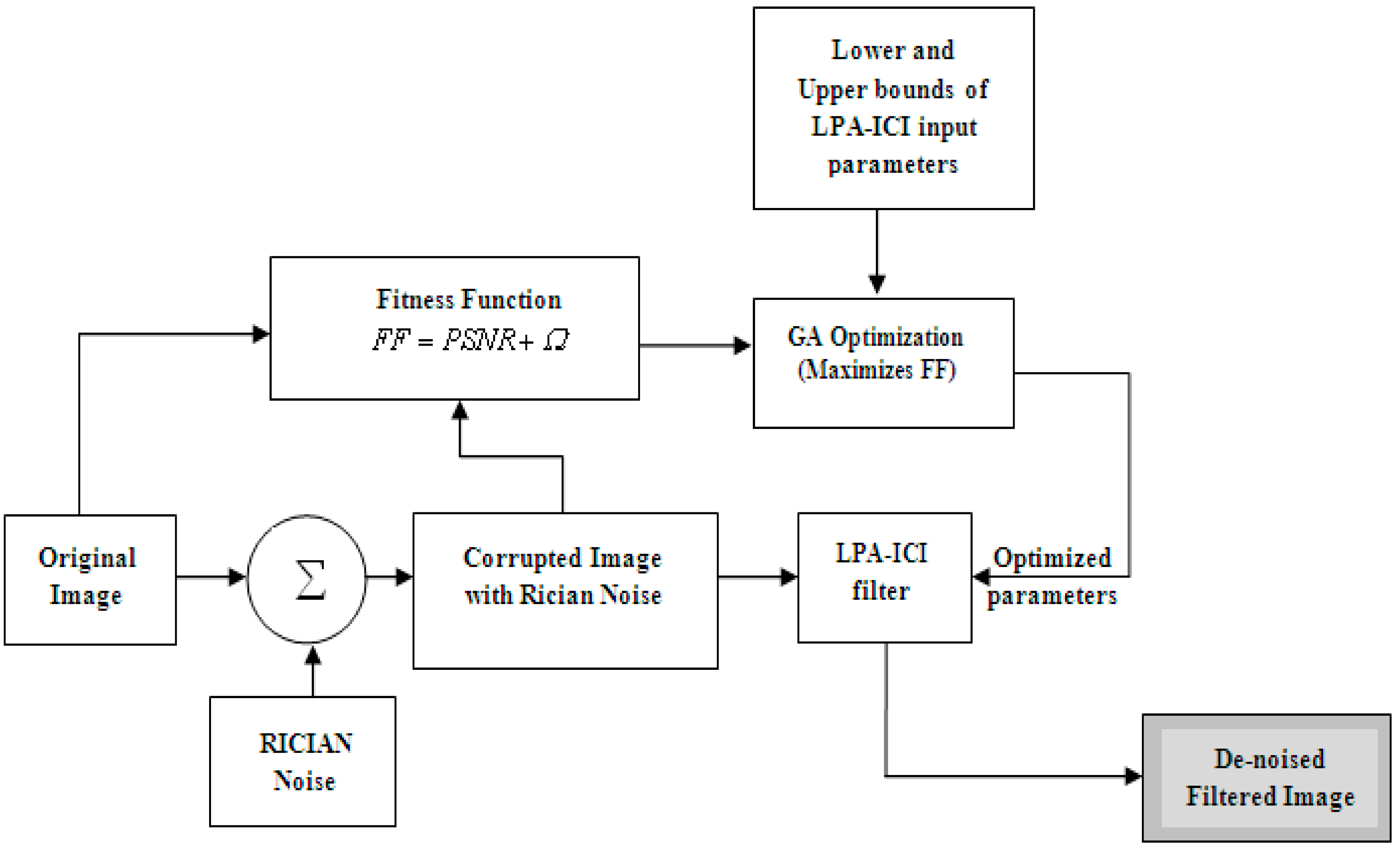
4. The Proposed LPA-GA System

Since, GA proves its efficiency for better convergence towards global optimization than any other global search algorithm. Consequently, the proposed method in this work makes use of genetic algorithm to determine the optimal parameter values in the LPA-ICI de-noising filter in order to reduce Rician noise by optimizing the mean square error taken as a cost function.

The brain tumor is a defined as a group of abnormal cells that grows inside of the brain or around the brain. Tumors can directly destroy all healthy brain cells. As well as it can indirectly damage healthy cells. The MRI is the main modality that concerned with brain images and other body parts. Thus, the brain images are used to test the proposed novel algorithm as the brain images considered as the second leading cause of cancer death.

The LPA-ICI-GA based filtering procedure maintains key image element and characteristics, reduces the Rician noise. In this paper, simulated Rician noise introduced in the test image slice and then the noise is filtered out using LPA-ICI based GA optimization.

Figure 1 depicts the proposed system using the following steps:

Step 1.   

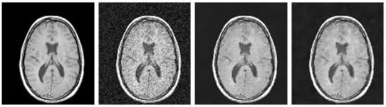
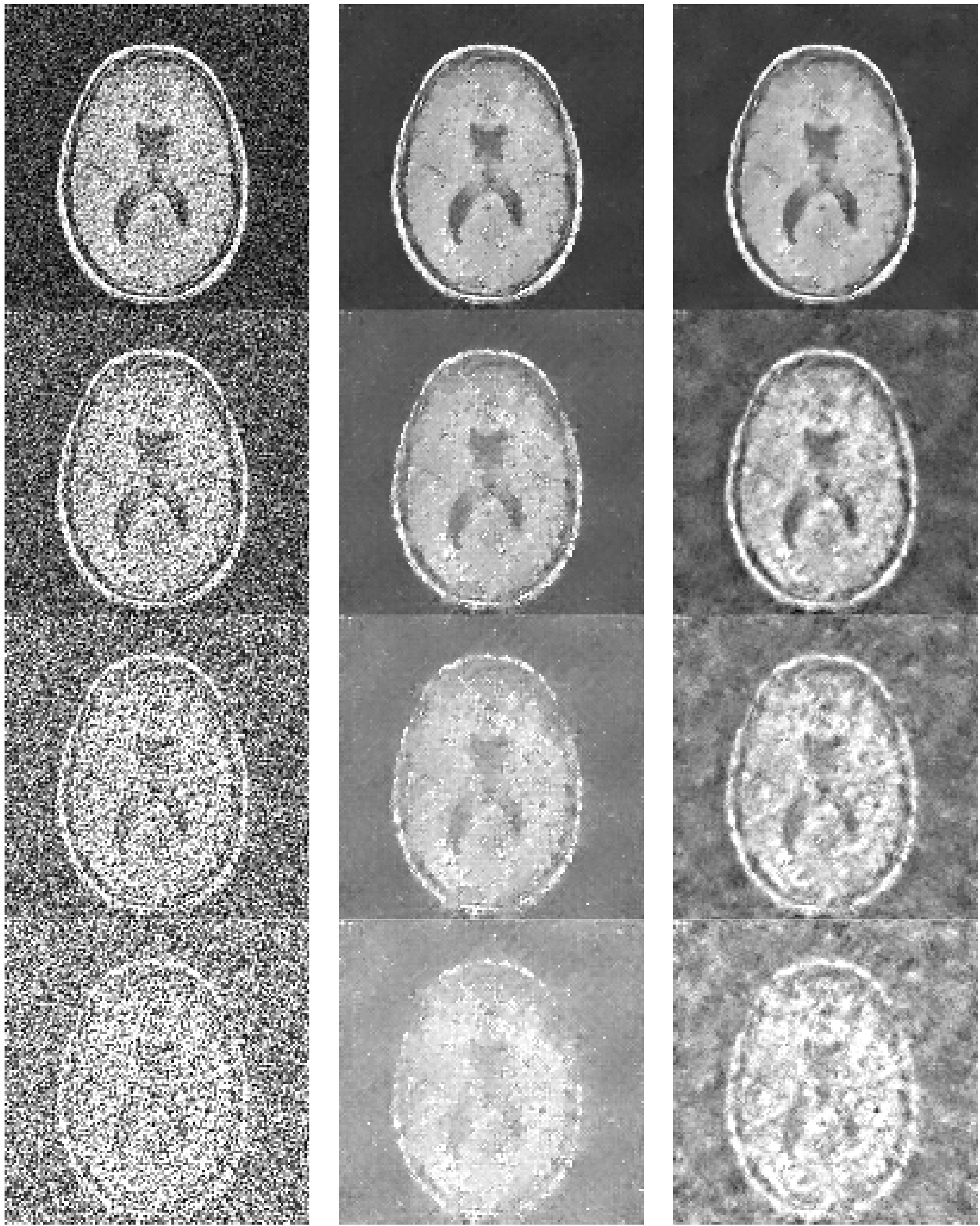
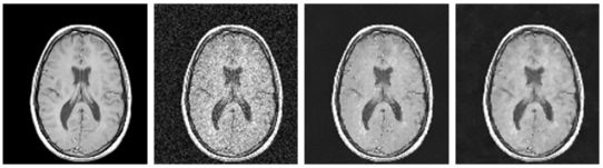
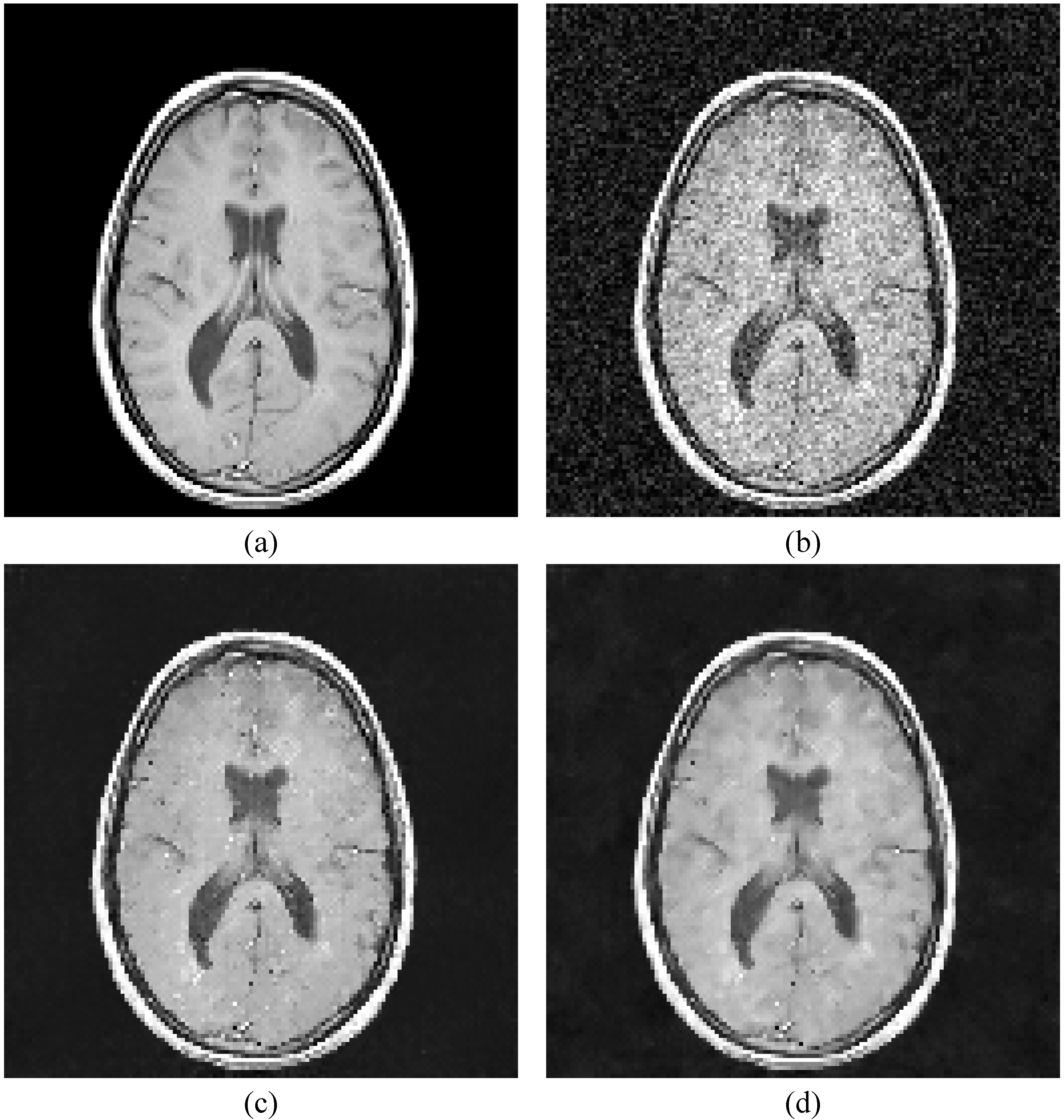
The original MRI-brain image is added with Rician noise with various values of “s” ranging from 0.1 to 0.6 to produce the corrupted images.

Step 2.   

The genetic algorithm is used to optimize the input parameters of LPA-ICI.

Step 3.   

The input parameters include the Gamma ICI parameter Γ, sharpness parameter, number of directions = 4 or 8, and fusion parameter which is classical or piecewise.

Step 4.   

The upper and lower bounds of the input parameters are set as [−1 to 10] for the Gamma ICI parameter, [0–5] for sharpness parameter, [[4 or 8] for direction parameter, [[1 or 2] for fusion parameter.

For each solution, the fitness function is to be computed based on the obtained PSNR and mean structural similarity (MSSIM) values. The solution set with the best fitness value is then selected and stored as the best solution for the gained parameters. The fitness function (FF) is calculated between the original and restored images, can be expressed as follows:

$$FF=PSNR+\Omega$$

(10)

where, Ω is the correlation factor defined as (Ω = 100* MSSIM). Here, the normal values of the MSSIM fall in the range 0~1; consequently, MSSIM are multiplied by 100, as the PSNR values may reach the value of 100.

Step 5.   

The fitness function uses the LPA-ICI with optimized parameters given by the GA to produce the restored image.

Step 6.   

The genetic algorithm is used to maximize the fitness function (by multiplying the result by −1). The number of generations is set to 100 by default.

Step 7.   

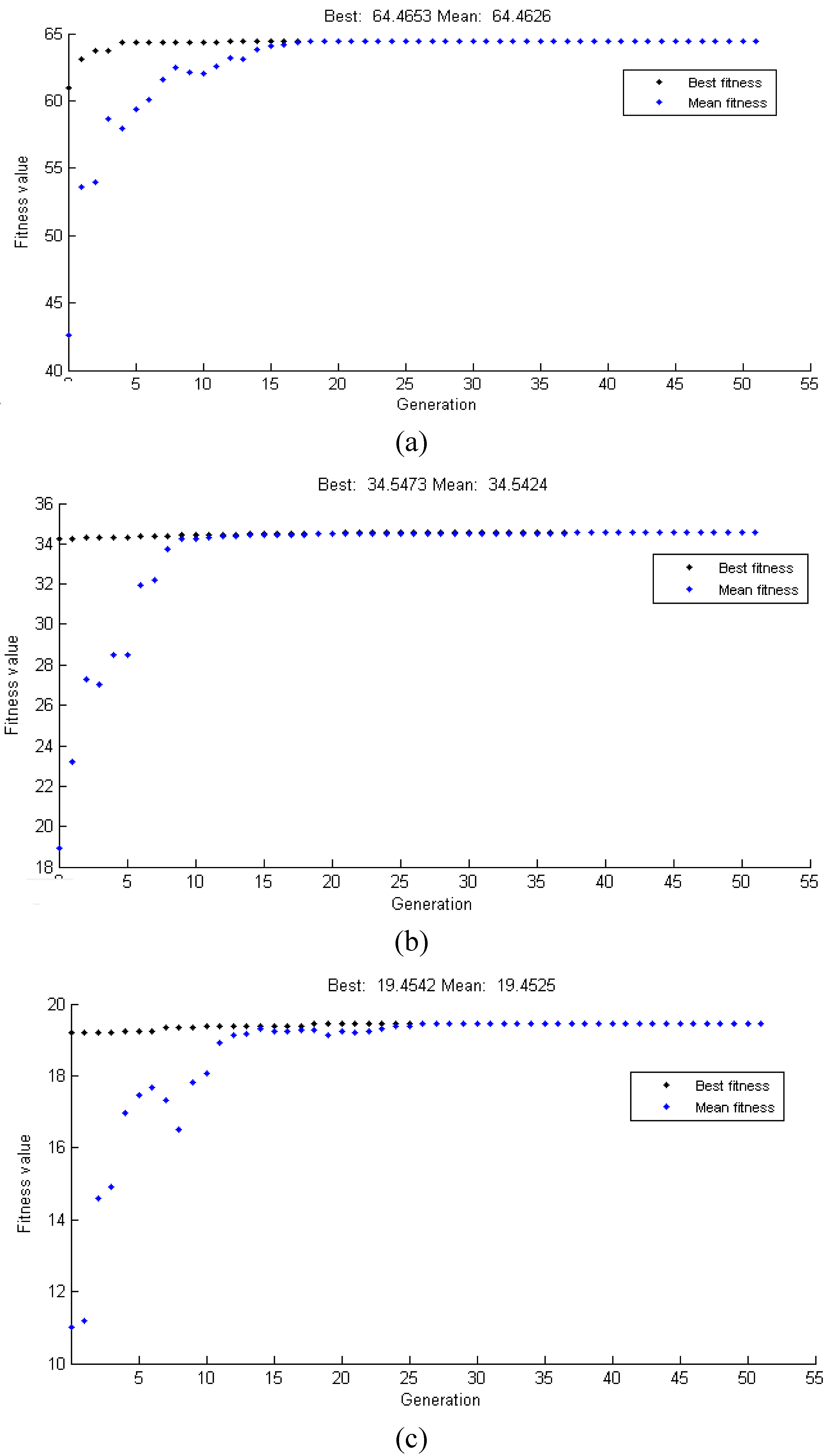
The genetic algorithm stopped around 50 generations for all noise ratios. Where, convergence occurred around 25 generations.

Step 8.   

The optimized parameters generated by the genetic algorithm are then given to the LPA-ICI filter to de-noise the corrupted image.

Step 9.   

The fitness function (FF), calculates PSNR+100*MSSIM between the original image and the restored image. Where, the LPA-ICI with parameters selected by GA is used to produce the restored image.

Figure 1. Proposed system block diagram.

Figure 1. Proposed system block diagram.

Through the GA stage, evaluation is executed via the fitness function which depends on the precise problem (de-noising) and is the optimization objective of the GA.

5. Result and Discussion

To study the local polynomial approximation based intersection confidence interval is supported by genetic algorithm for MRI brain images de-noising. The Matlab R2008a (Version 7.6.0.324) software is used. The algorithm has been executed at a base station in a Windows 7 platform having 6GB RAM, Intel Core i5-2410M CPU 2.30GHz processor. The experimental results are obtained using the public MRI data set of 27 horizontal slices of brain images, available at [67].

5.1. Comparing the results of LPA-ICI-GA versus LPA-ICI Algorithm

Figure 2 illustrates the results obtained from employing the LPA-ICI and the LPA-ICI-GA algorithms for de-noising the MRI brain slice images that corrupted with Rician noise of (s = 0.1) variance value. The figure demonstrates that the proposed system is able to restore the MRI image efficiently even with the existence of the Rician noise. Also, the image restored by LPA-ICI-GA is better than the restoration by LPA-ICI. It is clear that still some white dots are there when using LPA-ICI algorithm in Figure 2c. These results are shown when s = 0.1 where the proposed system provides perfect results for all noise variances less than 0.1.

Figure 2. Comparing the results of LPA-ICI-GA versus LPA-ICI algorithms for brain MRI slice restored images after adding Rician noise with s = 0.1 (noise variance). (a) is the Brain MRI original image, (b) Corrupted image with Rician noise with noise variance (s = 0.1), (c) is the de-noised image based LPA-ICI algorithm, and (d) is the de-noised image based LPA-ICI supported by the genetic algorithm (proposed system LPA-ICI-GA).

Figure 2. Comparing the results of LPA-ICI-GA versus LPA-ICI algorithms for brain MRI slice restored images after adding Rician noise with s = 0.1 (noise variance). (a) is the Brain MRI original image, (b) Corrupted image with Rician noise with noise variance (s = 0.1), (c) is the de-noised image based LPA-ICI algorithm, and (d) is the de-noised image based LPA-ICI supported by the genetic algorithm (proposed system LPA-ICI-GA).

Another comparison set of the brain MRI slice images is shown in Figure 3 for the same original image shown in Figure 2a after adding Rician noise with different variance levels. This figure shows a different comparison using the proposed (LPA-ICI-GA) and the LPA-ICI compared to the original brain MRI image after adding the Ricicn noise. The obtained results demonstrate the superiority of the proposed method over the LPA-ICI algorithm even with high noise variance values. At high noise variance, the images become not clear using LPA-ICI.

Figure 3. Comparing the results of LPA-ICI-GA versus LPA-ICI algorithms for brain MRI slice restored images after: (Left panel) adding Rician noise to the original image in Figure 2a at variance levels (s = 0.2, 0.3, 0.4, and 0.5, respectively); (Middle panel) restored images using LPA-ICI, (Right panel) restored images using LPA-ICI-GA.

Figure 3. Comparing the results of LPA-ICI-GA versus LPA-ICI algorithms for brain MRI slice restored images after: (Left panel) adding Rician noise to the original image in Figure 2a at variance levels (s = 0.2, 0.3, 0.4, and 0.5, respectively); (Middle panel) restored images using LPA-ICI, (Right panel) restored images using LPA-ICI-GA.

5.2. Proposed System Performance Analysis

Assume here that $Z\left(i,j\right)$ is the original image of siz $M_1\times M_2$, while $X\left(i,j\right)$ is the image restored using LPA-ICI with parameters given by the GA. Additionally, the fitness function (FF) is given by PSNR+100*MSSIM. To evaluate the system performance, various performance metrics are measured for both the proposed method (LPA-ICI-GA) and the LPA-ICI method. These metrics are SNR (Signal-to-Noise Ratio), PSNR (Peak SNR), ISNR (Improvement in SNR), MSE (Mean Squared Error), RMSE (Root of MSE), MAE (Mean Absolute Error), MAX (Maximum Absolute Difference). These metrics are defined as:

• Signal-to-noise ratio (SNR): is defined as the ratio of the power of the original image values and the power of noise values. It is given by:

  $$SNR=10\times {\log }_{10}\times \frac{{\displaystyle \sum {\displaystyle \sum X{(i,j)}^2}}}{{\displaystyle \sum {\displaystyle \sum {(Z(i,j)-X(i,j))}^2}}}$$

  (11)
• The improvement in signal to noise ratio (ISNR) between the original and restored images is given by:

  $$ISNR=10\times {\log }_{10}\times \frac{{\displaystyle \sum {\displaystyle \sum {\left(X\left(i,j\right)-Y\left(i,j\right)\right)}^2}}}{{\displaystyle \sum {\displaystyle \sum {\left(Z\left(i,j\right)-X\left(i,j\right)\right)}^2}}}$$

  (12)
• The peak signal to noise ratio (PSNR) between the original and restored images is given by [68]:

  $$PSNR=20\times {\log }_{10}\times \frac{255\times M\times N}{\sqrt{{\displaystyle \sum {\displaystyle \sum {\left(Z\left(i,j\right)-X\left(i,j\right)\right)}^2}}}}$$

  (13)
• The mean squared error (MSE): measures the average of the squares of the “errors”, known as the difference between the original image and the restored image. It is given by,

  $$MSE=\frac{{\displaystyle \sum {\displaystyle \sum {\left(Z\left(i,j\right)-X\left(i,j\right)\right)}^2}}}{M\times N}$$

  (14)
• The mean absolute error (MAE): is the average of the absolute errors between the original image and the restored image. It is given by:

  $$MAE=\frac{1}{M\times N}{\displaystyle \sum {\displaystyle \sum \left|Z\left(i,j\right)-X\left(i,j\right)\right|}}$$

  (15)
• The maximum absolute difference (MAD) is given by:

  $$MAD=\max \left(\left|Z\left(i,j\right)-X\left(i,j\right)\right|\right)$$

  (16)
• The SSIM index measure between two windows $Z$ and $X$ of the original and restored images is given by:

$$SSIM\left(x,z\right)=\frac{\left(2{\mu }_x{\mu }_z+C_1\right)\left(2{\sigma }_{xz}+C_2\right)}{\left({\mu }_x^2+{\mu }_z^2+C_1\right)\left({\sigma }_x^2+{\sigma }_z^2+C_2\right)}$$

(17)

where, ${\mu }_x$ is the average of X, ${\mu }_z$ is the average of Z, ${\sigma }_{x2}$ is the variance of X,${\sigma }_{z2}$is the variance of Z, ${\sigma }_{xz}$is the covariance of X and Z, $C_1={\left(K_{1}L\right)}^2$ and $C_2={\left(K_{2}L\right)}^2$ are two variables used to stabilize the division, L = 255 is the dynamic range of pixel-values, and $K_1$ = 0.01 and $K_2$ = 0.03 by default. The SSIM is calculated on various windows of the images.

• The mean structural similarity (MSSIM) index is given by:

$$MSSIM\left(X,Z\right)=\raisebox{1ex}{$1$}\!\left/ \!\raisebox{-1ex}{$P$}\right.{\displaystyle \sum _{J}SSIM\left(x_j,z_j\right)}$$

(18)

where, $x_j$ and $z_j$ are the image contents at the j^th local window, and P is the number of local windows in the image.

Along with these parameters with different Rician noise variance (s), the following results calculated.

Table 1 illustrates theses performance metrics when using the LPA-ICI without optimization; where the values used for the ICI parameters are fixed and are selected as to have the values: Sharpness parameter = −1, Γ = 1.05, Directional resolution = 8 and Fusing = 1 [65], at different values of the noise variance “s”. Where these parameters are set to be fixed when using the LPA based ICI rule, then adjust the window size according to theses fixed value parameters which affect its performance. Where, the LPA-ICI multi-directional kernels give additional enhancement, providing an efficient tool especially for image de-noising, differentiation and inverse-imaging problems.

Table 1. The performance metrics values for the LPA-ICI without GA.

S	ISNR	SNR	PSNR	MSE	RMSE	MAE	MAX	MSSIM
0.1	1.55	12.2267	19.5451	722.0499	26.871	23.7222	95.379	0.44208
0.2	1.6386	6.31	13.6284	2819.9239	53.103	46.5034	190.9031	0.31629
0.3	1.6375	2.8197	10.1381	6299.0275	79.3664	69.6002	245.642	0.22051
0.4	1.612	0.31846	7.6369	11204.5665	105.8516	93.8354	367.7877	0.15175
0.5	1.5691	-1.6638	5.6546	17685.5917	132.9872	119.8152	463.6092	0.10741
0.6	1.5325	-3.3066	4.0118	25816.7765	160.676	147.2261	559.6435	0.084966
0.7	1.4968	-4.718	2.6004	35730.901	89.0262	175.6339	655.8092	0.070399

Table 1. The performance metrics values for the LPA-ICI without GA.

S	ISNR	SNR	PSNR	MSE	RMSE	MAE	MAX	MSSIM
0.1	1.55	12.2267	19.5451	722.0499	26.871	23.7222	95.379	0.44208
0.2	1.6386	6.31	13.6284	2819.9239	53.103	46.5034	190.9031	0.31629
0.3	1.6375	2.8197	10.1381	6299.0275	79.3664	69.6002	245.642	0.22051
0.4	1.612	0.31846	7.6369	11204.5665	105.8516	93.8354	367.7877	0.15175
0.5	1.5691	-1.6638	5.6546	17685.5917	132.9872	119.8152	463.6092	0.10741
0.6	1.5325	-3.3066	4.0118	25816.7765	160.676	147.2261	559.6435	0.084966
0.7	1.4968	-4.718	2.6004	35730.901	89.0262	175.6339	655.8092	0.070399

The same metrics are measured for the same original test image used in Figure 2 and Figure 3 at different Rician noise variance “s”, when using the proposed LPA-ICI-GA that provides optimal parameter values that used in the ICI rule to determine the optimal window width. The optimal parameters values and the measured metrics are shown in Table 2 and Table 3.

Since, the proposed algorithm uses the genetic algorithm to optimize the ICI parameters, therefore a range for each parameter to be used. A Matlab Genetic Algorithm toolbox is used in the GA process. For these parameters tuning, selected random values for all the parameters in the integer numbers form are used as a combination set. It is noted that the authors in [65] test their algorithm for Γ range from 1.5 to 4.0. As, Γ is the threshold for the confidence interval used in the ICI rule to obtain the adaptive window size. Jointly with the fusing has only two possible values, where fusing = 1 for classical estimation, and equal 2 for piecewise estimation. In addition, the LPA-ICI uses the directional parameter to choose the number of directions in which the kernels will be applied. Actually, its range can be chosen to be integer from 1 to 8, but the most common values for the directional resolution are 4 and 8 neighborhood for a pixel. Generally, regarding the sharpening, −1 refers to “no sharpening”, and if greater than 0 refers to the “sharpening”, it multiplies the value with the kernel matrix to improve sharpness. Therefore, the parameter selection range will be:

• Sharpness parameter range = [−1, from 0 till 10];
• Γ range = [from 0 till 5];
• Directional resolution range = [[4 or 8];
• Fusing range = [[1 or 2], where Fusing = 1 for classical estimation, and equal 2 for piecewise estimation.

As clear from Table 2 and Table 3 that:

Step 1.   

According to the noise variance level, the ICI parameter optimal values are changeable. This proves the importance of the GA to obtain the optimized values for these parameters. Also, these parameter values are changeable with any change in the image concerned.

Step 2.   

The ICI tuned parameters (optimized), are different than the fixed values used in LPA-ICI. Also, as the noise variance increase and equal 0.6 both fusing and the directional resolution switches their values, to be able to overcome the high noise level.

Step 3.   

Comparing the performance metrics values in Table 1 and Table 3, it is clear that, the proposed method is outperforming the LPA-ICI in terms of all the metric values.

Table 2. The optimal ICI parameter values when using LPA-ICI-GA for MRI image de-noising.

S	SharpParam	Γ	Directional Resolution	Fusing
0.1	−0.4495	0.4984	8	2
0.2	−0.7464	0.7165	8	2
0.3	0.0126	0.6696	8	2
0.4	−0.1287	0.5449	8	2
0.5	−0.0556	0.5540	8	2
0.6	−0.2439	0.5234	8	2
0.7	−0.8946	2.3293	4	1

Table 2. The optimal ICI parameter values when using LPA-ICI-GA for MRI image de-noising.

S	SharpParam	Γ	Directional Resolution	Fusing
0.1	−0.4495	0.4984	8	2
0.2	−0.7464	0.7165	8	2
0.3	0.0126	0.6696	8	2
0.4	−0.1287	0.5449	8	2
0.5	−0.0556	0.5540	8	2
0.6	−0.2439	0.5234	8	2
0.7	−0.8946	2.3293	4	1

Table 3. The performance metrics values when using LPA-ICI-GA for MRI image de-noising.

S	ISNR	SNR	PSNR	MSE	RMSE	MAE	MAX	MSSIM	Fitness Function = PSNR+100*MSSIM
0.1	1.5982	12.275	19.5934	714.0724	26.7221	23.4761	95.379	0.44871	64.4645
0.2	1.6994	6.3708	13.6892	2780.722	52.7325	45.9734	190.9031	0.32608	46.2971
0.3	1.8495	3.0317	10.3501	5998.932	77.4528	68.2574	211.127	0.24197	34.5472
0.4	1.822	0.52845	7.8469	10,675.67	103.3231	91.4624	238.5945	0.18155	26.0015
0.5	1.7566	−1.4763	5.8421	1,6938.2	130.1469	116.3874	297.4721	0.13606	19.4483
0.6	1.6849	−3.1542	4.1642	2,4926.53	157.8814	143.7663	312.2485	0.10795	14.9587
0.7	1.4848	−4.73	2.5884	3,5829.55	189.2869	176.1798	363.922	0.085832	11.1716

Table 3. The performance metrics values when using LPA-ICI-GA for MRI image de-noising.

S	ISNR	SNR	PSNR	MSE	RMSE	MAE	MAX	MSSIM	Fitness Function = PSNR+100*MSSIM
0.1	1.5982	12.275	19.5934	714.0724	26.7221	23.4761	95.379	0.44871	64.4645
0.2	1.6994	6.3708	13.6892	2780.722	52.7325	45.9734	190.9031	0.32608	46.2971
0.3	1.8495	3.0317	10.3501	5998.932	77.4528	68.2574	211.127	0.24197	34.5472
0.4	1.822	0.52845	7.8469	10,675.67	103.3231	91.4624	238.5945	0.18155	26.0015
0.5	1.7566	−1.4763	5.8421	1,6938.2	130.1469	116.3874	297.4721	0.13606	19.4483
0.6	1.6849	−3.1542	4.1642	2,4926.53	157.8814	143.7663	312.2485	0.10795	14.9587
0.7	1.4848	−4.73	2.5884	3,5829.55	189.2869	176.1798	363.922	0.085832	11.1716

5.3. Proposed System Convergence Graphs

Figure 4 is related to Table 2 as it shows the obtained convergence graph where the graph reports the number of iterations (generations) versus the fitness function when using the GA. It is obvious from Figure 4 that, as the noise variance level increase, the fitness function value decreases. Also, the range of number of generations (iterations) required for convergence is about 25 iterations maximum and it varies according to the noise variance value.

Figure 4. The fitness-convergence graph at different noise variance values (s= (a) 0.1, (b) 0.3 and (c) 0.5).

Figure 4. The fitness-convergence graph at different noise variance values (s= (a) 0.1, (b) 0.3 and (c) 0.5).

In literature [69] by Iftikhar et al., similar work has been done in recent past. The authors employed Elite GA (EGA) to find the optimal values that the Non-local means (NLM) filter depends on the patch size, search window size and the smoothing parameters. It was reported that for given images, the GA converges well before 50 iterations using the PSNR as fitness value. While, using the EGA accelerate the search process with better convergence rate. The authors tested images of different noise level variance (10, 15 and 20). For synthetic images, it was stated that at variance = 10, the GA converged at 32 iterations while the EGA converged at 26 iterations. While, with variance = 15 or 20, both the GA and EGA converged at 21 iterations. With respect to the PSNR the GA and EGA recorded the same 35.87, 32.80, and 31.67 for variance values of 10, 15, and 20; respectively. Moreover, with respect to the RMSE both algorithms reported the same values which were 3.77, 5.28, and 6.29 for variance values of 10, 15, and 20; respectively.

Where as in our work using LPA-ICI-GA algorithm, the variance level was in the range from 0.1 to 0.7, where the LPA-ICI-GA algorithm converged after about 25 iterations. As established by Table 3, the PSNR equal 19.5934, 13.6892, and 10.3501 with s = 0.1, 0.2, and 0.3; respectively. Furthermore, the RMSE had values of 26.7221, 52.7325, and 77.4528 with s = 0.1, 0.2, and 0.3; respectively.

Comparing the results obtained by our proposed algorithm to that obtained by Iftikhar et al. [69]. It is clear that, even if the dataset, variance level, and fitness function are different in Iftikhar et al. [69] from those used in the current proposed technique, it can be concluded that our obtained results are very much encouraging and promising.

Moreover, a lot of work has been done in recent time in the area of MRI de-noising. The following table (Table 4) shows some of these related methods indicating the de-noising techniques used and compared to the proposed method.

It is clear from Table 4 that, most of the work in the literature were used conventional de-noising techniques, while the selection of any filter parameters are considered an optimization problem. In this work the main motivation is to use optimization algorithm to adjust the parameters of the classic LPA-ICI filter, i.e., the optimal window size selection, for MRI images de-noising. Thus, the GA optimization approach is used in order to reduce the Rician noise by optimizing the mean square error taken as a cost function. The main contribution of this work can be pointed as: (I) used GA for optimal window size selection for the classic LPA-ICI, (II) provided the optimal window size with changeable image under concern, (III) compared the performance metrics’ values of the proposed system to those for the classic LPA-ICI system, (IV) proved that the proposed method is outperforming the LPA-ICI in terms of all the metric values, (V) tested the proposed novel idea with different Rician noise variance levels, (VI) used the brain MRI images corrupted with Rician noise to test the proposed system, (VII) achieved about 25 iteration maximum for convergence and it varies according to the noise variance value, (IX) established the superior efficiency of the proposed LPA-ICI-GA over the classic LPA-ICI for MRI images de-noising, (X) for variance of 0.1, the PSNR using the proposed method is 19.5934 dB, while that obtained by the LPA-ICI was 19.5451. Comparing with respect to the MSE at the same variance value, it was obtained that the LPA-ICI-GA compared to the LPA-ICI achieved 714.0724 and 722.0499; respectively. That established that the proposed method gained less MSE compared to the classical LPA-ICI approach, and (XI) endowed with a high level of noise reduction, it can give good performance till noise variance level of 0.5.

Table 4. Comparison table of related work for MRI images de-noising and the current study.

S. No.	Authors	Year	De-Noising Technique	Comments/Notes
1	Bao et al. [15]	2003	Adaptive wavelet thresholding	To, this method multiplied the adjacent wavelet sub bands, then applied threshold to the multi-scale products to differentiate edge structures in an improved approach from noise and amplify the significant features. Results of MRI images proved that this method achieved high mean-to-standard-deviation ratio (MSR) and contrast to noise ratio (CNR).
2	Wang et al. [18]	2006	Wavelet and the total variation minimization methods	An effective automatic stopping time criterion extensively.
3	Manjon et al. [19]	2009	Novel filter averaging similar patches around the image using a robust multicomponent similarity measure filter, then local Principal Component Analysis decomposition as a post-processing for more noise removal.	This method showed a consistent improvement in the results when the number of images increases in contrast with the erratic behavior of the basic version.
4	Jaya et al. [23]	2009	Median filter, the weighted median and the adaptive filter.	The results proved that weighted median filter was outperforming the other filters with peak signal to noise ratio PSNR = 0.924.
5	Rajeesh et al. [20]	2010	Curvelet shrinkages were superior than using the wavelet method.	The reconstructed MRI data have high Signal to Noise Ratio (SNR) compared to the curvelet and wavelet domain denoising approaches.
6	Erturk et al. [22]	2013	Spectral subtraction method.	The results showed enhanced signal to noise ratio (SNR) up to 40% in the MRI reconstructed signal
7	Proposed system	2015	Local polynomial approximation with intersection confidence interval based genetic algorithm filter. (LPA-ICI-GA)	The results proved that using GA optimization to support the LPA-ICI outperform the classic LPA-ICI. For variance of 0.1, the PSNR using the proposed method is 19.5934 dB, while that obtained by the LPA-ICI was 19.5451. Comparing with respect to the MSE at the same variance value, it was obtained that the LPA-ICI-GA compared to the LPA-ICI achieved 714.0724 and 722.0499; respectively. That established that the proposed method gained les MSE compared to the classical LPA-ICI approach.

Table 4. Comparison table of related work for MRI images de-noising and the current study.

S. No.	Authors	Year	De-Noising Technique	Comments/Notes
1	Bao et al. [15]	2003	Adaptive wavelet thresholding	To, this method multiplied the adjacent wavelet sub bands, then applied threshold to the multi-scale products to differentiate edge structures in an improved approach from noise and amplify the significant features. Results of MRI images proved that this method achieved high mean-to-standard-deviation ratio (MSR) and contrast to noise ratio (CNR).
2	Wang et al. [18]	2006	Wavelet and the total variation minimization methods	An effective automatic stopping time criterion extensively.
3	Manjon et al. [19]	2009	Novel filter averaging similar patches around the image using a robust multicomponent similarity measure filter, then local Principal Component Analysis decomposition as a post-processing for more noise removal.	This method showed a consistent improvement in the results when the number of images increases in contrast with the erratic behavior of the basic version.
4	Jaya et al. [23]	2009	Median filter, the weighted median and the adaptive filter.	The results proved that weighted median filter was outperforming the other filters with peak signal to noise ratio PSNR = 0.924.
5	Rajeesh et al. [20]	2010	Curvelet shrinkages were superior than using the wavelet method.	The reconstructed MRI data have high Signal to Noise Ratio (SNR) compared to the curvelet and wavelet domain denoising approaches.
6	Erturk et al. [22]	2013	Spectral subtraction method.	The results showed enhanced signal to noise ratio (SNR) up to 40% in the MRI reconstructed signal
7	Proposed system	2015	Local polynomial approximation with intersection confidence interval based genetic algorithm filter. (LPA-ICI-GA)	The results proved that using GA optimization to support the LPA-ICI outperform the classic LPA-ICI. For variance of 0.1, the PSNR using the proposed method is 19.5934 dB, while that obtained by the LPA-ICI was 19.5451. Comparing with respect to the MSE at the same variance value, it was obtained that the LPA-ICI-GA compared to the LPA-ICI achieved 714.0724 and 722.0499; respectively. That established that the proposed method gained les MSE compared to the classical LPA-ICI approach.

Due to the efficient performance of the proposed system, it can be generalized to be used with any type of medical/ non-medical images for de-noising and restore the images.

6. Conclusions and Future work

Noise is a significant factor that can maneuver medical image quality. Medical images are vulnerable to noise affect in the process of transmission and processing which cause the loss of image contrast, blur, etc. Physicians will not be able to discriminate the interested lesions, thus influence the diagnosis, when the diseased tissue and normal tissue attenuation coefficient is very small. So, filtering out the signal noise, getting a restored noise free image, become the physician’s main concern. In recent year, Medical image de-noising is an evolving research area that has obtained vast consideration among the researchers. Significant researches and techniques that exist for medical image de-noising are pursued.

Due to the nonparametric characteristic of the local polynomial approximation filter and the frequency distribution characteristics of noise, LPA-ICI had a superior benefit in image de-noising. In this work to improve this method an optimization algorithm is to be used to optimize the ICI parameters that used later to determine the sliding window size. Since, the Genetic Algorithm uses a bulky number of solutions, rather than a single solution for searching. So, GA is a robust procedure that improves the chance of realizing the global optimum and nearly unbiased optimization techniques for sampling a large solution space. Thus, the GA is used to support the LPA-ICI de-noising filter.

This proposed method is tested using brain MRI images corrupted with Rician noise. Where, MRI has developed appreciably over the last few decades. It is commonly well recognized to model noise on magnitude MR images as white and Rician distributed.

An innovative approach to de-noise Rician noise has been conducted in this work which use of the Genetic Algorithm to optimize the ICI parameters using a fitness function. The GA proves its efficiency in this proposed method as it achieves better results, fast processing times and easy implementation with satisfactory performance compared to using LPA-ICI without optimization. In addition to, the proposed method endowed with a high level of noise reduction, it can give good performance till noise variance level of 0.5.Current work reports better PSNR, ISNR, SNR, MSE, MAE, and MAX values.

For further work, it is suggested to change the parameters range used study its effect on the proposed method. For example, it is possible to check if the Directional resolution range has other values rather than 4 and 8 only.

Furthermore, it is suggested to compare the proposed method performance with that obtained using wavelet and wavelet based GA and compares the computed time efficiency. In addition, the proposed algorithm can be tested with any other medical image modalities. Besides, it is recommended to use different optimization algorithms either heuristic or meta-heuristic and compare their performance when used with the LPA-ICI or RICI de-noising filters.

References

1. Dey, N.; Das, P.; Roy, A.; Das, A.; Chaudhuri, S. Detection and measurement of Arc of Lumen calcification from intravascular ultrasound using Harris corner detection. In Proceedings of National Conference on Computing and Communication Systems (NCCCS), Durgapur, India, 21–22 November 2012.
2. Dey, N.; Roy, A.; Pal, M.; Das, A. FCM based blood vessel segmentation method for retinal images. Int. J. Comput. Sci. Netw. 2012, 1. [Google Scholar]
3. Araki, T.; Ikeda, N.; Molinari, F.; Dey, N.; Acharjee, S.; Saba, L.; Nicolaides, A.; Suri, J. Effect of geometric-based coronary calcium volume as a feature along with its shape-based attributes for cardiological risk prediction from low contrast IVUS. J. Med. Imaging Health Inform. 2014, 4, 255–261. [Google Scholar] [CrossRef]
4. Dey, N.; Dey, M.; Biswas, D.; Das, P.; Das, A.; Chaudhuri, S. Tamper detection of electrocardiographic signal using watermarked bio-hash code in wireless cardiology. Int. J. Signal Imaging Syst. Eng. 2015, 8, 46–58. [Google Scholar] [CrossRef]
5. Bilcu, R.; Vehvilainen, M. A novel decomposition scheme for image de-noising. In Proceedings of the IEEE International Conference on Acoustics, Speech and Signal Processing, Honolulu, HI, USA, 15–20 April 2007; pp. 577–580.
6. Alpuente, L.; López, A.; Tur, R. Glioblastoma: Changing expectations? Clin. Trans. Oncol. 2011, 13, 240–248. [Google Scholar] [CrossRef] [PubMed]
7. Sijbers, J.; Dekker, A.; Audekerke, J.; Verhoye, M.; Dyck, D. Estimation of the noise in magnitude MR images. Magn. Reson. Imaging 1998, 16, 87–90. [Google Scholar] [CrossRef]
8. Rice, S. Mathematical analysis of random noise. Bell Syst. Tech. J. 1944, 23, 282–332. [Google Scholar] [CrossRef]
9. Ali, S.; Vathsal, S.; Lalkishore, K. A GA-based window selection methodology to enhance window-based multi-wavelet transformation and thresholding aided CT image denoising technique. Int. J. Comput. Sci. Inf. Secur. 2010, 7. [Google Scholar]
10. Ali, S.A.; Vathsal, S.; Kishore, K.L. CT image denoising technique using GA aided window based multiwavelet transformation and thresholding with the incorporation of an effective quality enhancement method. Int. J. Digit. Content Technol. Appl. 2010, 4, 75–87. [Google Scholar]
11. Dey, N.; Das, A.; Chaudhuri, S. Wavelet based normal and abnormal heart sound identification using spectrogram analysis. Int. J. Comput. Sci. Eng. Technol. 2012, 3, 186–192. [Google Scholar]
12. Dey, N.; Roy, A.; Das, A.; Chaudhuri, S. Stationary wavelet transformation based self-recovery of blind-watermark from electrocardiogram signal in the wireless telecardiology. In Proceedings of the International Workshop on Intelligence and Security Informatics for International Security (IIS’12), Trivandrum, India, 11–12 October 2012.
13. Healy, D.; Weaver, J. Two applications of wavelet transforms in magnetic resonance imaging. IEEE Trans. Inf. Theory 1992, 38, 840–860. [Google Scholar] [CrossRef]
14. Nowak, R. Wavelet-based Rician noise removal for magnetic resonance imaging. IEEE Trans. Image Process. 1999, 8, 1408–1419. [Google Scholar] [CrossRef] [PubMed]
15. Bao, P.; Zhang, L. Noise reduction for magnetic resonance images via adaptive multiscale products thresholding. IEEE Trans. Med. Imaging 2003, 22, 1089–1099. [Google Scholar] [CrossRef] [PubMed]
16. Jiang, L.; Yang, W. Adaptive magnetic resonance image denoising using mixture model and wavelet shrinkage. In Proceeding of the VIIth Digital Image Computing: Techniques and Applications, Sydney, Australia, 10–12 December 2003; pp. 831–838.
17. Kadah, Y. Adaptive denoising of event-related functional magnetic resonance imaging data using spectral subtraction. IEEE Trans. Biomed. Eng. 2004, 51, 1944–1953. [Google Scholar] [CrossRef] [PubMed]
18. Wang, Y.; Zhou, H. Total variation wavelet-based medical image denoising. Int. J. Biomed. Imaging 2006, 2006. Article ID 89095. [Google Scholar]
19. Manjon, J.; Thacke, N.; Lull, J.; Mar, G.; Bonmat, L.; Robles, M. Research article multicomponent MR image denoising. Int. J. Biomed. Imaging 2009, 2009, 1–10. [Google Scholar] [CrossRef] [PubMed]
20. Rajeesh, J.; Moni, R.; Palanikumar, S.; Gopalakrishnan, T. Noise reduction in magnetic resonance images using wave atom shrinkage. Int. J. Image Process. 2010, 4, 131–141. [Google Scholar]
21. Balafar, M. Review of noise reducing algorithms for brain MRI images. Int. J. Tech. Phys. Probl. Eng. 2012, 4, 54–59. [Google Scholar]
22. Erturk, M.; Bottomley, P.; El-Sharkawy, A. Denoising MRI using spectral subtraction. IEEE Trans. Biomed. Eng. 2013, 60, 1556–1562. [Google Scholar] [CrossRef] [PubMed]
23. Jaya, J.; Thanushkodi, K.; Karnan, M. Tracking algorithm for de-noising of MR brain images. Int. J. Comput. Sci. Netw. Secur. 2009, 9, 262–267. [Google Scholar]
24. Iftikhar, M.A.; Jalil, A.; Rathore, S.; Ali, A.; Hussain, M. Brain MRI denoizing and segmentation based on improved adaptive nonlocal means. Int. J. Imaging Syst. Technol. 2013, 23, 235–248. [Google Scholar] [CrossRef]
25. Jalil, A.; Rathore, S.; Hussain, M. Robust brain MRI denoising and segmentation using enhanced non-local means algorithm. Int. J. Imaging Syst. Technol. 2014, 24, 52–66. [Google Scholar]
26. Iftikhar, M.A.; Jalil, A.; Rathore, S.; Ali, A.; Hussain, M. An extended non-local means algorithm: Application to brain MRI. Int. J. Imaging Syst. Technol. 2014, 24, 293–305. [Google Scholar] [CrossRef]
27. Klepaczko, A. AGPU Accelerated Local Polynomial Approximation Algorithm for Efficient Denoising of MR Images; Burduk, R., Jackowski, K., Kurzynski, M., Wozniak, M., Zolnierek, A., Eds.; Springer International Publishing: Cham, Switzerland, 2013. [Google Scholar]
28. Coupé, P.; Manjón, J.; Gedamu, E.; Arnold, D.; Robles, M.; Collins, D.L. Robust Rician noise estimation for MR images. Med. Image Anal. 2010, 14, 483–493. [Google Scholar] [CrossRef] [PubMed]
29. Tan, X.; Sun, C.; Pham, T.D. Multipoint filtering with local polynomial approximation and range guidance. In Proceeding of the 2014 IEEE Conference in Computer Vision and Pattern Recognition (CVPR), Columbus, OH, USA, 23–28 June 2014; pp. 2941–2948.
30. Hu, Y.; Jiang, X.; Xin, F.; Zhang, T.; Yuan, J.; Zhai, L.; Guo, C. An algorithm on processing medical image based on rough-set and genetic algorithm. In Proceedings of the International Conference on Information Technology and Applications in Biomedicine, Shenzhen, China, 30–31 May 2008.
31. Samanta, S.; Dey, N.; Das, P.; Acharjee, S.; Chaudhuri, S. Multilevel threshold based gray scale image segmentation using Cuckoo search. In Proceedings of the International Conference on Emerging Trends in Electrical, Communication and Information Technologies (ICECIT), Anantapur, India, 12–23 December 2012.
32. Chakraborty, S.; Pal, A.; Dey, N.; Das, D.; Acharjee, S. Foliage area computation using Monarch butterfly algorithm. In Proceedings of the 2014 1st International Conference on Non Conventional Energy, Kalyani, India, 16–17 January 2014.
33. Jayashri, P.; Gandhimathi, D. Efficient tumor segmentation in medical images using artificial bee colony optimization algorithm and fuzzy c-means clustering. Int. J. Adv. Res. Comput. Sci. Manag. Stud. 2014, 2, 98–101. [Google Scholar]
34. Acharjee, S.; Dey, N.; Samanta, S.; Das, D.; Roy, R.; Chakraborty, S.; Chaudhuri, S. ECG signal compression using ant weight lifting algorithm for tele-monitoring. J. Med. Imaging Health Inform. 2014, 5, 1580–1587. [Google Scholar]
35. Day, N.; Samanta, S.; Chakraborty, S.; Das, A.; Chaudhuri, S.; Suri, J. Firefly algorithm for optimization of scaling factors during embedding of manifold medical information: An application in ophthalmology imaging. J. Med. Imaging Health Inform. 2014, 4, 384–394. [Google Scholar] [CrossRef]
36. Misra, D.; Sarker, S.; Dhabal, S.; Ganguly, A. Effect of using genetic algorithm to denoise MRI images corrupted with Rician Noise. In Proceedings of the 2013 IEEE International Conference on Emerging Trends in Computing, Communication and Nanotechnology, Tirunelveli, India, 25–26 March 2013; pp. 146–151.
37. Liu, Y.; Ma, Y.; Liu, F.; Zhang, X.; Yang, Y. The research based on the genetic algorithm of wavelet image denoising threshold of medicine. J. Chem. Pharm. Res. 2014, 6, 2458–2462. [Google Scholar]
38. Tsang, P.; Au, A. A genetic algorithm for projective invariant object recognition. In Proceedings of the 1996 IEEE TENCON: Digital Signal Processing Applications, Perth, WA, USA, 26–29 November 1996; pp. 58–63.
39. Yang, J.; Fan, J.; Ai, D.; Zhou, S.; Tang, S.; Wang, Y. Brain MR image denoising for Rician noise using pre-smooth non-local means filter. Biomed. Eng. Online 2015, 14, 1–20. [Google Scholar] [CrossRef] [PubMed]
40. Gudbjartsson, H.; Patz, S. The Rician distribution of noisy MRI data. Magn. Reson. Med. 1995, 34, 910–914. [Google Scholar] [CrossRef] [PubMed]
41. Jagadeesan, H.; Sasirekha, N. Robust Rician noise estimation and filtering for magnetic resonance imaging. Int. J. Sci. Eng. Res. 2014, 5, 620–624. [Google Scholar]
42. Selvathi, D.; Selvi, S.; Malar, C. The SURE-LET approach for MR brain image denoising using different shrinkage rules. Int. J. Healthc. Inf. Syst. Inform. 2010, 5, 73–81. [Google Scholar] [CrossRef]
43. Edelstein, W.; Glover, G.; Hardy, C.; Redington, R. The intrinistic signal-to-noise ratio in MR imaging. Magn. Reson. Med. 1986, 3, 604–618. [Google Scholar] [CrossRef] [PubMed]
44. Macovski, A. Noise in MRI. Magn. Reson. Med. 1996, 36, 494–497. [Google Scholar] [CrossRef] [PubMed]
45. Basu, S.; Fletcher, T.; Whitaker, R. Rician noise removal in diffusion tensor MRI. In Medical Image Computing and Computer-Assisted Intervention—MICCAI 2006; Larsen, R., Nielsen, M., Sporring, J., Eds.; Springer: Berlin, Germany, 2006; pp. 117–125. [Google Scholar]
46. Papoulis, A. Probability, Random Variables, and Stochastic Processes; McGraw-Hill: New York, NY, USA, 1984. [Google Scholar]
47. Nobi, M.; Yousuf, M. A new method to remove noise in magnetic resonance and ultrasound images. J. Sci. Res. 2011, 3, 81–89. [Google Scholar]
48. Lee, J.S. Digital image enhancement and noise filtering by use of local statistics. IEEE Trans. Pattern Anal. Mach. Intell. 1980, 2, 165–168. [Google Scholar] [CrossRef] [PubMed]
49. Russ, J. The Image Processing Handbook, 6th ed.; CRC Press: Baca Raton, FL, USA, 1999. [Google Scholar]
50. Lee, Y.; Rhee, S. Wavelet-based image denoising with optimal filter. Int. J. Inf. Process. Syst. 2005, 1, 32–35. [Google Scholar]
51. Gupta, V.; Mahle, R.; Shriwas, R.S. Image denoising using wavelet transform method. In Proceedings of the 2013 Tenth International Conference on Wireless and Optical Communications Networks (WOCN), Bhopal, India, 26–28 July 2013.
52. Weaver, D.; Xu, Y.; Driscoll, J. Filtering MR images in the wavelet transform domain. Magn. Reson. Med. 1991, 21, 288–295. [Google Scholar] [CrossRef] [PubMed]
53. Hilton, M.; Ogden, T.; Hattery, D.; Eden, G.; Jawerth, B. Wavelet de-noising of functional MRI data. In Wavelets in Biology and Medicine; Aldroubi, A., Unser, M., Eds.; CRC Press: Baca Raton, FL, USA, 1996; pp. 93–112. [Google Scholar]
54. Piˇzurica, A.; Philips, W.; Lemahieu, I.; Acheroy, M. A versatile wavelet domain noise filtration technique for medical imaging. IEEE Trans. Med. Imaging 2003, 22, 323–331. [Google Scholar] [CrossRef] [PubMed]
55. Katkovnik, V. A new method for varying adaptive bandwidth selection. IEEE Trans. Signal Process. 1999, 47, 2567–2571. [Google Scholar] [CrossRef]
56. Ashour, A.; Elkamchouchi, H. Enhancement of moving targets tracking performance using the ICI rule. Alex. Eng. J. 2007, 46, 673–682. [Google Scholar]
57. Perona, P.; Malik, J. Scale-space and edge detection using anisotropic diffusion. IEEE Trans. PAMI 1990, 12, 629–639. [Google Scholar] [CrossRef]
58. Li, S.; Huang, D. Image denoising using non-negative sparse coding shrinkage algorithm. In Proceedings of the IEEE Computer Society Conference on Computer Vision and Pattern Recognition, San Diego, CA, USA, 20–25 June 2005; pp. 1017–1022.
59. Crouse, M.; Nowak, R.; Baraniuk, R. Wavelet-based statistical signal processing using hidden markov models. IEEE Trans. Signal Process. 1998, 46, 886–902. [Google Scholar] [CrossRef]
60. Jangra, S.; Yadav, S. A review of Rician noise reduction in MRI images using wave atom transform. Int. J. Comput. Sci. Mob. Comput. 2014, 3, 454–457. [Google Scholar]
61. Katkovnik, V.; Egiazarian, K.; Astola, J. Local Approximation Techniques in Signal and Image Processing; SPIE Press: Bellingham, WA, USA, 2006. [Google Scholar]
62. Katkovnik, V.; Egiazarian, K.; Astola, J. A spatially adaptive nonparametric regression image deblurring. IEEE Trans. Image Process. 2005, 14, 1469–1478. [Google Scholar] [CrossRef] [PubMed]
63. Fan, J.; Gijbels, I. Local Polynomial Modelling and Its Application; Chapman and Hall: London, UK, 1996. [Google Scholar]
64. Katkovnik, V. The Method of Local Approximation; Nauka: Moscow, Russia, 1985. [Google Scholar]
65. Katkovnik, V.; Egiazarian, K.; Astola, J. Adaptive window size image de-noising based on Intersection of Confidence Intervals (ICI) rule. J. Math. Imaging Vis. 2002, 16, 223–235. [Google Scholar] [CrossRef]
66. Malhotra, R.; Singh, N.; Singh, Y. Genetic algorithms: Concepts, design for optimization of process controllers. Comput. Inf. Sci. 2011, 4. [Google Scholar] [CrossRef]
67. Exploring Slices from a 3-Dimensional MRI Data Set. Available online: http://in.mathworks.com/help/images/examples/exploring-slices-from-a-3-dimensional-mri-data-set.html (accessed on 19 August 2015).
68. Chen, T.; Wu, H. Space variant median filters for the restoration of impulse noise corrupted images. IEEE Trans. Circuits Syst. II 2011, 48, 784–789. [Google Scholar] [CrossRef]
69. Iftikhar, A.; Rathore, S.; Jalil, A. Parameter optimization for non-local de-noising using Elite GA. In Proceedings of the 15th International Multitopic Conference (INMIC), Islamabad, Pakistan, 13–15 December 2012; pp. 194–199.